Article received on July 15, 2008; accepted on April 03, 2009

AsistO: A Qualitative MDP-based Recommender System for Power Plant

Operation

AsistO: Un Sistema de Recomendaciones basado en MDPs Cualitativos para la Operación de

Plantas Generadoras

Alberto Reyes1, L. Enrique Sucar2 and Eduardo F. Morales2

1_{Instituto de Investigaciones Eléctricas; Av. Reforma 113, Palmira, Cuernavaca, Morelos, 62490, México;}

[email protected]

2

INAOE; Luis Enrique Erro 1, Sta. Ma. Tonantzintla, Puebla 72840, México; {esucar, [email protected]}

Article received on July 15, 2008; accepted on April 03, 2009

Abstract

This paper proposes a novel and practical model-based learning approach with iterative refinement for solving continuous (and hybrid) Markov decision processes. Initially, an approximate model is learned using conventional sampling methods and solved to obtain a policy. Iteratively, the approximate model is refined using variance in the utility values as partition criterion. In the learning phase, initial reward and transition functions are obtained by sampling the state–action space. The samples are used to induce a decision tree predicting reward values from which an initial partition of the state space is built. The samples are also used to induce a factored MDP. The state abstraction is then refined by splitting states only where the split is locally important. The main contributions of this paper are the use of sampling to construct an abstraction, and a local refinement process of the state abstraction based on utility variance. The proposed technique was tested in AsistO, an intelligent recommender system for power plant operation, where we solved two versions of a complex hybrid continuous-discrete problem. We show how our technique approximates a solution even in cases where standard methods explode computationally.

Keywords: Recommender systems, power plants, Markov decision processes, abstractions.

Resumen

Este artículo propone una técnica novedosa y práctica de aprendizaje basada en modelos con refinamiento iterativo para resolver procesos de decisión de Markov (MDPs) continuos. Inicialmente, se aprende un modelo aproximado usando métodos de muestreo convencionales, el cual se resuelve para obtener una política. Iterativamente, el modelo aproximado se refina con base en la varianza de los valores de la utilidad esperada. En la fase de aprendizaje, se obtienen las funciones de recompensa inmediata y de transición mediante muestras del tipo estado-acción. Éstas primero se usan para inducir un árbol de decisión que predice los valores de recompensa y a partir del cual se construye una partición inicial del espacio de estados. Posteriormente, las muestras también se usan para inducir un MDP factorizado. Finalmente, la abstracción de espacio de estados resultante se refina dividiendo aquellos estados donde pueda haber cambios en la política. Las contribuciones principales de este trabajo son el uso de datos para construir una abstracción inicial, y el proceso de refinamiento local basado en la varianza de la utilidad. La técnica propuesta fue probada en AsistO, un sistema inteligente de recomendaciones para la operación de plantas generadoras de electricidad, donde resolvimos dos versiones de un problema complejo con variables híbridas continuas y discretas. Aquí mostramos como nuestra técnica aproxima una solución aun en casos donde los métodos estándar explotan computacionalmente.

Palabras clave: Sistemas de recomendaciones, plantas generadoras, procesos de decisión de Markov, abstracciones.

1 Introduction

Markov Decision Processes (MDPs) [18] have developed as a standard method for decision-theoretic planning. Traditional MDP solution techniques have the drawback that they require an explicit state representation, limiting their applicability to real-world problems. Factored representations [6] help to address this drawback via compactly specifying state-spaces in factored form by using dynamic Bayesian networks or decision diagrams. Given that

algorithms for planning using MDPs still run in time polynomial in the size of the state space, they do not guarantee that a factored model for high dimensional domains will be solved efficiently. Abstraction and aggregation methods give us the tools to deal with these difficulties so that planning in real world problems can become tractable. However, these techniques generally apply only to problems with discrete state and action spaces.

The problem with continuous MDPs (CMDPs) is that if the continuous space is discretized to find a solution, the discretization causes yet another level of exponential blow up. This “curse of dimensionality” has limited the use of the MDP framework, and overcoming it has become a relevant topic of research.

Two recent methods to solve CMDPs are grid-based MDP discretizations and parametric approximations. The idea behind the grid-based MDPs discretizations technique is to discretize the state-space in a set of grid points and approximate value functions over such points. Unfortunately, classic grid algorithms scale up exponentially with the number of state variables [5]. An alternative way to solve a continuous-state MDP is to approximate the optimal value function with an appropriate parametric function model [4]. The parameters of the model are fitted iteratively by applying one step Bellman backups to a finite set of state points arranged on a fixed grid or obtained through Monte Carlo sampling. A least squares criterion is used to fit the parameters of the model. In addition to parallel updates and optimizations, on-line update schemes based on gradient decent [4] can be used to optimize the parameters. The disadvantages of these methods are their instability and possible divergence [3].

( )

V s

Several authors, e.g., [17], use the notions of abstraction and aggregation to group states that are similar with respect to certain problem characteristics to further reduce the complexity of the representation or the solution. Feng [11] proposes a state aggregation approach for exploiting the structure of MDPs with continuous variables. The state space is dynamically partitioned into regions where the value function is the same throughout each region. Li et al. [15] address hybrid state spaces using a discretization-free approach called lazy approximation and present a comparison with the Feng’s work finding that their method produced reasonable and consistent results in a more complex version of the planet rover domain (also used by Feng). Hauskrech [13] shows that approximate linear programming is able to solve factored continuous MDPs. Similarly, Guestrin [12] presents a framework to model and solve factored MDPs for both discrete and continuous problems in collaborative settings.

Our approach is related to this work; however it differs on several aspects. First, it is based on qualitative models, which are particularly useful for domains with continuous state variables. It also differs in the way in which the abstraction is built. We use training data to learn a decision tree for the reward function, from which we deduce an abstraction called qualitative states. There has been other work on variable-resolution grids [16,7], however, most of them start from a uniform grid. The idea of refining an initial abstraction for discrete state spaces has been also suggested in [1], however we introduce a different refinement criteria. The initial abstraction is refined and improved via a local iterative process. States with high variance in their value with respect to neighboring states are partitioned, and the MDP is solved locally to improve the policy. At each stage in the refinement process, only one state is partitioned, and the process finishes when any potential partition does not change the policy. In our approach, the reward function and transition model are learned from a random exploration of the environment, and can work with both, pure continuous spaces; or hybrid, with continuous and discrete variables.

Algorithms such as like Dyna-Q or prioritized sweeping (e.g., see [21]) from the reinforcement learning community, have been used to learn a transition model while exploring the environment. In contrast to these and other previous approaches, our method learns automatically both an abstraction and a model by just sampling the environment. This abstraction is iteratively refined based on local information, making the refinement very efficient. Thus, our method is, on one hand, simpler than other abstraction and refinement approaches; and on the other hand, it automatically builds the model and abstraction. The main contributions are the use of sampling to construct an abstraction, and a local refinement of the initial abstraction based on utility variance.

We have tested our method in a high-dimensional problem in the power plant domain, in which the state space can be either continuous or hybrid continuous-discrete. We show how our technique approximates a solution even in cases where standard methods explode computationally.

The rest of the paper is organized as follows. The next section describes our domain of interest and the associated planning problem. Section 3 gives a brief introduction to MDPs and their factored representation. Section 4 develops the abstraction process and a procedure to learn such abstraction from data. Section 5 explains the

refinement stage. Section 6 presents AsistO, a recommender system for power plant operation, which implements the notion of qualitative MDPs in its planning subsystem; and the empirical evaluation is described. We conclude with a summary and directions for future work.

2 Application Domain

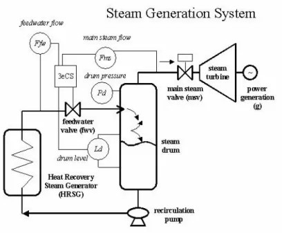
Our domain of interest lies on the steam generation system of a combined-cycle power plant. This system, which is aimed to provide superheated steam to a steam turbine, is basically composed by a recovery steam generator, a recirculation pump, control valves and interconnection pipes. A heat recovery steam generator (HRSG) is a process machinery capable of recovering residual energy from a gas turbine exhaust gases to generate high pressure (Pd) steam in a special tank (steam drum). The recirculation pump is a device that extracts residual water from the steam drum to keep a water supply in the HRSG (Ffw). The result of this process is a high-pressure steam flow (Fms) that keeps running a steam turbine to produce electric energy (g) in a power generator. The main control elements associated are the feed-water valve (fwv) and the main steam valve (msv). The complete process control domain is shown in figure 1.

During normal operation, a three-element feed–water control system (eCS) commands the feed-water control valve (fwv) to regulate the level (dl) and pressure (pd) in the drum. However, this traditional controller does not consider the possibility of failures in the control loop (valves, instrumentation, or any other process devices). Furthermore, it ignores whether the outcomes of executing a decision will help in the future to increase the steam drum lifetime, security, and productivity. So, the problem is to obtain a function that maps plant states to recommendations that considers all these aspects. Under the MDP framework, the potential failures are considered implicitly in a transition function, and the security and productivity goals are included in the reward. Thus, MDPs provide an adequate model for this problem; however, standard solutions explode computationally and can not deal with continuous variables. Next we give a brief review of MDPs, and then we present our method for solving continuous and complex MDPs, required for the power plan domain.

Fig. 1. A simplified diagram of steam generation process. Aimed to provide superheated steam to a turbine, the steam generation system is basically composed of a recovery steam generator, a recirculation pump, control valves and interconnection pipes

3 Factored Markov Decision Processes

A Markov decision process (MDP) [18] models a sequential decision problem, in which a system evolves in time and is controlled by an agent. The system dynamics is governed by a probabilistic transition function

Φ

that maps states

and actions to new states . At each time, an agent receives a reward

S

A

S

′

R

that depends on the current state

and the applied action

a

. Thus, they solve the problem of finding a recommendation strategy or policy that maximizes the expected reward over time and also deals with the uncertainty on the effects of an action.

s

Formally, an MDP is a tuple

M

=< , ,Φ, >

S A

R

, where

S

is a finite set of states

{s … s }

1

, ,

n .

A

is a finite set of actions for all states.

Φ : × ×

A S S

is the state transition function specified as a probability distribution. The probability of reaching state

s

′

by performing action

a

in state is written as

s

Φ , ,

(

a s s

′

)

. is the reward function.

R S

: × → ℜ

A

(

)

R s a

,

is the reward that the agent receives if it takes action

a

in state .

s

For the discrete discounted infinite-horizon case with any given discount factor

γ

, there is a policy

π

∗ that is optimal regardless of the starting state and that satisfies the Bellman equation [2]:

( )

_a

(

)

(

)

( )

s

V

π

s

max {R s a

γ

a s s V

π

s }

∈

′

′

=

, +

∑

Φ , ,

S (1)

In Continuous Markov Decision Processes (CMDPs) the optimal value function satisfies the Bellman fixed point equation:

( )

_a

[ (

)

(

) ( )

]

s

V s

max R s a

γ

a s s V s ds

′

′

′

′

=

, +

_∫

Φ , ,

(2)

Two methods for solving these equations and finding an optimal policy for an MDP are: (a) dynamic programming [18] and (b) linear programming.

In a factored MDP, the set of states is described via a set of random variables

X

=

{X … X }

₁

, ,

_n , where each i

X

takes on values in some finite domain

Dom X

(

_i

)

. A state defines a value

s

x

_i

∈

Dom X

(

_i

)

for each variable

X

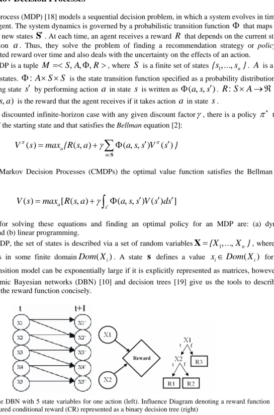
_i. The transition model can be exponentially large if it is explicitly represented as matrices, however, the frameworks of dynamic Bayesian networks (DBN) [10] and decision trees [19] give us the tools to describe the transition model and the reward function concisely.

Fig. 2. A simple DBN with 5 state variables for one action (left). Influence Diagram denoting a reward function (center). Structured conditional reward (CR) represented as a binary decision tree (right)

Let

X

_i denote a variable at the current time and

X

'

_i the variable at the next step. The of a DBN is a two–layer directed acyclic graph whose nodes are

transition graph

T

G

{

X … X

₁

, ,

_n

,

X

'

₁

, ,

… X

'

_n

}

, see figure 2 (left). Each node

X

'

_i is associated with a conditional probability distribution (CPD) , which is usually represented by a matrix (conditional probability table) or more compactly by a decision tree. The transition probability is then defined to be

(

' |

_i

(

' ))

_i

P X

_Φ

Parents X

(

a s s

i i

Φ , , ′

)

Π

_i

P x

_Φ

( ' |

_i

u

_i

)

where represents the values of the variables in . The next value X', often depends on a small subset of variables (Parents(X')) simplifying the transition function.

i

u

(

' )

_i

Parents X

The reward associated with a state often depends only on the values of certain features of the state. The relationship between rewards and state variables can be represented with value nodes in influence diagrams, as shown in figure 2 (center). The conditional reward tables (CRT) for such a node is a table that associates a reward with every combination of values for its parents in the graph. This table is locally exponential in the number of relevant variables. Although in the worst case the CRT will take exponential space to store the reward function, in many cases the reward function exhibits structure allowing it to be represented compactly using decision trees or graphs, as shown in figure 2 (right).

4 Qualitative MDPs

Although factored MDPs provide important reductions in the representation of transition and reward functions, in cases of problems with high dimensionality there can still be a large number of states involved. On the other hand, defining a suitable partition of the state space by a human expert is not an easy task. In this paper, we propose a novel approach to automatically define abstract states, and a procedure to approximate a decision model from data. In the proposed method, we gather information about the rewards and the dynamics of the system by exploring the environment. This information is used to build a decision tree [20] representing a small set of abstract states (called the qualitative partition) with equivalent rewards, and then is used to learn a probabilistic transition function using a Bayesian network learning algorithm [9]. The resulting approximate MDP model can be solved using traditional dynamic programming algorithms.

4.1. Qualitative states

A qualitative state1 (or q–state), , is a set of states (or a partition of the state space in the continuous case) that share similar immediate rewards. A qualitative state space, , is a set of q–states: , also called the qualitative partition.

i

q

Q

q q

1

, ,..

2

q

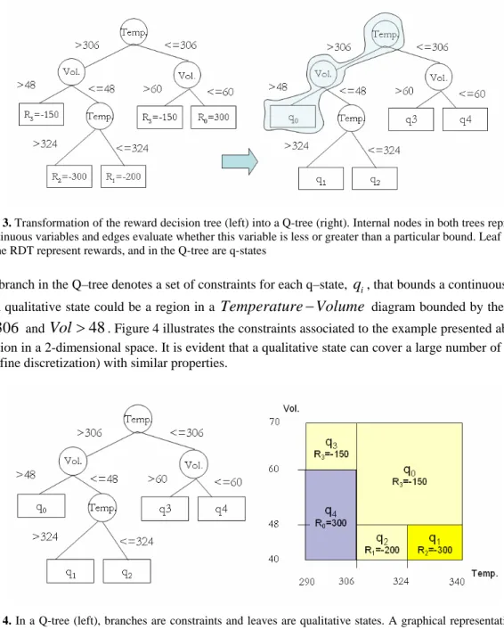
n

Similarly to the reward function in a factored MDP, the qualitative constrains that distinguish regions of the state space with different reward values, can be represented by a decision tree called Reward Decision Tree (RDT). Since a qualitative state maps directly a reward value, a qualitative partition can also be represented by a binary decision tree (Q–tree). In order to obtain a Q–tree, a reward decision tree (RDT) is first induced from simulated data and then transformed by simply renaming the reward values to q-state labels. Each leave in the Q–tree is labeled with a new qualitative state. Even for leaves with the same reward value, we assign a different qualitative state value. This produces more states but at the same time creates more guidance that helps to produce more adequate policies. Figure 3 illustrates this tree transformation for a simple two dimensional case that represents a Temperature-Volume diagram for an ideal gas.

Q

Fig. 3. Transformation of the reward decision tree (left) into a Q-tree (right). Internal nodes in both trees represent continuous variables and edges evaluate whether this variable is less or greater than a particular bound. Leaf nodes in the RDT represent rewards, and in the Q-tree are q-states

Each branch in the Q–tree denotes a set of constraints for each q–state, , that bounds a continuous region. For example, a qualitative state could be a region in a

Temperature

i

q

Volume

−

diagram bounded by the constraints: and . Figure 4 illustrates the constraints associated to the example presented above, and its representation in a 2-dimensional space. It is evident that a qualitative state can cover a large number of states (if we consider a fine discretization) with similar properties.

306

Temp

>

Vol

>

48

Fig. 4. In a Q-tree (left), branches are constraints and leaves are qualitative states. A graphical representation of the tree is also shown (right). Note that when an upper or lower variable bound is infinite, it must be understood as the upper or lower variable bound in the domain

4.2. Qualitative MDP Model Specification

We can define a qualitative MDP as an MDP with a qualitative state space. A hybrid (or qualitative–discrete) MDP is a factored MDP with a set of qualitative and discrete factors. In this case, we have a set of discrete variables, and the qualitative state space

Q

, which is an additional factor that concentrates all the continuous variables. Initially, only the continuous variables involved in the reward function are considered in the learning algorithm. Other continues variables are discretized arbitrarily; however, this initial discretization is improved in the refinement stage,

as described in Section 5. Thus, a hybrid qualitative-discrete state is described in a factored form as

{

X … X Q

1 n

}

=

, ,

,

h

s

, where

X … X

1

, ,

n are the discrete factors, and is a factor that represents the relevant continuous dimensions in the reward function.

Q

4.3. Learning Qualitative MDPs

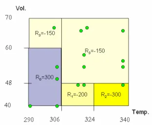
The Qualitative MDP model is learned from data based on a random exploration of the environment that allows recording state transitions, actions taken, and the associated reward values. To better understand how a training data set is recorded, consider the bi-dimensional domain described above, but now assuming that the system state can be modified by changing the temperature and volume values. The possible actions are increase/decrease the temperature, increase/decrease the volume, and do nothing (the null action). Figure 5 shows graphically a possible data trace produced by the random application of different actions on the system. Each dot in the figure represents a particular state (volume and temperature) that results after the application of a particular action. Each state is associated also to a reward value, which corresponds to the different regions in figure 5. Thus, after exploring the environment we obtain a data set that records for each action, sequentially from

t

=

1

to , the action, resulting state and reward. So for the gas example, each data record will contain: =(Temperature, Volume, Action, Reward). From this data set, a decision model is obtained, and then solved using the value iteration algorithm.

N

i

Data

Formally, this idea can be described as follows. Given a set of state transitions represented as a set of random variables,

{

1

}

j

O

=

X A X

_t

, ,

_t+ , for

j

= , ,...,

1 2

N

, for each state and action

A

executed by an agent, and a reward (or cost)

R

j associated to each transition, we learn a qualitative factored MDP model:

1. From a set of simulated transitions

{

O R

,

}

induce a reward decision tree,

RDT

, that predicts the reward function

R

in terms of continuous and discrete state variables,

X … X Q

₁

, ,

_k

,

. For the gas example, this tree corresponds to the one shown in Figure 3, left.

2. Obtain from the decision tree (

RDT

) the set of constraints for the continuous variables relevant to determine the qualitative states (q–states) in the form of a Q-tree. In terms of the domain variables, we obtain a new variable

Q

representing the reward-based qualitative state space whose values are the q–states. This transformation is illustrated in Figure 3 for the ideal gas example, with the resulting Q-tree (right). This Q-Tree is shown again in Figure 4 (left), which also shows the qualitative partition obtained (right), where the state space is divided into 5 qualitative states,

q q …q

₀

, ,

_{1 4}.

3. Qualify data from the original sample in such a way that the new set of attributes is the variable, the remaining discrete and continuous variables not included in the decision tree, and the action

Q

A

. The continuous variables not considered in the RDT tree are discretized in a coarse way with equal size intervals (this initial discretization is improved in the refinement stage). This transformed data set is called the qualified data set. For the example, the state in each record in the data set will be represented by the corresponding qualitative state, , instead of the numeric values of the original state variables, Vol. and Temp. These q–states are determined in terms of the partition of the state space, as shown in Figure 4.

0

q …q

₄

4. Format the qualified data set in such a way that the attributes follow a temporal causal ordering. For example variable

Q

_t must be set before

Q

_t+1,

X

1_t before

X

1_t+1, and so on. The whole set of attributes

should be the variable

Q

in time , the remaining system variables,

t

X … X

₁

, ,

_k, in time

t

, the variable

Q

in time

t

+

1

, the remaining system variables in time

t

+

1

, and the action

A

. Thus, for the gas example, each record in the qualified data set will be:

(

q a r

_i

, ,

_{i i t}

)

, where is the q–state, is the action, is the reward, and

t

is time, from to

t

N

( is the number of steps in the exploration).

i

q

a

_i

r

_i

0

5. Prepare data for the induction of a 2-stage dynamic Bayesian net. According to the action space dimension, split the qualified data set into

| |

A

sets of samples, one for each action. In the gas case there will be 5 sets, one for each possible action: increase/decrease the temperature, increase/decrease the volume, and do nothing.

6. Induce the transition model for each action,

A

_j, using a Bayesian network learning algorithm [9]. So for our running example, we will induce a DBN to represent the transition model for each of the 5 actions, all in terms of the q–state variables.

Fig. 5. Exploration trace for the ideal gas domain. Each dot in the figure represents a data point in the exploration, with its corresponding state (Vol. and Temp.), reward (determined by the region), and action applied to reach this state. Thus, by applying random actions on the system, it is possible to capture the effects of these actions (new states) and the immediate reward received per state

At the end of this process we have learned a qualitative MDP model of the problem based on a random exploration of the environment, and the qualitative partition obtained from the reward decision tree. In this model, the transition function is represented as a set of 2–stage DBNs, one per action, and the reward by a decision tree; both in terms of the q–state variables. As mentioned before, if there are additional variables that are not part of the reward function, these are just incorporated into the model.

This initial model represents a high-level abstraction of the continuous state space and can be solved efficiently using a standard technique, such as value iteration, to obtain the optimal policy. For instance, in the ideal gas example, the resulting policy will give the optimal action for each q-state,

q …q

_{0 4}.

This approach has been successfully applied in several domains; however, in some cases the initial abstraction can miss some relevant details of the domain and consequently produce sub-optimal policies. We improve this initial partition through a refinement stage described in the next section.

5 Qualitative State Refinement

We have designed a value-based algorithm that recursively selects and partitions abstract states with high utility variance. If there are continuous dimensions that were not included in the initial Q-tree (because they do not affect the reward), these are incorporated at this stage. For this, we simply extend the Q-tree with the additional dimensions with an initial, coarse discretization. Before we see in detail the refinement algorithm, we need to define some relevant concepts.

The border of state,

s

_i, is defined as the set of states,

S

_j

= , ,

{

s … s

_{1 n}

}

, such that is a neighbor of ; that is, they are adjacent in at least one dimension. A region is defined as

k

s

∈

S

j j i

s

i i

r

= ∪

s

S

, that is, a state and its border states. For instance, in the ideal gas example,

q

₀ and

q

₄ are the border states of

q

₃, and

r

₃

= , ,

{

q q q

_{3 0 4}

}

, see figure 4.

The utility variance of a region, , that corresponds to state

r

_i

s

_i, is defined as:

2 2 1

1

(

)

i n n r qk k

S

V

n

=

=

∑

−

V

_r (3)

where

n

is the number of border states for , is the value of each state, , in the region, and is the average value of the states in the region. The value for each state is obtained when we solve the qualitative MDP, as described in the previous section.

i

s

V

_qk

s

_k

V

_rn

The utility gradient gives the difference in utility between one state, , and one of its border states, , and it is defined as follows: i

s

s

_k

|

|

i

V

i

V

k

δ

=

−

(4)

The hyper-volume of a state, , corresponds to the space occupied by the state and its obtained by the product of its dimensions: i

s

d

1 d i l l

hv

x

=

=

∏

(5) where

x

_l is the value for each dimension

l

.

The refinement algorithm has as input the initial qualitative partition obtained in the learning stage and an initial solution for this qualitative MDP. It also requires a minimum hyper-volume for a state defined by the user, as this depends on the application. It proceeds as follows:

1. Initialize all the states as unmarked.

2. While there is an unmarked qualitative state greater than the minimum hyper-volume: (a) Save a copy of the previous MDP (before the partition) and its solution. (b) Obtain the utility variance for each state in its corresponding region.

(c) Select a qualitative state with the highest variance in its utility value with respect to its neighbors, name it

q

_i.

(d) For the qualitative state

q

_i select a continuous dimension to split it, from (

x x … x

₀

, , ,

_{1 n}), such that it has the highest utility gradient with respect to its border states along this dimension.

(e) Bisect the q-state

q

_i over the selected dimension (divide the state in two). (f) Solve the new MDP, which includes the new partition, using value iteration.

(g) If the new MDP has the same policy as before, mark the original state before the partition, and return to the previous MDP, otherwise, accept the refinement and continue.

i

q

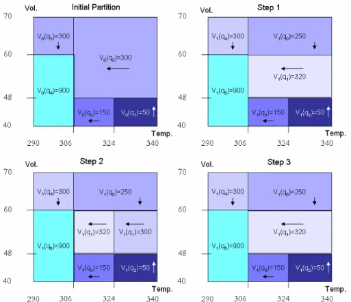
The refinement process is now described for the ideal gas example. Figure 6 illustrates 3 steps in the abstraction process for the example in figure 4. The initial partition is shown at the top–left. Let us assume that the state has the highest variance in utility with respect to its neighbors,

0

q

1 2 3 4

q q q q

, , ,

; and that

Vol

is the dimension with the highest difference in utility. A bisection is then inserted to split state in the new states and (Step 1, top– right). The remaining states are relabeled to preserve a progressive numbering. After solving the new MDP and verifying that the policy has changed, the bisection is accepted and the algorithm proceeds to Step 2 (bottom-left). In this case is the state with the highest variance and it is split on the

Te

.

0

q

q

₀

q

₁

1

q

mp

.

dimension which is the dimension

with the highest difference in utility. However, after solving the new MDP, the policy does not change, so the division is canceled and it returns to the previous partition, as depicted in the bottom-right of figure 6. Thus, this state will be marked and not considered for subsequent partitions.

Fig. 6. An example of the qualitative refinement process for a two-dimension state space. Initial partition: the initial solution obtained before, for each q–state its value and optimal action are shown. Step 1: the state with highest variance is bisected along the dimension with highest variance, Vol. Note that the q–states have been renamed. Step 2: now is partitioned along the Temp. dimension. Step 3: as there is no change in policy for the partition in Step 2, it returns to the partition in Step 1

0

q

1

q

6 AsistO: A Recommender System for Power Plants

AsistO is an intelligent assistant that provides useful recommendations for training and on-line assistance in the power plant domain. AsistO was built specially to demonstrate the potential of the qualitative MDP approach to solve planning problems in complex domains. The recommender system is coupled to a power plant simulator capable to partially reproduce the operation of a combined cycle power plant (CCPP), in particular, the steam generation process (HRSG), described in section 2.

The simulator (figure 7) is provided with controls for setting up the power conditions in the gas and steam turbines (nominal load, medium load, minimum load, hot standby condition, low speed, and start-up). It includes an operation panel to configure load demands, unit trips, shutdowns, and other high level operations in different plant subsystems. It also includes a visualization tool for tracking the behavior in time of a set of variables selected by the user, and a function for recording historical data.

Fig. 7. A screen shot of human–computer interface of the steam generation simulator. The simulator provides controls, an operation panel, and data visualization tools

6.1. General Architecture

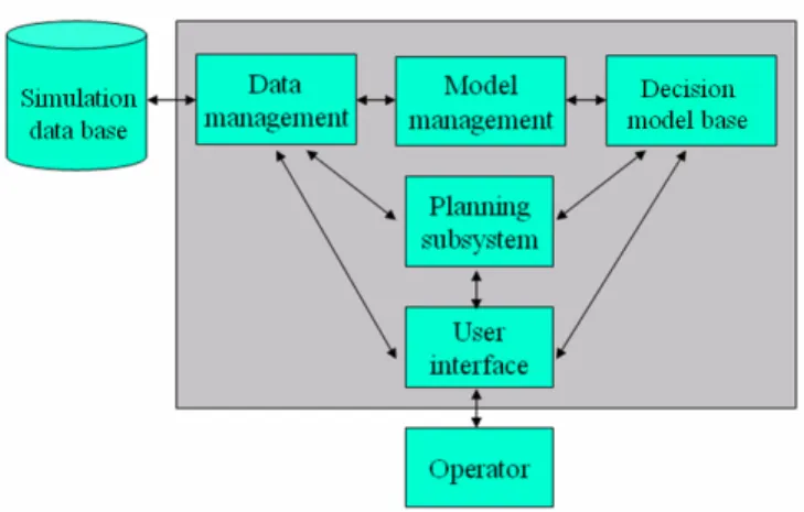
The AsistO recommender system is composed by a decision model base, a simulation data base, and the following subsystems: i) data management, ii) model management, iii) planning subsystem, and iv) user interface. Figure 8 shows AsistO’s general architecture.

The simulation data base allocates the process signals generated by the simulator (outputs), and the control signals (inputs) sent by an instructor to set up a specific electric load or failure condition in the process. On the other hand, the decision model base stores the qualitative MDP model of the process and its solution in form of a policy. That is, it has the optimal action that will be recommended to the operator for every state of the plant subprocess considered. The policy is based on a factored representation of the plant q-states (see section 4.2), and represented in the form of algebraic decision diagrams (ADDs) [14].

Fig. 8. AsistO’s general architecture. Given a state of the plant obtained from the simulation data base, the planning subsystem queries a recommendation to the decision model base. This recommendation is presented to the operator via the user interface

The data management subsystem is composed by a set of tools for data administration and analysis. The model management subsystem manipulates the transition and reward models, and the utility and policy functions stored in the decision model base. The transition model management system was implemented in Elvira [8] (which also was adapted to compute Dynamic Bayesian Networks), and the reward model management system using Weka [22]. The management of the policy and utility models is carried out using SPUDD [14], which includes model query and printing capabilities.

The planning subsystem in AsistO is also based on SPUDD [14], which implements a very efficient version of the value iteration algorithm for MDPs as inference method. The planning subsystem first approximates the decision models using the data allocated in the simulation data base. Transition and reward models are respectively learned using the K2 [9] algorithm available in Elvira, and the C4.5 algorithm available in Weka (J4.8) [20]. Then it uses these models and its inference algorithms to obtain an optimal policy, from which the recommendations that will be given to the operator are obtained. The resulting transition and reward functions, and policy and utility functions are then stored in the decision model base. The planning subsystem transforms the continuous plant state into the qualitative representation described in sections 4 and 5 for problem specification and policy query purposes.

The user interface provides the communication with the environment. In this case, the power plant simulator is the environment, and the operator is the actor that executes the recommendations that modify the environment. The user interface provides controls for command execution, load selection, failure simulation, and recommendation display. This module, which can also be used as a supervision console, includes the controls for random exploration and system sampling for the learning purposes described in section 4.3. It also provides a graphical interface to observe how fast the correct execution of recommendations impact on the plant operation. The main screen of the user interface is shown in Figure 9.

Currently AsistO is used for operator training. In a training session, the planning subsystem obtains the plant q-state from the simulation data base. Then it queries the policy function for the current q-q-state in the model base to obtain a recommendation. Both, current q-state and recommendation are shown graphically to the operator through the user interface, who finally decides whether or not to execute the recommended command. The sequential execution of these recommendations will help the operator to get the plant to an optimal operating condition.

Fig. 9. User Interface. It is the graphical link between the recommender system and the operator. It includes supervision features, problem specification utilities, display console, and manual control capabilities

6.2. Experimental Results

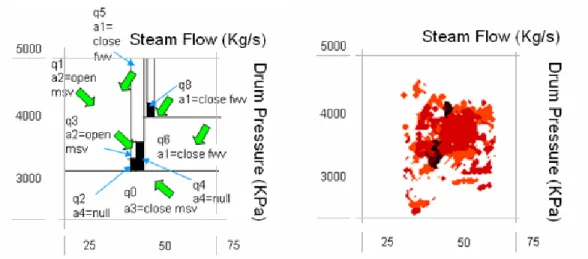
We used AsistO to run two sets of experiments with different complexities. In the first set of experiments, we specified a 5-action hybrid problem with 5 variables (

Fms Ffw Pd g d

,

,

, ,

). We also defined a simple binary reward function based on the safety parameters of the drum ( and ). The relationship between their values and the reward received can be seen in figure 10 (left). Central black squares denote safe states (desired operation regions), and white zones represent non-rewarded zones (indifferent regions). To learn the model and the initial abstraction, samples of the system dynamics were gathered using simulation. Black dots in figure 10 (right) represent sampled states with positive reward, red (gray) dots have no reward, and white zones were simply not explored. Figure 10 (left) shows the state partition and policy found (arrows) by the learning system. For this simple example, although the resulting policy is not very detailed ( are quite large), it directs the plant to the optimal operating condition (black region in the middle). When analyzed by an expert operator, this control strategy is near-optimal in most of the abstract states.

Pd

Fms

qstates

We solved the same problem but adding two extra variables, the position for valves

msv

and

fwv

, and using 9 actions (all the combinations of open-close valves

msv

and

fwv

). We also redefined the reward function to maximize power generation, , under safe conditions in the drum. Although the problem increased significantly in complexity, the policy obtained is “smoother” than the 5-action simple version presented above. To give an idea about the computational saving, for a fine discretization (15,200 discrete states) this problem was solved in 859.2350 seconds, while our abstract representation (40 q-states) took only 14.2970 seconds. In both cases, the solutions were found using the SPUDD system [14].

g

In summary, the first experiment shows that the proposed approach obtains approximately optimal policies; while the second experiment demonstrates a significant reduction in the solution time in comparison to a fine discretization of the state space.

Fig. 10. Process control problem. Left: qualitative state partition in terms of the Steam Flow and Drum Pressure. For each q–state it shows the optimal action (arrows). The black region represents the desired operating state (high reward). Right: an image of the exploration trace, where black dots represent sampled states with positive reward, red dots (gray) are sampled states with no reward, and white regions are unexplored zones

7 Conclusions and Future Work

In this paper, we presented a novel and practical model-based learning approach with iterative refinement for solving continuous and hybrid Markov decision processes. In the first phase we use an exploration strategy of the environment and a machine learning approach to induce an initial state abstraction. We then follow a refinement process to improve the initial abstraction by performing local tests on the variance of utility values. Our approach creates significant reductions in space and time allowing to solve efficiently continuous and hybrid problems. We tested our method in a power plant domain using AsistO, showing that this approach can be applied to complex domains where a simple dicretization approach is not feasible or computationally too expensive.

Since AsistO is aimed either for operation assistance and operator training, we are currently developing an extra module that explains the recommended commands generated by the planning subsystem and, provides, after a bad decision, the reason why a recommendation should have been followed. We plan to extend the planning subsystem to support partially observable MDPs, and use the AsistO architecture in other power plant applications.

As future research work we will like to improve our refinement strategy to select a better segmentation of the abstract states and consider alternative search strategies. We also plan to test our approach in other domains.

Acknowledgments

This work was supported jointly by the Instituto de Investigaciones Eléctricas, Mexico and CONACYT Project No. 47968.

References

1. J. Baum and A. E. Nicholson.Dynamic non-uniform abstractions for approximate planning in large structured stochastic domains. In PRICAI’98 – Proceedings of the 5th Pacific Rim International Conference on Artificial Intelligence, pages 587–598, Singapore, 1998.

2. R.E. Bellman. Dynamic Programming. Princeton U. Press, Princeton, N.J., 1957.

4. D. P. Bertsekas and J.N. Tsitsiklis. Neuro-dynamic programming. Athena Sciences, 1996.

5. B. Bonet and J. Pearl. Qualitative MDPs and POMDPs: An order-of-magnitude approach. In Proceedings of the 18th Conf. on Uncertainty in AI, UAI-02, pages 61–68, Edmonton, Canada, 2002.

6. C. Boutilier, T. Dean, and S. Hanks. Decision-theoretic planning: structural assumptions and computational leverage. Journal of AI Research, 11:1–94, 1999.

7. C. Boutilier, M. Goldszmidt, and B. Sabata. Continuous value function approximation for sequential bidding policies. In Kathryn Laskey and Henri Prade, editors, Proceedings of the 15th Conference on Uncertainty in Artificial Intelligence (UAI-99), pages 81–90. Morgan Kaufmann Publishers, San Francisco, California, USA, 1999.

8. Elvira Consortium. Elvira: an environment for creating and using probabilistic graphical models. Technical report, U. de Granada, Spain, 2002.

9. G. F. Cooper and E. Herskovits. A bayesian method for the induction of probabilistic networks from data. Machine Learning, 1992.

10. T. Dean and K. Kanazawa. A model for reasoning about persistence and causation. Computational Intelligence, 5:142–150, 1989.

11. Z. Feng, R. Dearden, N. Meuleau, and R. Washington. Dynamic programming for structured continuous Markov decision problems. In Proc. of the 20th Conf. on Uncertainty in AI (UAI-2004). Banff, Canada, 2004. 12. C. Guestrin, M. Hauskrecht, and B. Kveton. Solving factored MDPs with continuous and discrete variables.

In Twentieth Conference on Uncertainty in Artificial Intelligence (UAI 2004), Banff, Canada, 2004.

13. M. Hauskrecht and B. Kveton. Linear program approximation for factored continuous-state Markov decision processes. In In Advances in Neural Information Processing Systems NIPS(03), pages 895– 902, 2003.

14. J. Hoey, R. St-Aubin, A. Hu, and C. Boutilier. SPUDD: Stochastic planning using decision diagrams. In Proc. of the 15th Conf. on Uncertainty in AI, UAI-99, pages 279–288, 1999.

15. L. Li and M. L. Littman. Lazy approximation for solving continuous finite-horizon MDPs. In AAAI-05, pages 1175–1180, Pittsburgh, PA, 2005.

16. R. Munos and A. Moore. Variable resolution discretization for high-accuracy solutions of optimal control problems. In Thomas Dean, editor, Proceedings of the 16th International Joint Conference on Artificial Intelligence (IJCAI-99), pages 1348–1355. Morgan Kaufmann Publishers, San Francisco, California, USA, August 1999.

17. J. Pineau, G. Gordon, and S. Thrun. Policy-contingent abstraction for robust control. In Proc. of the 19th Conf. on Uncertainty in AI, UAI-03, pages 477–484, 2003.

18. M. L. Puterman. Markov Decision Processes. Wiley, New York, 1994.

19. J.R. Quinlan. Induction of decision trees. Machine Learning, 1(1):81–106, 1986.

20. J.R. Quinlan. C4.5: Programs for machine learning. Morgan Kaufmann, San Francisco, Calif., USA., 1993. 21. R. S. Sutton and A.G. Barto. Reinforcement Learning: An Introduction. MIT Press, 1998.

22. I.H. Witten. Data Mining: Practical Machine Learning Tools and Techniques with Java Implementations, 2nd Ed. Morgan Kaufmann, USA, 2005.

Alberto Reyes is a researcher at the Electrical Research Institute in México (IIE) and part-time professor at Instituto

Tecnológico y de Estudios Superiores de Monterrey (ITESM) campus México City. His research interests include decision-theoretic planning, machine learning, and their applications in robotics and intelligent assistants for industry. He received a PhD in Computer Science from ITESM campus Cuernavaca.

L. Enrique Sucar is a Senior Researcher at the National Institute for Astrophysics, Optics and Electronics (INAOE)

in Puebla, Mexico. His research interests include reasoning under uncertainty in artificial intelligence, mobile robotics and computer vision. He received a B.S. in Electronics and Communications Engineering from the Monterrey Institute of Technology, in Monterrey, Mexico, a M.Sc. in Electrical Engineering from Stanford University, and a Ph.D. degree in Computer Science from Imperial College, London. He has been president of the Mexican AI Society, member of the Advisory Committee for IJCAI, and member of the National Research System and the Mexican Academy of Science.

Eduardo F. Morales is a Senior Researcher at the National Institute for Astrophysics, Optics and Electronics

(INAOE) in Puebla, Mexico. His research interests include machine learning and mobile robotics. He received a B.Sc. degree in Physics Engineering from Univeridad Autonoma Metropolitana, in Mexico City, an M.Sc. in Artificial Intelligence from Edinburgh University, Scotland, and a Ph.D. degree in Computer Science from The Turing Institute- Strathclyde University, in Glasgow. He is a member of the National Research System in Mexico.