Econometric Tools for Detection of Collusion Equilibrium in the Industry

Full text

(1)DYNAMIC ECONOMETRIC MODELS. gH. ou. se. Vol. 9 – Nicolaus Copernicus University – Toruń – 2009. Sylwester Bejger. ic. Pu b. lis. hin. Nicholas Copernicus University in Toruń. sit y. Sc. ien. tif. Econometric Tools for Detection of Collusion Equilibrium in the Industry. op er n. icu sU. niv er. A b s t r a c t. The article presents the notion of detection of overt or tacit collusion equilibrium in the context of choice of the appropriate econometric method, which is determined by the amount of information that the observer possesses. There has been shown one of the collusion markers coherent with an equilibrium of the proper model of strategic interaction – the presence of structural disturbances in the price process variance for phases of collusion and competition. The Markov Switching Model with switching of variance regimes has been proposed as a proper theoretical method detecting that type of changes without prior knowledge of switching moments. In order to verify the effectiveness of the method it has been applied to a series of lysine market prices throughout and after termination of its manufacturers’ collusion.. ico lau. sC. K e y w o r d s: explicit and tacit collusion, collusive equilibrium, cartel detection, lysine, price variance, Markov switching model. eN. 1. Introduction. ©. Co py. rig. ht. by. Th. The equilibrium of players’ collusion in the industry may occur as a consequence of players’ strategic interaction of the overt or tacit collusion nature. Although these two types of interaction are described by means of different models of game theory with various informative assumptions, their equilibriums are characterized by similar consequences for the industry, i.e.: a) the occurrence players’ market power leading to the loss of social wealth (above-normal PCM), b) the limitation of competition and the impediment of the industry development . The article presents one of collusion markers resulting from the theoretical model of tacit collusion, which is price rigidity in the collusion phase, and proposes the application of the Markov Switching Model of MS-AR-GARCH type in order to detect structural changes in market price variance, and thereby to.

(2) Sylwester Bejger. 28. se. verify the presence of the aforementioned marker. The preliminary verification of usefulness of the proposed econometric method constitutes a research problem. For this purpose, in the empirical section there has been applied the proposed model for a series of market prices of cartel players – lysine manufacturers.. gH. ou. 2. Collusion and Its Quantitative Detection. ©. Co py. rig. ht. by. Th. eN. ico lau. sC. op er n. icu sU. niv er. sit y. Sc. ien. tif. ic. Pu b. lis. hin. Collusion constitutes a serious problem in the market economy. If we take into account only overt collusion (mainly in the area of English-speaking reporting) between 1990 – 2005, 283 cartels were confirmed (so called hard core cartels) with national and global scope of operation, however, it has been estimated that as little as 30% of overt collusion are detected and punished. There are no data concerning tacit collusion. The above mentioned 283 cartels influenced sales of 2.1 trillion USD, caused unjustifiable price overcharge of the value of 500 bn USD and were punished with pecuniary penalty of the nominal value amounting to 25.4 bn USD (Connor, Helmers, 2006). Taking into account the fact how common and harmful such collusion is, it seems natural that it should be quickly detected. Unfortunately, although theoretical models of overt or tacit collusion are described very well as research hypotheses concerning players’ behavior, their empirical verification presents great difficulties. It happens mainly due to the fact that the players participating in collusion have an advantageous position over the observer in the form of private information. Moreover, the resources of public statistics are frequently very humble on the disaggregation level of the industry or individual players. Thus, it is not difficult to ascertain that econometric methods, that are, on the one hand, economical as far as the use of statistical data is concerned, and, on the other hand, coherent with the model hypothesis, are particularly valuable. Currently known econometric methods of detection can be divided into direct and indirect methods: a) direct - the assessment of strategy profile in equilibrium that is consistent with the assumed collusion model, verification of the hypothesis on conformity with theoretical equilibrium, b) indirect - measurement and/or identification of market power or detection of so called collusion markers (non-competitive behaviors), i.e, certain, characteristic for collusion, disorders concerning: − the relation between players’ prices and market demand changes, − price and market share stability, − the relation between players’ prices, − investment in production capacity..

(3) Econometric Tools for Detection of Collusion Equilibrium in the Industry. 29. ien. tif. ic. Pu b. lis. hin. gH. ou. se. When it comes to statistical data, group a) methods are very demanding, their applications are very rare and they are possible only in specific circumstances1. Group b) methods are much more common. The following basic methods are enumerated in the order of intensity of the use of statistical data: − the study of structural changes in price volatility , − non-parametric method based on revealed preferences, − the Osborne – Pitchik test, − the study of asymmetry of price reactions, − Hall’s method, − the assessment of residual demand elasticity, − the Panzar – Rosse method, − CPM method.. Sc. 3. Price Disorders Characteristic for Collusion. ©. Co py. rig. ht. by. Th. eN. ico lau. sC. op er n. icu sU. niv er. sit y. One of the most promising collusion markers are markers that are based on the analysis of changes in price processes and/or market shares. In accordance with known tacit collusion models: 1. the player’s (players’) price and supply are negatively correlated, the price is ahead of the demand cycle, the stochastic process of market price undergoes changes of the regime type (Green, Porter, 1984; Rotemberg, Saloner, 1986; Haltiwanger, Harrington, 1991), 2. the price process variance is on average lower for collusion phases and may undergo changes of the regime type (Athey, Bagwell, Sanchirico, 2004; Connor, 2004; Abrantes-Metz, Froeb, Geweke, Taylor, 2006; Bolotova, Connor, Miller, 2008), The application marker 2 is particularly promising in practice. It is justified by the fact that the requirements for this marker concerning data are very little (market price is sufficient) and it has clear theoretical justification. Lower price volatility in the collusion phase results directly from the equilibrium properties of SPPE type (symmetric perfect public equilibrium) of the price super-game with standard assumption concerning sufficiently high discount rate. For the strategy profile in the equilibrium of this game, players: − achieve higher payments than in competitive equilibrium (cartel payments), − in the collusion phase, players’ prices are insensitive to costs shocks (players avoid price changes, even at the cost of effectiveness, not to cause switching to penalty phase).. 1. For example, see Slade (1992)..

(4) Sylwester Bejger. 30. It should be noted that the necessity of using a number of observations including both competition and collusion phases and high product homogeneity of the analyzed trade is one of the marker’s drawbacks.. se. 4. Econometric Method Verifying Marker’s Presence. ©. Co py. rig. ht. by. Th. eN. ico lau. sC. op er n. icu sU. niv er. sit y. Sc. ien. tif. ic. Pu b. lis. hin. gH. ou. The works conducted so far that are connected with collusion detection on the basis of the detection of structural changes in variance included the application of the descriptive statistics methods for the comparison of variance level in collusion and competition phases (Abrantes-Metz, Froeb, Geweke, Taylor, 2006) and the application of ARCH / GARCH specification for the market price process together with additional 0-1 variable describing collusion and competition phases (Bolotova, Connor, Miller, 2008, further BCM ). This paper suggests using the Markov Switching Model of MS(M)(AR(p))GARCH(p,q) type as an econometric method verifying the marker for the variance and/or the average (constant) of the price process 2. The application of this model has the following advantages: − it is theoretically coherent with the structure of equilibrium strategy of the super-game model, − it allows to model structural changes of process variance directly, without the use of additional artificial variables; such modeling is not possible in, e.g. ARCH / GARCH specification, − it is coherent with informative asymmetry between cartel members and the observer. MS(AR)GARCH specification does not require observation (knowledge) of the state variable, thus it may be used for actual detection of variance regimes and objective determination of switching moments, that is the detection of collusion and competition phases. The form of the general MS(M)(AR(p))GARCH(p,q) model is a development version of a wellknown MS model (Hamilton, 1989; Hamilton, Susmel, 1994; Krolzig, 1998; Stawicki, 2004; Davidson, 2004). The application of the model with regimes in variance refers mainly to high frequency data, such as currency rates, rates of return from financial instruments, prices of electric energy3. The general form of switching model which has been applied can be written down as4:. 2 According to Krolzig this type of model could be described as MSI(M)H-AR(q) with GARCH(p,q) component, Krolzig (1998). 3 For example, refer to Fong (1998), Włodarczyk, Zawada (2005, 2007), Kośko, Pietrzak (2007). 4 There are various forms of notation, this one is from Davidson (2004)..

(5) Econometric Tools for Detection of Collusion Equilibrium in the Industry. 31. p. y t = α 0 St + ∑ φ mSt y t − m + u t ,. (1). m =1. where: ut = ht1/ 2 et oraz et ~ i.i.d .(0,1),. se. ∞. ou. ht = β 0 St + ∑ β mSt u t2−m ,. (2). gH. m =1. tif. ic. Pu b. lis. hin. The conditional variance equation (2) uses ARCH(∞) specification which also includes models of GARCH (p,q) class. In model (1),(2) each parameter may be potentially a random variable switched between the values from a finite set of values depending on the actual state of S t where S t = 1, ..., M .. sit y. Sc. { }. with fixed transition probabilities pij where:. ien. Variable S t is assumed to be the exogenous, homogeneous Markov process. niv er. pij = Pr( S t = j S t −1 = i ) .. f ( yt | S t = j , Ω t −1 ) Pr(S t = j | Ω t −1 ). ∑i =1 f ( yt | S t = i, Ω t −1 ) Pr(S t = i | Ω t −1 ) M. ,. (3). op er n. Pr( S t = j | Ω t ) =. icu sU. The probability that the observed process y t is in the state j in the period t is presented by means of the filtering (updating) equation:. sC. where Ω t signifies the entire information available at moment t, and: Pr( S t = j | Ω t −1 ) = ∑i =1 p ij Pr(S t −1 = i | Ω t −1 ),. ico lau. M. (4). eN. where transition probability pij constitutes M(M-1) parameters to be estimated.. Th. The form of conditional density function of observed variable:. by. f (. | S t = j , Ω t −1 ),. Co py. rig. ht. requires making an assumption concerning the type of distribution. Estimation of model parameters may be obtained through maximum likelihood method. For this purpose a likelihood function is used: T. ©. L = ∑ log Pr ∑i =1 f ( yt | St = j , Ω t −1 ) Pr(St = j | Ωt −1 ), M. (5). t =1. The maximization of function (5) is conducted by means of a very well known method, Expectation Maximization (EM) algorithm (Krolzig, 1998, p. 8)..

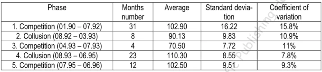
(6) Sylwester Bejger. 32. 5. Empirical Verification. se. The collusion of lysine producers5 was proved in 1996. The test includes monthly average lysine prices on the USA market in the period between 01/90 – 06/966. Within this period, on the basis of collected evidence (Connor, 2001) the following phases may be distinguished (Table 1). Coefficient of variation 15.8% 10.9% 11% 7.8% 9.3%. gH. Standard deviation 16.22 9.83 7.72 8.55 9.51. hin. Average. Pu b. lis. 102.90 90.13 70.50 110.30 102.50. tif. 1. Competition (01.90 – 07.92) 2. Collusion (08.92 – 03.93) 3. Competition (04.93 – 07.93) 4. Collusion (08.93 – 06.95) 5. Competition (07.95 – 06.96). Months number 31 8 4 23 12. ic. Phase. ou. Table 1. The statistics of lysine price (prices per pound). icu sU. niv er. sit y. Sc. ien. The purpose of the empirical research is to check to what degree the model with the proposed specification may be used to detect changes of the regime type in the variance of the process generating data, and thereby detect collusion phases. Such verification is possible due to the knowledge of the collusion history, provided that this case has been correctly determined (i.e., no significant evidence was omitted during the trial). Initially, there was verified a hypothesis on variances equality for two comparable phases. Table 2 summarizes this step.. Test F. ico lau. Brown-Forsythe. sC. Bartlett. op er n. Table 2. The value of statistics for the variance equality test in phase 1 and 4 7.6064. (0.005). 3.9206. (0.053). 3.2106. (0.003). Note: p-values given in brackets.. ©. Co py. rig. ht. by. Th. eN. On the basis of the test it can be ascertained that variances in both phases are significantly different. Next, the properties of the examined series were checked in terms of the distribution characteristics and autocorrelation, stationarity and homoscedasticity of residuals. The results of this part of research are included in Table 3.. 5. Lysine is an basic amino acid required as a feed component in hog, poultry and fish produc-. tion. 6. The prices are from Connor, (2000), appendix A, Table A2..

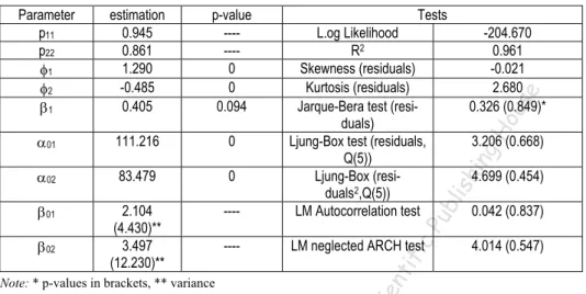
(7) Econometric Tools for Detection of Collusion Equilibrium in the Industry. 33. Table 3. Characteristics of series ADF test. Jarque-Bera 7.634 (0.021) normality test 3.081 Ljung – Box test 145.260 (0.000) for levels – Q(5) LM test for heteroscedasticity of residuals. -0.765. Kurtosis. -3.627* (0.007) 0.160**. KPSS test. 9.685 (0.002). se. Skewness. gH. ou. Note: p- values given in brackets, * value of t statistics (critical values for 1%, 5%, 10% sig. levels – (-3.519), (-2.900), (-2.587), ** value of LM statistics (asympt. critical values for 1%, 5%, 10% sig. levels – 0.739, 0.463, 0.347).. niv er. sit y. Sc. ien. tif. ic. Pu b. lis. hin. The series is skewed, the hypothesis of normal distribution was rejected and by means of test with different configuration of hypotheses the series stationarity was confirmed. After removing autocorrelation, there is explicit heteroscedasticity of a random component, which indicates relations in the variance which were not included in the model. In the next stage of the research a number of models of MS(k)(AR(p))GARCH(p,q) type was constructed and estimated with the use of maximum likelihood method. The best results, when it comes to the model properties, were achieved for MS(2)(AR(2))GARCH(1;0) specification in the form of:. where: u t = ht1 / 2 et oraz. op er n. m =1. icu sU. 2. y t = α 0 St + ∑ φ m y t − m + u t ,. (6). et ~ i.i.d .(0,1),. ico lau. S t = 1;2.. sC. ht = β 0 St + β1ut2−1 ,. (7). ©. Co py. rig. ht. by. Th. eN. This specification assumes controlling the observable price process through non-observable stochastic process of state variable st, which is assumed to be a homogeneous Markov chain of two states and proper matrix of transition probabilities between states. A constant and unconditional error variance are parameter which depends on the regime. Moreover, regardless of the regime, the average of a series is described by AR(2) process, whereas, GARCH(1;0) component is present in the variance. Table 4 shows estimation results..

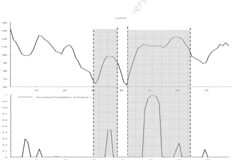
(8) Sylwester Bejger. 34. Table 4. Estimation results MS(2)(AR(2))GARCH(1;0). 0. α02. 83.479. 0. β01. 2.104 (4.430)** 3.497 (12.230)**. -------. LM neglected ARCH test. 3.206 (0.668). 4.699 (0.454). Pu b. ic. 0.042 (0.837) 4.014 (0.547). tif. β02. se. 111.216. -204.670 0.961 -0.021 2.680 0.326 (0.849)*. ou. α01. Tests L.og Likelihood R2 Skewness (residuals) Kurtosis (residuals) Jarque-Bera test (residuals) Ljung-Box test (residuals, Q(5)) Ljung-Box (residuals2,Q(5)) LM Autocorrelation test. gH. p-value ------0 0 0.094. hin. estimation 0.945 0.861 1.290 -0.485 0.405. lis. Parameter p11 p22 φ1 φ2 β1. Sc. ien. Note: * p-values in brackets, ** variance. ©. Co py. rig. ht. by. Th. eN. ico lau. sC. op er n. icu sU. niv er. sit y. The most essential question is whether the proposed model may serve the assumed objective, i.e. collusion detection. It can be estimated on the basis of precision of regime detection. Figure 1 shows the values of the observed variable and smoothed probabilities for regime 1 (i.e. conditional probabilities of the process is in state s1, while taking into account information from the entire sample) respectively, together with marked collusion phases.. Figure 1. Lysine prices and smoothed probabilities.

(9) Econometric Tools for Detection of Collusion Equilibrium in the Industry. 35. rig. ht. by. Th. eN. ico lau. sC. op er n. icu sU. niv er. sit y. Sc. ien. tif. ic. Pu b. lis. hin. gH. ou. se. One can notice significant conformity of changes detected by the model in the variance regime and the average with the observed collusion phases (particularly in the case of phase 2 which is detected almost ideally). The values of the average variance of an error term in regime 1 is more than 2.5 times bigger than in regime 2 which is consistent with the assumed theoretical hypothesis. Probabilities pii of maintaining in the “competition” and “collusion” states are high, which well replicates the structure of profile of the equilibrium supergame strategies. Unfortunately, this model does not detect a regime change for other periods, which is connected with the fact that both the constant and variance undergo changes. Although the estimation of the value of the constant for the low variance regime (collusion phase) is significantly higher than for the competition regime, which may be confirmed by traditional understanding of price collusion, however, on the basis of regimes, generally speaking, the average price level, one cannot unambiguously draw conclusions concerning the type of equilibrium, without additional statistical information e.g. on demand level. Figure 2 presents the comparison of price levels and smoothed probabilities for the model which is not so well fitted (with switching exclusively in variance) but which detects particular phases in more unambiguous manner7.. ©. Co py. Figure 2. Lysine prices and smoothed probabilities. 7. Autoregressive component in switching model could bias signal of filtered probabilities if corrects other then gaussian disturbances of error term. See Lahiri, Whang, (1994)..

(10) Sylwester Bejger. 36. Specification for this model is MS(2)-AR(1), Table 5 presents the estimation of parameters. Table 5. Estimation results MS(2)-(AR(2)). gH. ou. se. -236.450 0.851 -0.115 2.452 1.134 (0.567). hin. Tests L.og Likelihood R2 Skewness (residuals) Kurtosis (residuals) Jarque-Bera test (residuals) Ljung-Box test (residuals, Q(5)) Ljung-Box (residuals2,Q(5)) LM Autocorrelation test LM neglected ARCH test. ien. tif. ic. β02. p-value ------0 0. 50.078 ( 0.000). lis. Estimation 0.683 0.967 0.946 104.641 0.433 (0.187)** 5.911 (34.939)**. Pu b. Parameter p11 p22 φ1 α0 β01. 11.832 (0.001) 12.179 (0.032). Sc. Note: * p-values in brackets, **variance. 16.650 (0.005). sC. op er n. icu sU. niv er. sit y. This model regarding the detection of equilibrium types on the basis of variance is closer to the actually observed cartel history. First of all, the average length of staying in each regime d st = (1 − p ii ) −1 is consistent with the history as far as proportion is concerned, the probability of switching from the competition phase to the collusion phase is higher and collusion stability is lower. If we compare both models in term of value p ii it turns out that model 2 is more consistent with the collusion history (the average collusion phase is 3.1 month long, whereas in the case of model 1 it is 16 months long). ico lau. 6. Summary. ©. Co py. rig. ht. by. Th. eN. The Markov switching model with the switching component in variance and/or GARCH process parameters has unquestionable theoretical advantages when it comes collusion detection on the basis of variance changes in the market price. On the basis of the empirical research, the correctness of the detection may be found at least in respect to variance regimes. The model in specification that is more advantageous in terms of process replication in better adjusted to data than models used in BCM work (taking into account value of log likelihood). It must be remembered, however, that empirical verification was based on one, although unique, but relatively short series of data. At the next stage of research, the accepted method should be tested on other empirical series (which is difficult due to difficulties in obtaining data) or on the series generated for various collusion strategy profiles..

(11) Econometric Tools for Detection of Collusion Equilibrium in the Industry. 37. References. ©. Co py. rig. ht. by. Th. eN. ico lau. sC. op er n. icu sU. niv er. sit y. Sc. ien. tif. ic. Pu b. lis. hin. gH. ou. se. Abrantes-Metz, R., Froeb, L., Geweke, J., Taylor, C. (2006), A Variance Screen for Collusion, International Journal of Industrial Organization 24, 467–486. Athey, S., Bagwell, K., Sanchirico, C. (2004), Collusion and Price Rigidity, Review of Economic Studies 71, 317–349. Bejger, S. (2004), Identyfikacja, pomiar i ocena siły rynkowej podmiotów gospodarczych oraz stopnia konkurencyjności branż z wykorzystaniem metodologii teorii gier, (Identification, Measurement and Estimation of Market Power of the Firms and Degree of Competitiveness of the Industries with Application of Game Theory Methodology), PhD thesis. Bolotova, Y., Connor, J.M., Miller, D.J. (2008), The impact of collusion on price behavior: Empirical Results from two Recent Cases, International Journal of Industrial Organization 26, 1290–1307. Connor, J. (2000), Archer Daniels Midland: Price-fixer to the World, Staff paper No. 00-11, Department of Agricultural Economics, Purdue University, West Lafayette, IN. Connor, J. (2001), Our Customers are Our Enemies: the Lysine Cartel of 1992–1995, Review of Industrial Organization 18, 5–21. Davidson, J. (2004), Forecasting Markov-Switching Dynamic, Conditionally Heteroscedastic Processes, Statistic and Probability Letters, 68(2), 137–147. Fong, W.M. (1998), The Dynamics of DM/Pound Exchange Rate Volatility: A SWARCH analysis, International Journal of Finance and Economics 3, 59 –71. Fransens, P., H., van Dijk, D. (2000), Nonlinear Time Series Models in Empirical Finance, Cambridge University Press. Haltiwanger, J., Harrington, J.E. (1991), The Impact of Cyclical Demand Movements on Collusive Behavior, RAND Journal of Economics, 22 (1991), 89–106. Hamilton, J. D. (1989), A New Approach to the Economic Analysis of Nonstationary Time Series and the Business Cycle, Econometrica 57, 357–384. Hamilton, J. D., R. Susmel (1994), Autoregressive Conditional Heteroscedasticity and Changes in Regime, Journal of Econometrics 64, 307–333 Kośko, M., Pietrzak, M. (2007), Wykorzystanie przełącznikowych modeli typu Markowa w modelowaniu zmienności finansowych szeregów czasowych, (An Application of MarkovSwitching Model for Modelling of Variability of Financial Time Series) (in) Dynamiczne Modele Ekonometryczne, Z. Zieliński (ed.), Wydawnictwo UMK, Toruń. Krolzig, H. M. (1998), Econometric Modelling of Markov-Switching Vector Autoregressions using MSVAR for Ox, Working paper. Lahiri, K., Whang J. G. (1994), Predicting Cyclical Turning Points with Leading Index in the Markov Switching Model, Journal of Forecasting, vol. 13, pp. 245–263. Rotemberg, J., Saloner, G. (1986), A Supergame Theoretic Model of Business Cycles and Price Wars During Booms, American Economic Review 76, 390–407 Slade, M., E. (1992), Vancouver's Gasoline-Price Wars: An Empirical Exercise in Uncovering Supergame Strategies, Review of Economic Studies 59, 257–276. Stawicki, J. (2004), Wykorzystanie łańcuchów Markowa w analizie rynków kapitałowych (The Markov Chains in Capital Markets Analysis), Wydawnictwo UMK, Toruń. Włodarczyk, A., Zawada, M. (2005), Przełącznikowy model Markowa jako przykład niestacjonarnego modelu kursu walutowego (Markov Switching Model as an Example of Nonstationarity Exchange Rate Model), [in:] Dynamiczne Modele Ekonometryczne, Z. Zieliński (ed.) Wydawnictwo UMK, Toruń,.

(12) Sylwester Bejger. 38. Ekonometryczne narzędzia detekcji równowagi zmowy w branży. hin. gH. ou. se. Z a r y s t r e ś c i. W artykule przedstawiono problem detekcji równowagi zmowy jawnej lub milczącej w kontekście wyboru właściwej metody ekonometrycznej, który determinowany jest ilością informacji posiadaną przez obserwatora. Zaprezentowano jeden z markerów zmowy spójnych z równowagą właściwego modelu interakcji strategicznej – obecność zaburzeń strukturalnych w wariancji procesu ceny dla faz zmowy i konkurencji. Jako poprawną teoretycznie metodę detekcji tego typu zmian bez wiedzy a-priori o momentach przełączania zaproponowano wykorzystanie przełącznikowego modelu Markowa z przełączaniem reżimów wariancji. W celu weryfikacji skuteczności metody aplikowano ją dla szeregu cen rynkowych lysiny w czasie trwania i upadku zmowy jej producentów.. ©. Co py. rig. ht. by. Th. eN. ico lau. sC. op er n. icu sU. niv er. sit y. Sc. ien. tif. ic. Pu b. lis. S ł o w a k l u c z o w e: Zmowa jawna i milcząca, równowaga, lysina, wariancja ceny, model przełącznikowy Markowa.

(13)

No results found