Internet Electronic Journal*
Nanociencia et Moletrónica
Junio 2011, Vol. 9, N°1, pp. 1639-1654
Finding all the operating points in piecewise-linear circuits by an
iterative-decomposed approach
V. Jiménez-Fernández 1, L. Hernández-Martínez 2, Z. Hernández-Paxtián3 and C. Ventura- Arizmendi 1
1
Universidad Veracruzana, Facultad de Instrumentación Electrónica y Ciencias Atmosféricas, Xalapa, Veracruz; México, [email protected], [email protected]
2
Instituto Nacional de Astrofísica, Óptica y Electrónica, Departamento de Electrónica, Tonantzintla, Puebla; México, [email protected].
3
Universidad de la Cañada, Cuerpo Académico UNCA-IADEX,
Carretera Teotitlán-Sn Antonio Nanahuatipan Km. 1.7; Paraje Titlacuatitla, Teotitlán de Flores Magón, Oaxaca; México. C.P. 68540 [email protected]
recibido: 29.11.10 revisado: 22.02.11 publicado: 31.07.11
Citation of the article;
V. Jiménez-Fernández, L. Hernández-Martínez, Z. Hernández-Paxtián and C. Ventura- Arizmendi, Finding all the operating points in piecewise-linear circuits by an iterative-decomposed approach. Int. Electron J. Nanoc. Moletrón, 2011, Vol. 9, N°1,pp 1639-1654
Finding all the operating points in piecewise-linear circuits by an
iterative-decomposed approach
V. Jiménez-Fernández 1, L. Hernández-Martínez 2, Z. Hernández-Paxtián3 and C. Ventura- Arizmendi 1
1
Universidad Veracruzana, Facultad de Instrumentación Electrónica y Ciencias Atmosféricas, Xalapa, Veracruz; México, [email protected], [email protected]
2
Instituto Nacional de Astrofísica, Óptica y Electrónica, Departamento de Electrónica, Tonantzintla, Puebla; México, [email protected].
3
Universidad de la Cañada, Cuerpo Académico UNCA-IADEX,
Carretera Teotitlán-Sn Antonio Nanahuatipan Km. 1.7; Paraje Titlacuatitla, Teotitlán de Flores Magón, Oaxaca; México. C.P. 68540 [email protected]
recibido: 29.11.10 revisado: 22.02.11 publicado: 31.07.11
Internet Electron. J. Nanoc. Moletrón., 2011, Vol.9 , N° 1, pp 1639-1654
Abstract: Many nanodevices exhibit non-monotonic current-voltage characteristics that are recently studied as a main issue in the circuit modeling area. New models based on piecewise-linear (PWL) approach have emerged to be applied to describe non-monotonic curves. In conjunction with PWL models is also essential to have a congruent methodology of analysis. In this article an analysis technique for obtaining all the operating points in PWL circuits is presented. The nonlinear elements are described by an iterative and decomposed one-dimensional PWL model. The model is denominated as iterative, because the particular representation of each segment depends on the value of one parameter included in the formulation. It is also denoted as decomposed, because the independent variable x and the dependent variable are included separately in a system of linear equations. In order to optimize the search of all the operating points, the methodology is aided by a graphical procedure for identifying such constitutive element segments involved into the existence of any DC solution. By a numerical example here presented, it is possible to confirm the efficiency of the methodology.
1. Introduction
One critical challenge in the design of devices in a nanoscale technology is the development of reliable tools to aid modeling, analysis and testing. In nanodevices, the actual models seem limited to describe the non-monotonic behavior in current-voltage curves. A proposal to overcome that problem is the piecewise linear approach as it is reported in references [1-2].
In this article a methodology compatible with an iterative and decomposed PWL model (ID-model) is presented. It ensures obtaining all the operating points existing in a nonlinear circuit that contains N-PWL elements. The process of finding all the operating represents an analysis problem that consists in finding a suitable mathematical model for the functions that describe the PWL elements and a compatible methodology with such model description [3]-[8].
Figure 1 shows a general network where the 2N-Port contains: piecewise linear resistors, independent sources and controlled sources.
Figure 1: A nonlinear network containing N-PWL elements.
The PWL elements R1,R2,...,Rn,...,RN are connected to the two-terminal ports and their
respective voltages and currents are denoted by xn and yn (for n1..N).
2. A one-dimensional ID-model
The nonlinear behavior of every -element is described by a PWL curve as shown in Figure 2. Now, let the one-dimensional PWL curve depicted in Figure 2, be
characterized by segments and graphic coordinates:
Figure 2: A general one-dimensional PWL curve and its graphic coordinates.
A -iterative parameter running from to is assigned. This parameter is in accordance with each one of the constitutive segments into the PWL curve and it takes the values: .
An iterative decomposed formulation for this curve can be obtained as follows:
Firstly, the particular problem of obtaining the line equation for the -th segment belonging to the PWL curve is analyzed. The graphic exposition of this problem is illustrated in Figure 3.
The line equation for the -th segment is given as:
(1) Then, (1) is factored into the form
(2) where and are variables defined by the determinant relations:
(3) The relation between (2) and (3) is expressed as the system of linear equations give in:
(4)
The linear system (4) describes the -th line equation included in the PWL curve to be modeled. Finally, a complete mathematical expression which involves all the line equations of the constitutive segments and therefore it assures a complete description for the curve depicted in Figure 2 is achieved if (4) is generalized for all the segments. In order to this generalization be achieved, it is necessary to recast (4) with a new subscript. The subscript variable is defined as and the general model description can be written:
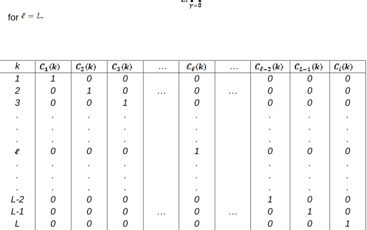
where is denoted as activation coefficient and it is defined as indicate (6) and (7) in Table 1:
for k … … 1 2 3 . . . . . . L-2 L-1 L 1 0 0 . . . 0 . . . 0 0 0 0 1 0 . . . 0 . . . 0 0 0 0 0 1 . . . 0 . . . 0 0 0 … … 0 0 0 . . . 1 . . . 0 0 0 … … 0 0 0 . . . 0 . . . 1 0 0 0 0 0 . . . 0 . . . 0 1 0 0 0 0 . . . 0 . . . 0 0 1
Table 1: Relation between the activation coefficients and the k parameter.
Table 1 shows that according with (6) and (7), when and otherwise . The mathematical formulation (5) can be seen as a collection of all the line equations of the segments involved in a PWL curve. The coefficients are included with the purpose of selecting a specific line equation for a
k value. A more detailed explanation for the ID-model can be found in [9]-[10].
2.1 Condensed ID-model form
The ID-model (5) describes a one-dimensional PWL curve as a sum of independent linear systems, where each system represents the line equation for any constitutive segment. Observe that in order to assure the continuity between two segments, the ended-segment coordinate of a -th segment, must be repeated as the start-segment coordinate for the -th segment. A condensed form for (5) can be obtained if all the
coordinates are collected in a unique coordinate matrix and all the linear systems are formed by picking out from this matrix, the coordinates belonging to any specific segment. This selection can be done if the activation coefficients are combined appropriately. The condensed form for the one-dimensional ID-model is given as follows:
(8)
where the -coefficients are given by
(9) (10) (11)
It is important to point out that both ID-model forms, the extended (5) and the condensed (8), are equally efficient from a computation point of view because for any value only one linear equation system will be active. The condensed form is in fact, only a shorter nomenclature for the extended ID-model.
3. DC analysis in PWL electrical networks
Finding all the operating points in PWL networks is a topic of interest in nonlinear circuit theory. The solution of this problem implies solving an equilibrium system ,
where x and y are described by PWL mathematical formulations. These formulations define a PWL curve by a function compound by a collection of linear mappings for each segment. Each mapping is only valid in a certain subspace or region that is bounded by line equations called hyperplanes. The hyperplanes are frontiers located on the curve breakpoints that make partitions over all the domain space of the PWL function.
For a one-dimensional PWL curve compound by segments, will be
hyperplanes and a set of regions for each n-th PWL element included in the network. So, in order to achieve the DC analysis in a network containing N-PWL elements, the number of regions to be analyzed will be [11]-[12]. It means a large number of regions and therefore a hard computational effort. Because a PWL function might have a solution in every region any method which claims to find all solutions must necessarily scan through all possible regions. Hence it is worthwhile to develop methods which can reduce the computational effort of this task [13].
The regions in a PWL curve which describes an n-th element are denoted as element regions and the set of regions obtained by the combination of all element regions are denominated as hyperplane partition regions. In this sense, the element regions and the hyperplane partition regions that contribute in the occurrence of any operating point will be denoted as DC element regions and DC solution regions, respectively.
4. A procedure for finding DC element regions
The procedure that is presented in this section lets discarding element regions that do not participate in any DC solution. It represents a great advantage because it makes possible that only such element regions involved in the occurrence of any operating point be taken into count. The procedure is also general because it does not depend of any specific PWL model description. In fact, the nonlinear elements are described by PWL curves defined as a set of graphic coordinates.
Although the procedure that will be exposed in this section can also be expanded in order to compute all the operating points, here it only will be used as a qualitative graphical tool for identifying DC element regions. The procedure for finding DC element regions can be summarized in the following steps:
1. An equlibrium equation system is obtained from figure 1. It is achieved by applying Kirchhoff laws.
2. is recast into the following representation
(12)
where
For
3. The nonlinear elements are described by PWL curves compound by segments. These curves are defined as a set of coordinates given by
It is important to note that will be as many sets as PWL elements existing in the network .
4. The coordinates of the n-th set are evaluated into (12). It will result in
sets of modified PWL curves or equation systems. These modified curves are defined as follows
(14)
for .
Each one of the elements of is obtained by substituting the -coordinates into and solving the system for the rest of - variables. Because of the N
elements are defined by one-dimensional PWL curves, then every element will involve 2 variables . It implies the existence of N equations and variables in (12) and therefore the two following cases:
Case .
For this case, the substitution into (12) always will produce a consistent system, it means, the same amount of equations and variables. Here, the computation of from can be obtained directly.
Case .
For this case, the substitution into (12) will produce an inconsistent system because always will be a greater amount of variables than equations. To overcome that problem, the network is analyzed by considering only two arbitrary PWL elements (pivot elements) simultaneously. The complementary PWL elements are replaced with Norton or Thevenin equivalents for each one of the element regions. Then the resulting circuit is submitted by an iterative process of all element region combinations. In every iteration, the DC element regions of the pivot elements are determined. It avoids the necessity of scanning all the possible element region combinations. As a result, a computational saving is obtained because a great amount of combinations can discarded.
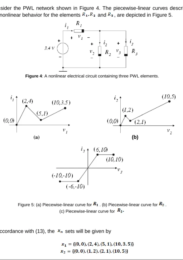
4.1 Example 1
Consider the PWL network shown in Figure 4. The piecewise-linear curves describing the nonlinear behavior for the elements and , are depicted in Figure 5.
Figure 4: A nonlinear electrical circuit containing three PWL elements.
(a) (b)
(c)
Figure 5: (a) Piecewise-linear curve for . (b) Piecewise-linear curve for . (c) Piecewise-linear curve for
In accordance with (13), the sets will be given by
(15) (16)
(17)
After applying Kirchhoff laws to Figure 4, the following equilibrium equation system is obtained:
(18)
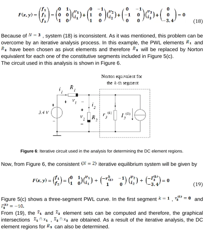
Because of , system (18) is inconsistent. As it was mentioned, this problem can be overcome by an iterative analysis process. In this example, the PWL elements and have been chosen as pivot elements and therefore will be replaced by Norton equivalent for each one of the constitutive segments included in Figure 5(c).
The circuit used in this analysis is shown in Figure 6.
Figure 6: Iterative circuit used in the analysis for determining the DC element regions.
Now, from Figure 6, the consistent iterative equilibrium system will be given by
(19)
Figure 5(c) shows a three-segment PWL curve. In the first segment , and From (19), the and element sets can be computed and therefore, the graphical intersections , are obtained. As a result of the iterative analysis, the DC element regions for can also be determined.
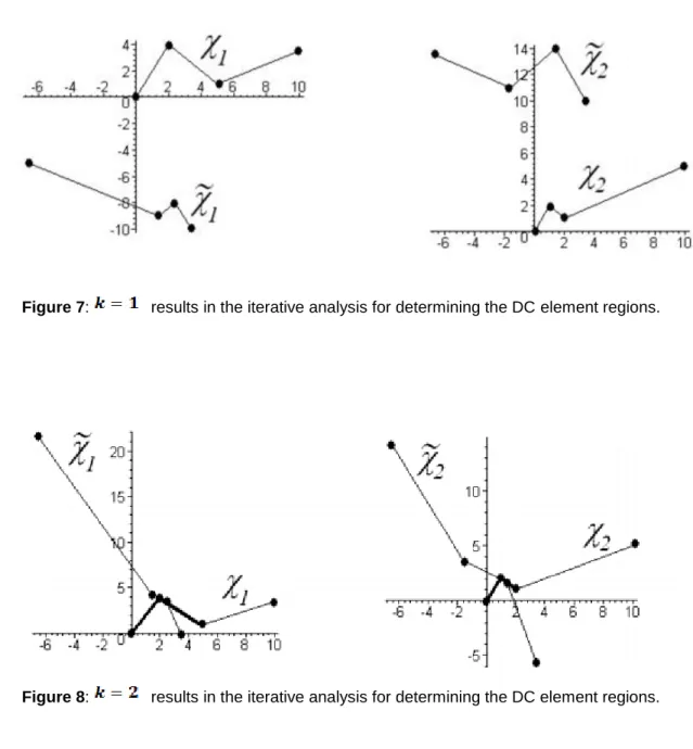
The results in this iterative analysis are reported in Figures (7)-(9).
Figure 7: results in the iterative analysis for determining the DC element regions.
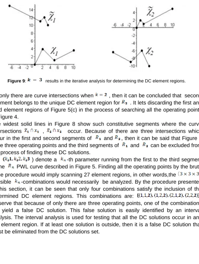
Figure 9: results in the iterative analysis for determining the DC element regions.
As only there are curve intersections when , then it can be concluded that second segment belongs to the unique DC element region for . It lets discarding the first and third element regions of Figure 5(c) in the process of searching all the operating points of Figure 4.
The widest solid lines in Figure 8 show such constitutive segments where the curve intersections , occur. Because of there are three intersections which occur in the first and second segments of and , then it can be said that Figure 4 have three operating points and the third segments of and can be excluded from the process of finding these DC solutions.
Let ) denote a -th parameter running from the first to the third segment in the PWL curve described in Figure 5. Finding all the operating points by the brute force procedure would imply scanning 27 element regions, in other words,the
possible -combinations would necessarily be analyzed. By the procedure presented in this section, it can be seen that only four combinations satisfy the inclusion of the determined DC element regions. This combinations are: . Observe that because of only there are three operating points, one of the combinations will yield a false DC solution. This false solution is easily identified by an interval analysis. The interval analysis is used for testing that all the DC solutions occur in any DC element region. If at least one solution is outside, then it is a false DC solution that must be eliminated from the DC solutions set.
5. Methodology for finding all the operating points
Given a nonlinear circuit containing N-PWL elements which are defined by ID-model descriptions, the following methodology can be applied for finding all the operating points.
1. By applying Kirchhoff laws, obtain the equilibrium equation system into the form (12).
2. Define the n-th PWL element (for n=1,2,…,N) by ID model as follows
in the extended form(5), or
(21)
in the condensed form (8).
The parameter denotes the -th segment belonging to any PWL curve it also indicates a specific region for an n-th PWL element.
3. Determine the DC element regions. It means finding all the element regions (the -values) involved in the occurrence of any operating point.
4. Knowing the specific element regions that must be considered in the DC analysis, the equilibrium system (12) is solved by considering all these -value combinations. This process always assures to achieving a consistent linear system for each combination. It is demonstrated by considering the number of equations and variables as follows:
Number of equations = 4N:
N linear equations from the equilibrium system.
Number of variables = 4N: N variables
N variables .
2N variables .
5. Finally, if it is necessary, the numerical results for the variables must be tested by interval analysis in order to discard false DC solutions.
Conclusions
An iterative-decomposed one-dimensional PWL model was presented. The model includes independent and dependent variables not coupled (decomposed) with graphic coordinates as parameters. A methodology for finding all the operating points in PWL electrical circuits was proposed. It includes a graphical procedure based on curve intersections for identifying the DC element regions and DC solution regions. It represents an important result because it avoids the need of testing all the regions produced by the combination of element regions.
References
[1] Le Jiayong, Pileggi Larry, Devgan Anirudh, Circuit Simulation of Nanotechnology Devices with Non-monotonic I-V Characteristics, ICCAD, San Jose California, USA, 2003.
[2] Sukhwany Bharat, Padmanabhan Uday, M. Wang Janet, Nano-Sim: A step Wise Equivalent Conductance based Statiscal Simulator for Nanotechnology Circuit Design, Proceedings of the Design, Automation and Test in Europe Conference and Exhibition, Electrical and Computer Engineering, University of Arizona, Tucson, 2005.
[3] Chua Leon O., Deng An-Chang, Canonical Piecewise-Linear Modeling, IEEE, Transactions on Circuits and Systems, VOL. CAS-33, May, 1986.
[4] Chua Leon O., Ying Robin L.P. Canonical Piecewise-Linear Analysis, IEEE, Transactions on Circuits and Systems, VOL. CAS-30, March, 1983.
[5] Chua Leon O., Ying Robin L.P.,Finding all solutions of piecewise-linear circuits, IEEE, Circuit Theory and Applications, VOL. 10, pp 201-229, 1982.
[6] Julian Pedro Marcelo, A High Level Canonical Piecewise-Linear Representation: Theory and Applications, Doctoral Thesis, Universidad Nacional del Sur, Argentina, 1989.
[7] Kevenaar Tom A. M., Leenaerts Domine M.W., A Comparison of Piecewise-Linear Model Description, IEEE, Transactions on Circuit and Systems-I, VOL. 30, NO. 12, December, 1992.
[8] van Bokhoven Wim M. G., Piecewise Linear Modelling and Analysis, Academic Press, 1998.
[9] Jimenez-Fernandez Victor, Hernandez-Martinez Luis and Sarmiento Reyes Arturo, An iterative decomposed piecewise-linear representation, XII IBERCHIP Workshop, San Jose de Costa Rica, March, 2006.
[10] Jimenez-Fernandez Victor, Hernandez-Martinez Luis and Sarmiento Reyes Arturo, Two dimensional piecewise-linear representation: an iterative-decomposed approach, IEEE International Caribbean Conference on Devices, Circuits and Systems, ICCDCS-06, Playa del Carmen Mexico, April, 2006.
[11] Hasler M., On the number of solutions of piecewise-linear resistive circuits, IEEE, Transactions on Circuits and Systems, VOL. 36, pages 393-402, 1989.
[12] Nishi T., On the number of solutions of a class of nonlinear resistive circuits, IEEE, Transactions on Circuits and Systems, pages 766-769, 1991.
[13]Jimenez-Fernandez Victor, Hernandez-Martinez Luis and Sarmiento Reyes Arturo, A method for finding the DC solution regions in piecewise-linear networks, IEEE International Symposium on Circuits and Systems ISCAS-06, Kos Island Greece, May, 2006.