In Proc. ACM SIGGRAPH, pp. 443-450, July 1994.
Partitioning and Ordering
Large Radiosity Computations
Seth Teller
†Celeste Fowler
†Thomas Funkhouser
?Pat Hanrahan
†Abstract
We describe a system that computes radiosity solutions for polyg-onal environments much larger than can be stored in main mem-ory. The solution is stored in and retrieved from a database as the computation proceeds. Our system is based on two ideas: the use of visibility oracles to find source and blocker surfaces potentially visible to a receiving surface; and the use of hierarchical tech-niques to represent interactions between large surfaces efficiently, and to represent the computed radiosity solution compactly. Vis-ibility information allows the environment to be partitioned into subsets, each containing all the information necessary to transfer light to a cluster of receiving polygons. Since the largest subset needed for any particular cluster is much smaller than the total size of the environment, these subset computations can be performed in much less memory than can classical or hierarchical radiosity. The computation is then ordered for further efficiency. Careful or-dering of energy transfers minimizes the number of database reads and writes. We report results from large solutions of unfurnished and furnished buildings, and show that our implementation’s ob-served running time scales nearly linearly with both local and global model complexity.
CR Categories and Subject Descriptors: I.3.7 [Computer Graphics]: Three-Dimensional Graphics and Realism –Radiosity; J.2 [Physical Sciences and Engineering]: Engineering.
Additional Key Words and Phrases: Multigridding; equilibrium
methods; spatial subdivision.
†Computer Science Dept., Princeton University, Princeton NJ 08544 ?AT&T Bell Laboratories, Murray Hill, NJ 07974
1
Introduction
An important application of computer graphics is the modeling of lighting in buildings. In fact, such interior lighting simulations are the major application of the radiosity method. Unfortunately, radiosity algorithms still are not fast and robust enough to handle standard building databases. Evidence of this is that previous radiosity images typically show a solution for only a single room of modest geometric complexity. Furthermore, “tricks” are often used to hide artifacts and to cope with even this low level of model complexity. In this paper we describe radiosity computations on very large databases.
There are three basic measures of the complexity of a radiosity solution: the input complexity, the output complexity, and the intermediate complexity.
• The input complexity is related to the number of geometric primitives, textures, and light sources present.
• The output complexity is related to the number and type of elements required to represent the computed radiosity solu-tion. Note that the output complexity is much, much greater than the input complexity, as it includes the input model plus a representation of the radiosity on all surfaces. The radiosity function may be very complex due to shadowing and lighting variations, and much recent research has con-cerned its compact, accurate representation. The optimal output complexity is that which represents the radiosity so-lution to within a specified error with a minimal amount of information.
• The intermediate complexity is related to the size of the data structure needed to perform the radiosity computation. The major components of the intermediate complexity are the form factor matrix and any data structures used to accel-erate visibility computations. Since the form factor matrix may grow quadratically in the output complexity, and since accelerated visibility queries may involve sophisticated data structures, the intermediate complexity may be even greater than the output complexity, and is, in fact, usually the lim-iting factor in performing large radiosity simulations. When storage is unlimited, the optimal intermediate complexity is that associated with the most rapidly converging iterative scheme.
Model Surfaces Patches Elements Time Theater [1] ∼5K ∼80K ∼1M 192 H
Mill [5] ∼30K ∼50K 195 H
Cathedral [28] ∼10K ∼75K 1 H Table 1: Previous complex radiosity solutions.
Several complex radiosity computations have been reported in the literature (Table 1). Perhaps the most complex is the Candle-stick Theater reported in Baum et al [1]. This simulation gener-ated over a million elements, performed 1600 iterations of a pro-gressive refinement algorithm (shooting from a single source), and took approximately 8 days to compute. Other reported complex radiosity simulations each generated less than 100,000 elements. Our goal is to render complete buildings at one square inch effec-tive resolution, obviously a very resource-intensive computation. For example, consider the model of the University of Califor-nia, Berkeley Computer Science Building. The furnished building model contains more than 8,000 light sources and 1.4 million sur-faces and requires approximately 350 megabytes of storage [9]. We estimate that 10 to 100 million elements may be required to represent a high-fidelity radiosity solution throughout the model.
Intermediate memory demands often determine the limits on the size of the model used in a radiosity system. The interme-diate memory usage depends on the representation of the form factor matrix. Two general approaches have emerged for cop-ing with the size of the form factor matrix: hierarchical radiosity
Figure 1: A locally dense,
globally sparse interaction block matrix.
and visibility subspaces. Hierarchical radiosity (and its relative, wavelet radiosity) efficiently approximate form factor matrices in situations where a set of large surfaces are mutually visible. Tech-niques are only recently emerging for handling large numbers of small, mutually visible surfaces, for example by clustering. The problem of efficiently computing cluster-cluster interactions is not addressed in this paper. However, our visibility subspace meth-ods do exploit the fact that in many environments, particularly building interiors, only a small percentage of the environment is visible from any particular surface. A global visibility precompu-tation constructs this potentially visible set for each surface, and the subspace methods maintain the set throughout hierarchical re-finement.
Figure 1 depicts a sparse block-structured form factor matrix. Each diagonal block represents a dense interaction within a cluster of surfaces, e.g., the polygons comprising a room. Each off-diagonal block represents the coupling between these clusters, e.g. the rooms visible from a given room. Thus each block is locally dense, but the matrix is globally sparse.
In this paper we describe our system to compute radiosity so-lutions in such environments. The environment is assumed to be very large and hence is stored in a database as the computation proceeds. The ensuing radiosity computation is partitioned into subsets. Each subset contains the information needed to perform a transfer of light to a cluster of polygons. These subset com-putations are ordered to perform the light transfers efficiently by reducing the number of database reads and writes. We report the results of simulations run for models of varying density (local complexity) and overall size (global complexity).
This system is built upon previously described hierarchical radiosity methods, global and local visibility algorithms, and database and walkthrough implementations.
2
Prior Work
The problem of increasing the speed and accuracy of radiosity solutions has been addressed on many fronts.
• Visibility. One of the most expensive operations in global
illumination is visibility computation. For a given surface, the set of surfaces that illuminate (or are illuminated by) it must be efficiently identified. Clearly this requires global knowledge of the model.
Classical radiosity algorithms used a “hemicube” algorithm to approximate each surface’s occluded view of the model as an environment map onto faces of a cube centered on a surface point [6]. The projection operation involved the whole model and respected depth, producing discretized sur-face fragments visible to the sample point. This and other point-sampling techniques (e.g., [4]) may not detect relevant light sources and/or blockers, however.
Shaft culling recast global visibility into a collection of vis-ibility subspaces by generating a common shaft volume for each interacting pair, and treating as blockers only those
ob-jects (potentially) intersecting the shaft [14, 18]. Finally, preprocessing and incremental maintenance techniques used a coherent global pass through the model to generate initial blocker lists, then maintained the lists incrementally under link subdivision [25]. These techniques, in contrast to those based on point-sampling, are conservative in the sense that they never wrongly exclude a blocker or light source from an interaction.
• Solution Methods. Classical radiosity algorithms generate
a row-diagonally dominant interaction matrix [6]. The ra-diosity matrix equation is then solved by repeatedly updat-ing the matrix entries usupdat-ing a numerical solution technique, typically Gauss-Seidel iteration. Several proposed improve-ments address the order in which the matrix entries are up-dated. Progressive radiosity techniques choose sources in brightness order and shoot their energy into the environment [5]. This may involve considerable bookkeeping, since each shoot updates many brightnesses, and the relative priorities of queued shooters may change considerably. Parallel imple-mentations of progressive refinement have been reported [2, 19]. “Super-shoot gather” techniques repeatedly (over)shoot from and gather to a small number of surfaces, ignoring any interactions not involving the shooters [7, 12].
• Hierarchical Approaches and Clustering. Matrix-based
solutions consider the matrix at a single granularity, namely the correspondence between each matrix entry and pair of surfaces in the environment. The hierarchical radiosity algo-rithm applied techniques developed for then-body problem, incorporating a global error bound and allowing surfaces to exchange energy whenever they could do so within the spec-ified error [15]. Thus, wherever sufficiently far-apart or dim surfaces interact, hierarchical methods essentially compact a block of the form-factor matrix into a scalar. Recursive application of this idea yielded a radiosity algorithm with running time that grows linearly with the number of out-put elements. The hierarchical radiosity algorithm did not address the “clustering” problem of efficiently handling in-teractions among surfaces composed of many small surfaces; some techniques have been recently proposed to do so [20, 22, 29].
• Meshing and Finite Element Methods. Finally, meshing
and finite-element techniques have been employed to im-prove the accuracy of radiosity solutions. Classical and hi-erarchical solution algorithms represented radiosity as con-stant over each surface. Galerkin-based methods use finite element techniques to represent radiosities more generally, as weighted sums of smoothly varying basis functions de-fined over each surface [16, 17, 27, 30]. The resulting so-lutions have better smoothness and convergence behavior than those of classical radiosity. Recently, the wavelet ra-diosity method [13, 21] combined hierarchical rara-diosity with Galerkin techniques.
3
Basic Ideas
Our system is based on two ideas: partitioning and ordering.
Partitioning decomposes the database into subsets. Each
sub-set contains the information needed to gather all the energy des-tined for a cluster of receivers. We assume that the largest subset, including the sources, receivers, and visibility and interaction in-formation, requires fewer resources than would be required for the whole model. Performing energy transfers for a partition amounts to a single block iteration of an iterative solution of the radios-ity system of equations. Partitioning is implemented by finding those clusters of source polygons visible to a cluster of receiving
polygons. Only light originating from the sources may directly illuminate the receivers. Furthermore, only polygons visible to the
receivers may block light transfers from the sources. Therefore,
the visibility and light transfer computations may use the same database.
The goal of partitioning is to reduce the solver’s working set to a manageable size. Receiver clusters may have dense interac-tions in a local region, but should have sparse interacinterac-tions with the remainder of the environment. Our implementation inherits clustering information (and thus local density) from the modeling hierarchy, and achieves global sparseness by partitioning accord-ing to visibility.
Ordering is scheduling radiosity subcomputations –the energy
transfers– to achieve rapid convergence. An example of an order-ing algorithm is the progressive radiosity algorithm, in which the source with the largest unshot radiosity is selected to “shoot” its energy into the environment. In our system, the order must also be chosen so that the memory “footprint” changes slowly; that is, the working set needed for the next transfer should differ little from that of the current transfer. Successful ordering strategies reduce the read and write traffic of the working set from and to external storage, while maintaining rapid convergence properties. In this paper we analyze several methods for ordering the en-ergy transfers: random order; model definition order; source order; and spatial cell order. We also briefly discuss optimal orderings.
4
System Architecture
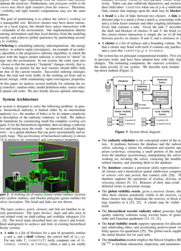
Our system is designed to solve the following problem: in prac-tice, hierarchical radiosity is limited either by its intermediate complexity (i.e., the number of links) or by its output complexity (the description of the radiosity solution), or both. We address both limitations by constructing small but complete working sets (Figure 2) for the hierarchical algorithm, then invoking a radiosity solver and storing away the result – an improved, typically larger, answer – in a spatial database that can grow incrementally and ar-bitrarily large. This partitioning of hierarchical radiosity is shown in§5 to preserve its correctness and convergence properties.
Figure 2: A working set of source cluster (white outline), receiver
cluster (yellow outline), and blocker polygons (green outline) for a solver invocation. The braid and links are not shown.
The types surface, patch, element, and link are familiar to ra-diosity practitioners. The types blocker, shaft, and tube arise in recent related work on shaft-culling and visibility subspaces [14, 18, 25]. The novel types described here are clusters and braids, defined analogously to surfaces and links in existing hierarchical radiosity systems.
• A tube is a list of blockers for a pair of geometric entities
pand q, and a shaft volume, the convex hull of (p∪q). For any tube T, variety(T) lazily computes one of in-visible, visible, or partial, when p and q are totally
mutually invisible, visible, or only partially visible, respec-tively. Tubes can also subdivide themselves and reclassify their child tubes’varietieswhen one ofporqsubdivides. Only entities that impinge upon the shaft may be blockers. • A braid is a list of links between two clusters. A link is a directed edge to a patchpfrom a patchq, associating withp
andqa form factor estimate and other coupling information. Every link contains a tube. Given the tube T describing the shaft and blockers of clusters R and S, the braid over this cluster-cluster interaction is simply the set of all links between patches in clustersRandS, and a reference toT. • A cluster is a list of surfaces and a bounding volume. Note that a cluster may braid with itself if contains any patchesp
andqsuch thatvariety(p, q)6=invisible.
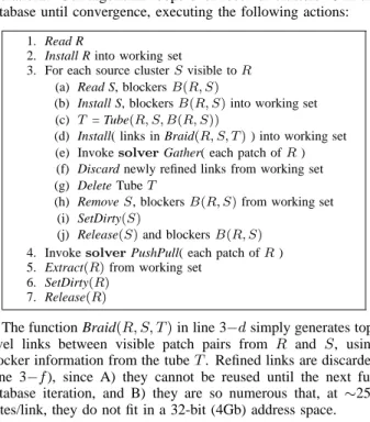
The system has six principal computational modules. Five exist in previous work, and have been adopted here with only slight changes. The remaining component, the radiosity scheduler, is the main novelty of our system. We describe each module in top-down fashion (Figure 3).
DISK Database Clusters Radiosity Scheduler !? ! Local Visibility Oracle Radiosity Solver ? Blocker Lists Global Visibility Oracle ? Computation Storage A directs B A queries B ! ? Shafts Subdivision Spatial (elements, links ) B B A A A writes to B A reads from B B B A A Working Set
Figure 3: System block diagram.
• The radiosity scheduler is the conceptual center of the sys-tem. It mediates between the database and the radiosity solver, selecting a cluster for refinement and transfer oper-ations (ordering), extracting a small portion of the model from the database (partitioning), manipulating the solver’s working set, invoking the solver, extracting the modified, refined clusters, and returning them to the database. • The database contains a persistent (disk) representation of
all clusters and a hierarchical spatial subdivision comprised of convex cells and portals that connect cells [26]. The database supports the operations of reading, dirtying, and
releasing clusters [9, 11]. Releases of dirty data result in
deferred writes to persistent storage.
• The global visibility oracle, given a receiver cluster, iden-tifies those clusters potentially visible to the receiver, i.e., those clusters that may illuminate the receiver, or block en-ergy transfers to it [23, 25]. A cluster may be visible to itself.
• The hierarchical wavelet radiosity solver generates high-quality radiosity solutions using wavelet bases of general order and Gaussian quadrature [13, 15, 21].
• The local visibility oracle supports operations for allocating and subdividing tubes, and accelerating point-to-point visi-bility queries for quadrature [25]. The global oracle supplies the initial blocker list for each tube.
• The visualization module employs the Silicon Graphics IRIS GLtmto facilitate interaction, inspection, and animation of
geometric data structures and algorithms [24]. It has proven indispensable to developing a working system.
5
Partitioning
We wish to partition a huge radiosity computation into a sequence of small gathers to individual receivers, each of which can fit into a small amount of memory. What information must be maintained in order to schedule and perform each gather correctly? Clearly the receiver and source cluster involved must be memory resident, as must their braid (links) and blocker polygons (cf. Figure 2). We compile this working set for each transfer, and supply it to the radiosity solver.
Our system constructs partitioning information from three sources. First, the modeling instantiation hierarchy yields clus-ters of polygons that separately comprise the structural elements, furnishings, light fixtures, etc., of the model. Second, a spa-tial subdivision groups clusters into cells by proximity, separating them along major sources of occlusion. Third, a visibility com-putation identifies all cluster pairs that may exchange energy [11, 23, 26].
The final tool is a flexible database from which individual por-tions of the model may be extracted, modified and replaced [11]. We adapted the database to support the new datatypes required for radiosity.
5.1 The Algorithm
Our algorithm: extracts each receiver and its visible set from the spatial database; links them; refines and gathers across the links; and returns the modified clusters to the database. A hierarchi-cal wavelet radiosity solver performs the refinement and gather operations. Our algorithm loops over receiver clusters R in the database until convergence, executing the following actions:
1. Read R
2. Install R into working set
3. For each source clusterSvisible toR
(a) Read S, blockersB(R, S)
(b) Install S, blockersB(R, S)into working set (c) T = Tube(R, S, B(R, S))
(d) Install( links in Braid(R, S, T)) into working set (e) InvokesolverGather( each patch ofR) (f) Discard newly refined links from working set (g) Delete TubeT
(h) RemoveS, blockersB(R, S)from working set (i) SetDirty(S)
(j) Release(S)and blockersB(R, S)
4. InvokesolverPushPull( each patch ofR) 5. Extract(R)from working set
6. SetDirty(R)
7. Release(R)
The function Braid(R, S, T)in line 3−dsimply generates top-level links between visible patch pairs from R and S, using blocker information from the tubeT. Refined links are discarded (line 3−f), since A) they cannot be reused until the next full database iteration, and B) they are so numerous that, at ∼250 bytes/link, they do not fit in a 32-bit (4Gb) address space.
5.2 Iteration Methods, Correctness, and Convergence
Hierarchical radiosity performs Jacobi iteration. That is, only af-ter a complete update of all patch’s gather slots are any patch’s shoot slots updated (by Push and Pull [15]). Jacobi iteration is clearly an untenable strategy for extremely large models, since it would necessitate reading and writing every patch twice per up-date. Moreover, hierarchical radiosity is often memory-bound in
practice, i.e., limited by the number and computational complexity of its active set of links, or by the size of the solution in progress. Our partitioning scheme eliminates Jacobi iteration altogether, and entirely removes the memory limitations on hierarchical radiosity for environments of sufficiently limited visibility.
The correctness of the partitioned solver is easily shown. Dur-ing any gather to a clusterR, the only patches excluded as sources areinvisiblefromR, and therefore cannot affect the computed solution onR.
The convergence of the partitioned solver follows from a nu-merical argument. The scheduler solves the radiosity matrix equa-tion as does tradiequa-tional hierarchical radiosity, but for one differ-ence: each receiver sees a combination of old and updated shoot slots on other clusters, rather than seeing uniformly old slots. The scheduler is therefore performing Gauss-Seidel iteration of the lin-ear system, rather than Jacobi iteration as in hierarchical radiosity. Since both methods converge for row-diagonally dominant sys-tems of radiosity equations [6], convergence of the partitioning algorithm is assured.
5.3 Partitioning Results
We studied the performance of our system for models of varying complexity. In one test, we increased local complexity using mod-els Office, Office Low, and Office High which represent the same office without furniture, with coarsely modeled furniture, and with very detailed furniture. These three models contain roughly one hundred, fifteen hundred, and thirty-five hundred input patches, respectively. In a second test, we increased global complexity using the unfurnished models Office, Floor, and Building which represent an office, one entire floor of a building, and finally an entire five floor building (including an atrium and many offices, open areas, stairwells, and classrooms). These models contain roughly one hundred, seven thousand, and forty thousand input patches, respectively. Gather 0 2 4 6 8 10 12 14 Working Set (Mb)
Figure 4: Working set size while solving the Building model.
We measured the input, intermediate, and output complexity, as well as working set memory requirements, for solutions of these test models. Statistics for three complete iterations (gathers to all clusters) of the radiosity solver are shown in Tables 2 and 3. The minimum allowable element area was one square inch for all runs. All times are wall-clock measurements using a 16µ-sec timer, on a lightly loaded SGI Crimson Reality Engine with a 50 MHz R4000 CPU, 256Mb memory, and 8Gb local disk. Figure 4 charts the size of the solver working set during one full iteration of the most complex model, Building.
Several trends can be gleaned from the measurements. First, the visibility and hierarchical radiosity techniques compacted large numbers of potential elements and interactions to manageable sizes. Second, partitioning techniques successfully bounded the working set size at a few tens of megabytes, even for models de-manding several gigabytes of intermediate solution data. Third, intermediate and output complexity and running time appear to vary nearly linearly with input complexity. Thus, partitioning
Input Intermediate Output Observed
Working Set(Mb) # Links # Elements Elapsed Time (s) Model Clusters / Patches / Lights WS Total WS Total / Patch WS Total / Patch Total / Patch
Office 36 127 18 1.3 9.5 3,914 36,186 285 1,445 3,142 24.7 180 1.4
Office Low 70 1,418 21 11.1 239.9 38,593 960,432 677 7,081 36,377 25.7 7,111 5.0 Office High 70 3,466 21 14.1 414.4 48,784 1,678,105 484 8,975 42,400 12.2 13,051 3.8 Table 2: Input, intermediate, and output complexities, and observed solution times, for models of increasing local complexity. The
tabulated quantities are divided into: WS (the largest working set processed by the solver); Total (the total data processed throughout the run); and Per Patch (the total amount divided by the number of input patches). The intermediate working set WS was defined as the size of the links (including tubes, shafts, and kernel coefficients), elements (including wavelet coefficients), and blocker polygons.
Input Intermediate Output Observed
Working Set(Mb) # Links # Elements Elapsed Time (s) Model Clusters / Patches / Lights WS Total WS Total / Patch WS Total / Patch Total / Patch
Office 36 127 18 1.3 9.5 3,914 36,186 285 1,445 3,142 24.7 180 1.4
Floor 1,761 7,054 788 3.7 1,116.1 12,532 4,307,705 611 2,686 250,933 35.6 56,712 8.0 Building 9,625 39,979 7,826 14.5 6,063.0 52,454 23,528,943 589 7,104 1,265,843 31.7 491,040 12.2
Table 3: Input, intermediate, and output complexities, and observed solution times, for models of increasing global complexity.
successfully exploited the global sparsity of the interaction ma-trix to achieve radiosity solutions for very large models, while maintaining quite small working sets.
6
Ordering
Partitioning alone is not sufficient to produce a practical system for large radiosity solutions. The partitioned transfers must be
ordered so as to minimize expensive reads and writes of partial
solution data from and to the database.
To be effective, an ordering algorithm must schedule successive gathers so as to minimize disk accesses, while maintaining rapid convergence properties. Much work has focused on the effects of ordering on convergence rates for the radiosity computation [5, 7, 12]; here we concentrate on the effect of ordering on disk accesses.
A good ordering algorithm maintains a high degree of coher-ence among the working sets of successive cluster interactions. Unfortunately, finding an optimal ordering is intractable. The problem is computationally equivalent to finding a solution to the traveling salesman problem. As a practical simplification, we have considered only orderings in which all gathers to a single cluster are performed successively (i.e., complete gathers). These order-ings are particularly efficient and easy to implement because all sources and blockers for a complete gather to a single cluster are contained in the gatherer’s visible set. Our implementation reads the entire set of clusters visible from the gatherer into the memory resident cache before performing any transfers to the gatherer.
We experimented with several ordering algorithms: • Random order gathers to clusters in random order. • Model order gathers to clusters in the order in which they
were instantiated by the modeler. In most cases, this is not a random order since models are often constructed by successive addition of related parts. For instance, in the Berkeley Computer Science building model, walls, ceilings and floors were instantiated first (grouped roughly by room), followed by patches representing light fixtures and furniture. • Source order gathers to that cluster which has most often
acted as a source (ties are broken by proximity to the most recent gatherer). This strategy is based on the intuition that the working set of a cluster that has been visible to many
previous receivers is likely to have a large overlap with the current working set.
• Cell order schedules clusters by traversing cells of the
wall-aligned BSP-tree [8] spatial subdivision [23, 26]. Consec-utive cells are chosen by selecting the neighbor cell whose intervening boundary has the largest transparent area. This approach exploits the visibility coherence of clusters due to proximity and local intervisibility.
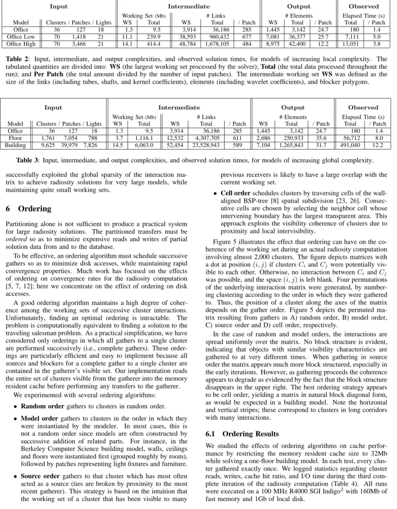
Figure 5 illustrates the effect that ordering can have on the co-herence of the working set during an actual radiosity computation involving almost 2,000 clusters. The figure depicts matrices with a dot at position(i, j)if clustersCiandCj were potentially vis-ible to each other. Otherwise, no interaction betweenCi andCj was possible, and the space(i, j)is left blank. Four permutations of the underlying interaction matrix were generated, by number-ing clusternumber-ing accordnumber-ing to the order in which they were gathered to. Thus, the position of a cluster along the axes of the matrix depends on the gather order. Figure 5 depicts the permuted ma-trix resulting from gathers in A) random order, B) model order, C) source order and D) cell order, respectively.
In the case of random and model orders, the interactions are spread uniformly over the matrix. No block structure is evident, indicating that objects with similar visibility characteristics are gathered to at very different times. When gathering in source order the matrix appears much more block structured, especially in the early iterations. However, as gathering proceeds the coherence appears to degrade as evidenced by the fact that the block structure disappears in the upper right. The best ordering strategy appears to be cell order, yielding a matrix in natural block diagonal form, as would be expected in a building model. Note the horizontal and vertical stripes; these correspond to clusters in long corridors with many interactions.
6.1 Ordering Results
We studied the effects of ordering algorithms on cache perfor-mance by restricting the memory resident cache size to 32Mb while solving a one-floor building model. In each test, every clus-ter gathered exactly once. We logged statistics regarding clusclus-ter reads, writes, cache hit ratio, and I/O time during the third com-plete iteration of the radiosity computation (Table 4). All runs were executed on a 100 MHz R4000 SGI Indigo2with 160Mb of fast memory and 1Gb of local disk.
A) Random B) Model C) Source D) Cell
Figure 5: Matrices depicting permutations of the cluster-cluster interaction matrix. A dot at position(i, j)denotes potential intervisibility ofCiandCj. Cluster position along axes corresponds to gather order during a complete radiosity iteration in A) random order, B) model order, C) source order, and D) cell order.
Clusters Mb Cache I/O Total Order Read Read Hit Ratio Time(s) Time(s) Random 77,916 4,374 35.4% 23,330 49,111 Model 44,163 2,376 63.4% 12,806 43,685 Source 30,798 1,708 74.4% 8,912 33,815 Cell 11,312 617 90.6% 3,180 26,454 Table 4: I/O statistics for various ordering algorithms.
There are significant differences in the I/O overhead incurred by each ordering algorithm. Figure 6 shows the percentage of total execution time spent on I/O (transfers between the disk and mem-ory resident cache) for different gather orders. Random order had a 35.4% cache hit ratio, spending 23,330 seconds (47.5% of the total execution time) on more than 4.3GB of I/O between the disk and memory resident cache. In contrast, cell ordering achieved a 90.6% hit ratio, spending only 3,180 seconds on I/O (12.0% of the execution time). We conclude that the order in which clusters are processed can greatly affect performance during radiosity compu-tations on very large models. We are currently investigating other possible ordering algorithms, including ones derived from pro-gressive radiosity [5], nearest neighbors, and minimum spanning trees [3]. We expect that the best ordering algorithms will take into account both cache coherence and convergence behavior.
Random Model Source Cell
Gather Order 0 10000 20000 30000 40000
Elapsed Time (seconds)
Solver I/0
Figure 6: Time distributions for various gather orders.
7
Results
•=⇒
Using a Silicon Graphics Crimson workstation with a single 50 MHz processor and 256 megabytes of main memory, we computed three complete iterations of a radiosity solution on the entire un-furnished Berkeley Computer Science Building model to one inch resolution. The input model had 9,625 clusters comprising a total of 39,979 polygons. Of these polygons, 7,826 were emissive and served as light sources.
To give an idea of scale, the total area of all polygons in the un-furnished building model is 64,517,972 square inches. Therefore,
without the use of visibility-based partitioning and hierarchical techniques, the numbers of elements and links potentially created during the radiosity computation at one inch resolution are approx-imately6.4×107 and4.2
×1015, respectively – unmanageably
high.
Statistics regarding the time and space complexity of the radios-ity solution for the entire unfurnished building model are shown in Table 5. To our knowledge, this is the most complex model for which a radiosity solution has been computed. The entire radios-ity computation took 136.4 hours and created 1,265,843 elements and 23,528,943 links – 2.0% and 0.00000056% of the potential numbers at one inch resolution, respectively. The partitioning techniques yielding a maximum working set size of 14.5MB, or 0.24% of the 6.1GB of total intermediate and output data. Cell ordering yielded a total I/O time of 14.2 hours, or 10.4% of the total execution time.
# # # Max Solver I/O Total
Iter Elements Links WS Time Time Time
0 39,979 - - - -
-1 295,039 2,649,521 2.0 3.3 0.2 5.1 2 884,905 15,860,111 11.2 40.6 3.2 47.0 3 1,265,843 23,528,943 14.5 69.9 10.8 84.3 Total 1,265,843 23,528,943 14.5 113.8 14.2 136.4 Table 5: Complexity of radiosity solution for the unfurnished
building model (times are in hours).
The five color plates on the next page show images of a ra-diosity solution for one furnished floor of the Berkeley Computer Science Building model, after two complete iterations. The solu-tion contains 734,665 elements and took 48.5 hours to compute. Plate I shows an overhead view of the furnished floor. Plates II and III show interior views of a typical furnished office, shaded and with an overlaid quadtree mesh, respectively. The global and local complexities of the radiosity solution are readily apparent from these views. Plates IV and V show a typical work area and hallway view, respectively.
The radiosity solutions generated by this system are used as input for the real-time walkthrough program (the color plates were generated using screen-captures from this program). The same visibility information and computations used to determine source and receiver interactions are used to maintain an interactive frame rate in the walkthrough. The hierarchical (quadtree) representation of radiosity on each polygon is particularly useful, as it allows easily selectable levels of detail [10] for each polygon.
Plate I. The entire furnished floor, solved to one inch effective resolution (734,665 elements).
Plate II: Office, gouraud shaded.
Plate IV: Workroom, gouraud shaded.
Plate III: Office, meshed.
8
Summary and Discussion
This paper presented a system that exploits visibility and coher-ence information to compute radiosity solutions for very large geometric databases, using existing high-quality global illumi-nation algorithms. Physically-based lighting simulation is more challenging than standard rendering algorithms in that the output complexity is very high, and the intermediate complexity and cal-culation costs are even higher. However, in the future there are likely to be many applications requiring display of complex, real-istic virtual environments, such as the building used in this study. To achieve such complexity requires advances at both the theoret-ical and the practtheoret-ical level. The theorettheoret-ical advances discussed in this paper are the visibility and hierarchical radiosity algorithms. The practical advances include the use of system techniques such as databases, scheduling, and caching.
Specifically, we have implemented a system capable of com-puting radiosity solutions from large models residing in a database stored on a disk. We show how partitioning the model leads to small working sets, allowing us to process databases much larger then those we could handle without partitioning. Poor partitioning of the database can cause it to be read and written many times. We show how clever ordering can significantly reduce disk traffic. The combination of these two techniques allow us to handle very large geometric models.
Given our experience with the system to date, the follow-ing research directions seem promisfollow-ing. First, the tradeoffs be-tween gathering and shooting algorithms in hierarchical radiosity should be investigated, as preliminary results indicate that shoot-ing converges more rapidly in some situations. Second, interac-tions among objects comprised of many small polygons must be handled more efficiently, perhaps by incorporating the notion of levels of detail into the radiosity solution method. Third, the vis-ibility calculations used to determine soft shadows are still very expensive, and should be improved. Finally, the refinement or-acle employed by the hierarchical radiosity algorithm is far too conservative. Rather than relying solely on estimates of form fac-tor and transport error, it should incorporate a term based upon representation error over each receiver surface.
Acknowledgments
Carlo Séquin founded the Building Walkthrough Group at Berke-ley, and generously shared the latest model of Berkeley’s (now-built) Computer Science Building, Soda Hall. David Laur’s help with system administration and color figures was indispensable. Peter Schröder contributed to a C++ reimplementation of the wavelet radiosity solver. Michael Cohen shared his insights about iterative radiosity solution methods. Finally, Dan Wallach helped with video production for the paper submission, and Tamara Mun-zner helped process statistics for the final version.
We are grateful to the National Science Foundation (contract No. CCR 9207966) and to DIMACS for their support, and to Silicon Graphics, Forest Baskett, and Jim Clark for their gift of a Reality Engine.tm
References
[1] Baum, D., Mann, S., Smith, K., and Winget, J. Making Radiosity Usable: Automatic Preprocessing and Meshing Techniques for the Generation of Accurate Radiosity Solutions. Computer Graphics (Proc. Siggraph ’91) 25, 4 (1991), 51–60.
[2] Baum, D., and Winget, J. Real Time Radiosity Through Parallel Pro-cessing and Hardware Acceleration. Computer Graphics (1990 Symposium on
Interactive 3D Graphics) 24, 2 (March 1990), 67–75.
[3] Bentley, J.Experiments on Geometric Traveling Salesman Heuristics. Tech. Rep. Computing Science (No. 151), AT&T Bell Laboratories, 1990. [4] Campbell III, A., and Fussell, D.Adaptive Mesh Generation for Global
Diffuse Illumination. Computer Graphics (Proc. Siggraph ’90) 24, 4 (1990), 155–164.
[5] Cohen, M., Chen, S., Wallace, J., and Greenberg, D. A Pro-gressive Refinement Approach to Fast Radiosity Image Generation. Computer
Graphics (Proc. Siggraph ’88) 22, 4 (1988), 75–84.
[6] Cohen, M., and Greenberg, D. The Hemi-Cube: A Radiosity Solution for Complex Environments. Computer Graphics (Proc. Siggraph ’85) 19, 3 (1985), 31–40.
[7] Feda, M., and Purgathofer, W.Accelerating radiosity by overshooting. In Proc.3rdEurographics Workshop on Rendering (May 1992), pp. 21–31.
[8] Fuchs, H., Kedem, Z., and Naylor, B.Predetermining visibility priority in 3-D scenes. Computer Graphics (Proc. Siggraph ’79) 13, 2 (1979), 175–182. [9] Funkhouser, T. Database and Display Algorithms for Interactive Visual-ization of Architectural Models. PhD thesis, (Also TR UCB/CSD 93/771) CS
Dept., UC Berkeley, 1993.
[10] Funkhouser, T., and S´equin, C. Adaptive display algorithm for in-teractive frame rates during visualization of complex virtual environments.
Computer Graphics (Proc. Siggraph ’93) 27 (1993), 247–254.
[11] Funkhouser, T., S´equin, C., and Teller, S.Management of Large Amounts of Data in Interactive Building Walkthroughs. In Proc. 1992
Work-shop on Interactive 3D Graphics (1992), pp. 11–20.
[12] Gortler, S., Cohen, M., and Slusallek, P.Radiosity and relaxation methods – Progressive refinement in Southwell relaxation. Technical Report TR-408-93, Department of Computer Science, Princeton University, 1993. [13] Gortler, S., Schr¨oder, P., Cohen, M., and Hanrahan, P.Wavelet
radiosity. Computer Graphics (Proc. Siggraph ’93) (August 1993), 221–230. [14] Haines, E., and Wallace, J. Shaft Culling for Efficient Ray-Traced
Radiosity. In Proc. 2ndEurographics Workshop on Rendering (May 1991).
[15] Hanrahan, P., Salzman, D., and Aupperle, L.A Rapid Hierarchical Radiosity Algorithm. Computer Graphics (Proc. Siggraph ’91) 25, 4 (1991), 197–206.
[16] Heckbert, P., and Winget, J. Finite element methods for global illu-mination. Tech. Rep. UCB/CSD 91/643, CS Department, UC Berkeley, 1991. [17] Lischinski, D., Tampieri, F., and Greenberg, D. P.Combining Hier-archical Radiosity and Discontinuity Meshing. Computer Graphics (Proc.
Sig-graph ’93) 27 (1993).
[18] Marks, J., Walsh, R., Christensen, J., and Friedell, M. Image and Intervisibility Coherence in Rendering. In Proc. of Graphics Interface ’90 (May 1990), pp. 17–30.
[19] Recker, R., George, D., and Greenberg, D.Acceleration Techniques for Progressive Refinement Radiosity. Computer Graphics (1990 Symp. on
Interactive 3D Graphics) 24, 2 (1990), 59–66.
[20] Rushmeier, H., Patterson, C., and Veerasamy, A.Geometric sim-plification for indirect illumination calculations. In Proc. Graphics Interface
’93 (1993), pp. 227–236.
[21] Schr¨oder, P., Gortler, S., Cohen, M., and Hanrahan, P.Wavelet projections for radiosity. In Eurographics Workshop on Rendering (1993), pp. 105–114.
[22] Smits, B., Arvo, J., and Greenberg, D. A Clustering Algorithm for Radiosity in Complex Environments. Computer Graphics (Proc. Siggraph ’94)
28 (1994).
[23] Teller, S. Visibility Computations in Densely Occluded Polyhedral Envi-ronments. PhD thesis, (Also TR UCB/CSD 92/708) CS Dept., UC Berkeley,
1992.
[24] Teller, S. A Methodology for Geometric Algorithm Development. In
Proc. Computer Graphics International ’93 (1993), N. and D. Thalmann,
Eds., pp. 306–317.
[25] Teller, S., and Hanrahan, P. Global Visibility Algorithms for Illu-mination Computations. Computer Graphics (Proc. Siggraph ’93) 27 (1993), 239–246.
[26] Teller, S., and S´equin, C. H. Visibility Preprocessing for Interactive Walkthroughs. Computer Graphics (Proc. Siggraph ’91) 25, 4 (1991), 61–69. [27] Troutman, R., and Max, N. Radiosity algorithms using higher order
finite element methods. Computer Graphics (Proc. Siggraph ’93) (1993), 209– 212.
[28] Wallace, J., Elmquist, K., and Haines, E.A Ray Tracing Algorithm for Progressive Radiosity. Computer Graphics (Proc. Siggraph ’89) 23, 3
(1989), 315–324.
[29] Xu, H., Peng, Q.-S., and Liang, Y.-D. Accelerated radiosity method for complex environments. Computers and Graphics 14, 1 (1990), 65–71. [30] Zatz, H. Galerkin radiosity: A higher order solution method for global