EDHEC RISK AND ASSET
MANAGEMENT RESEARCH CENTRE 393-400 promenade des Anglais 06202 Nice Cedex 3
Tel.: +33 (0)4 93 18 32 53 E-mail: [email protected] Web: www.edhec-risk.com
Static Allocation Decisions in the
Presence of Portfolio Insurance
Felix Goltz
Senior Research Engineer, EDHEC Risk and Asset Management Research Centre
Lionel Martellini
Professor of Finance and Scientific Director of the EDHEC Risk and Asset Management Research Centre
Koray D. Simsek
2
Abstract
This paper attemps to determine what fraction a static investor should optimally allocate to investment strategies with convex exposure to stock market returns in a general economy with stochastically time-varying interest rates and stock market excess returns. The results obtained using Monte Carlo analysis show that investors should allocate between 45% and 63% of their portfolio to such portfolio insurance strategies. Moreover, the inclusion of portfolio insurance strategies leads to important utility gains. Our results are robust with respect to the choice of the objective, the presence of realistic levels of market friction, heterogeneous expectations on volatility, and various parametric assumptions.
We would like to thank Noël Amenc, Alain Dubois, Frank Fabozzi, Yves Lehman and John Mulvey for very useful comments. All remaining errors, if any, are ours.
EDHEC is one of the top five business schools in France. Its reputation is built on the high quality of its faculty (110 professors and researchers from France and abroad) and the privileged relationship with professionals that the school has cultivated since its establishment in 1906. EDHEC Business School has decided to draw on its extensive knowledge of the professional environment and has therefore focused its research on themes that satisfy the needs of professionals.
EDHEC pursues an active research policy in the field of finance. The EDHEC Risk and Asset Management Research Centre carries out numerous research programmes in the areas of asset allocation and risk management in both the traditional and alternative investment universes.
Introduction
Dynamic investment strategies, which provide non-linear (convex) exposure to stock market returns, have seen tremendous growth over the past decade. This paper analyses the optimal static allocation to such investment strategies in a Monte-Carlo framework.
The salient characteristic of such portfolio insurance products is the repackaging of strategies that involve long and short positions in derivatives and/or the underlying asset into an investment vehicle that is easily accessible by investors under a static buy-and-hold format. Typically, such products are sold to investors in the form of derivatives (“certificates”) or investment funds (”structured funds”). Historically, the first occurrence of a strategy leading to non-linear payoffs in institutional money management was the introduction of constant proportion or option based portfolio insurance strategy (CPPI and OBPI). More recently, payoffs based on exotic derivatives have been introduced.
It has early been recognized that portfolio insurance strategies are natural investment choice for institutional investors, who have a particularly strong preference for non-linear payoffs because of the non-linear nature of the liability constraints they face (see Draper and Shimko (1993)). Leland (1980) has shown in a fairly general context that investors whose risk tolerance increases with wealth more rapidly than average will rationally wish to obtain portfolio insurance.1 This is the case in particular for institutional investors whose portfolio value must at all costs exceed a given value, but thereafter can accept reasonable risks. That rational investors should opt for portfolio insurance strategies raises an interesting question that is the focus of the present paper: what is the optimal allocation to portfolio insurance strategies and stocks and bonds?
Generally speaking, two different approaches to risk management exist. The first approach consists of diversification, i.e., reducing risk by optimal asset allocation techniques on the basis of imperfectly correlated assets. The second approach consists of hedging, i.e., reducing risk by using some form of insurance contract (or derivative instrument) on a given underlying asset. Given that diversification and hedging are two different, and perhaps competing, forms of risk management, the question remains whether combining these two approaches leads to any benefits. In particular, portfolio insurance products are often seen as stand-alone strategies, already providing risk reduction without a need for further diversification.
Of course, asset pricing theory allows us to better understand the nature of the relationship between allocation and hedging from a conceptual standpoint. It can be argued that portfolio insurance can be regarded as the most general, dynamic, as opposed to a static, form of asset allocation. It is indeed well known from Merton’s (1973) replicating argument interpretation of the Black and Scholes (1973) formula, that non-linear payoffs based on an underlying asset can be replicated by dynamic trading in the underlying asset and the risk-free asset.2 As a result, it appears that an investor willing and able to engage in dynamic asset allocation strategies will be in a situation to generate the most general form of risk management possible, and this encompasses both static diversification and dynamic hedging. While the benefits of dynamic asset allocation strategies in a stochastically time-varying environment have been recognized since the late 1970s (see Hakanson (1971) and Samuelson (1969), in a discrete-time setting, as well as Merton (1971), in a continuous-time setting), it is only recently that specific optimal asset allocation models that exhibit an explicit time-dependency in the presence of stochastic opportunity sets have been introduced.3
Given that a portfolio insurance strategies can be viewed as being some dynamic asset allocation strategy, investors may be able to enjoy the benefits of dynamic asset allocation strategies through the use of buy-and-hold investment in such products.4 In this paper, we focus on the benefits that
3 1 - Leland (1980) also shows that investors whose return expectations are more optimistic than average will also rationally wish to obtain portfolio insurance.
2 - An already mentioned example of use of dynamic asset allocation techniques to generate a structured product type of payoff is the CPPI technique, where dynamic rebalancing between the risky and risk-free asset is performed so as to guarantee a minimum capital at maturity.
4
can be gained by a myopic investor who is willing to expand the opportunity set so as to include structured products. The reason why we focus on the case of a myopic investor is twofold. First, most investors use static asset allocation in practice because they feel they lack the infrastructure and expertise necessary to the implementation of dynamic asset allocation strategies and are reluctant to face the associated costs.5 Second, it is precisely the focus of this paper to test whether investors might be able to enjoy the benefits of dynamic asset allocation strategies, while staying within the framework of static asset allocation
As such, our paper is closely related to a number of papers that look at optimal portfolios when investors have access to a risky asset and options on this risky asset. Under a set of rather stringent assumptions (continuous trading, absence of transaction costs, leverage or short-sales constraints, constant volatility and drift of the underlying asset, symmetric information), the introduction of structured products would not improve the welfare of investors. In particular, in a Black-Scholes setting with continuous-time trading and no transaction costs, assets generating non-linear payoffs are redundant because they can be replicated by dynamic trading in the underlying assets and the risk-free asset. As a result the optimal allocation to such assets is indeterminate when an investor’s expectation about parameter values matches those of the market, or infinite when the investor’s beliefs lead him to view the derivative asset as under-priced. On the other hand, any violation of the aforementioned assumptions would involve a trivial demand for non-linear payoffs. Because continuous trading is practically impossible and would be infinitely costly in the presence of transaction costs, several authors have examined the question of the optimal allocation to derivatives for investors who are prevented from performing dynamic trading. A first strand of the literature, initiated by Brennan and Solanki (1981), has examined the question of optimal positioning in derivatives assets from the static investor’s standpoint. The question is to determine the general shape of the non-linear function of the underlying asset that would generate the highest level of expected utility for a given investor. Carr and Madan (2001) extend this early work by considering optimal portfolios of a riskless asset, a risky asset and derivatives on the latter in an expected utility framework. They solve the asset allocation problem depending on the investor’s preferences, beliefs and market prices for an investor with increasing concave utility over final wealth. In a first step, they derive the optimal wealth as a function of the price of the risky asset, and then obtain the portfolio of the three assets that delivers the optimal wealth function.6 In that paper, the assumption of continuous-trading is replaced by the assumption of the existence of a continuum of call options with all possible strike prices, which allows static, as opposed to dynamic, replication of general non-linear payoffs.7 Also related are papers on optimal portfolio decisions with minimum target terminal wealth, including Grossman and Vila (1989), Cox and Huang (1989), Basak (1995, 2002), or Grossman and Zhou (1996), which rationalize particular portfolio insurance strategies. A second strand of the literature (starting with Leland (1980) and extended by Benninga and Blume (1985)) study the question from a different angle: taking as given a set of standard derivatives, these papers examine the features of (static) investors’ preferences that would support a rational non-zero holding of these contracts.
In this paper, we consider the question from yet a different perspective: in an incomplete market setup, we consider both the contract features and investors’ preferences as given and we obtain estimates of the optimal allocation to non-linear contracts. Simply put, the question we address is “how much to invest in portfolio insurance?”, as opposed to “who should buy portfolio insurance?”, or “what should portfolio insurance look like?”8
Our results suggest that the optimal fraction invested in portfolio insurance strategies takes on important magnitude, ranging from 45% to 63% for a typical investor. What is more, the inclusion 4 - Also see recent papers by Brandt et al. (2004) for interesting attempts at considering strategies aiming at exploiting returns predictability in the asset menu of a static investor.
5 - Other advantages of such strategies include privileged market access to derivatives (so-called "hidden assets") and mutualization benefits.
6 - Driessen and Maenhout (2003), in addition to the expected utility case, consider specific derivatives strategies for a variety of non-expected utility investors.
7 - See also Bookstaber et al. (1995), and Chan, Ching, and Yun (2004) for the portfolio problem in the presence of multiple risky assets and options on those assets, and Carr et al. (2003) and Liu and Pan (2003) for the case of a dynamic investor.
8 - Because our estimate for risk is a measure of downside risk, our work is also somewhat related to an early paper by Booth et al. (1985), who analyse stochastic dominance of portfolios using options. See also Ahn et al. (1999) for the optimal use of only put options or Dert and Oldenkamp (2000) for both put and call options in a downside risk context.
of portfolio insurance strategies allows for important utility gains through risk reduction. While the typical investor may increase her certainty equivalent 10-year return from 67% to 70%, the most-risk averse investor may increase the certainty equivalent return from 27% to 43% by including a portfolio insurance stratregy. We also gain insight into the robustness of optimal design analysis from our results. If the optimal allocation to portfolio insurance strategies is as significant as in our empirical results, even though their payoff structure is not necessarily optimal, this is a strong case for a positive impact of portfolio insurance on investor welfare. We also conduct a range of robustness tests that suggest that changes in setup do not alter our main conclusion on the impact of portfolio insurance strategies.
The remainder of the paper is organized as follows. Section 1 gives an overview of the type of portfolio insurance strategies that will be analyzed. Section 2 presents the framework in which we study the allocation benefits derived from including such assets. Section 3 provides base case empirical results, while a number of robustness checks are presented in section 4. Conclusions and suggestions for further research can be found in section 5. The details of the optimization program, as well as results for a different specification of preferences, appear in the appendix.
1. An Overview of Portfolio Insurance Strategies
While a wide range of different portfolio insurance products exist, we focus on products that are based on an equity index as the underlying asset. In an attempt to provide a rather exhaustive account of the portfolio insurance structures that exist in practice, we consider CPPI, standard OBPI as well as exotic OBPI structures. The focus on these forms of portfolio insurance is justified both from positive and normative arguments. From the positive side, it is the case that CPPI and OBPI products are the most common types of structures with non-linear payoffs offered to institutional investors. From the normative side, it can actually be shown that OBPI strategies are optimal strategies for an investor who is facing explicit constraints on terminal wealth where marginal indirect utility from wealth discontinuously jumps to infinity (Basak (1995) or Grossman and Vila (1989)), while CPPI strategies are optimal for an investor facing implicit wealth constraints, where marginal utility goes smoothly to infinity (see Basak (2002) for a discussion of explicit versus implicit wealth constraints).
1.1. OBPI
Starting with the example of a structure based on a simple European call option, we can write the payoff at maturity of the OBPI product as
S0 +k max S
(
T −S0,0)
Where S0 and ST denote the initial price of the stock market index and its price at expiration. In order to achieve this payoff, a portfolio P0 consisting of the following two components may be created:
(i) Pure discount bond investment of S0e−rT
(ii) European call option investment of kC0
Denote the Black-Scholes price of a European call option at time t as C( St,σ,r ,T ). Then the participation to the upside potential is given by
k = S0 −S0e
−rT
C( S0,σ,r ,T )
As long as the option price can be written in closed form, k may be written as an explicit function of parameter values. In the Black-Scholes case:
k = S0 −S0e
−Tr
S0N( d1)−S0e−rTN( d 2)
6
where d1 = ( r + σ
2/ 2)T
σ T , d2 =d1 − σ T and N .
( )
is the cumulative distribution function for astandardized normal distribution.
For a given maturity and initial asset price, k is a function of two parameters,σ, which affects the option price, and r , which affects both the option price and the present value of the guaranteed level. It is straightforward to see that ∂k / ∂σ <0 : the higher the volatility, the higher the value of the option. Its dependence on r seems to be more ambiguous since this parameter influences both the option price and the present value of the guaranteed level. On the one hand, as the interest rate increases, the price of the pure discount bond decreases, and more cash can be invested in the option. On the other hand, the price of the call option increases with r. However, the first effect always dominates the second, so for r > 0, ∂k / ∂r >0. It can also be shown that
0 ≤k ≤1.
1.2. Exotic OBPI
Various kinds of exotic options can be involved in the design of portfolio insurance products. A typical example involves an option paying off the maximum price that the underlying asset has reached during the period, i.e., S0 +k S
(
max −S0)
. This type of path-dependent option is known as a hindsight option. The payoff allows investors to capture price rises during the lifetime of the option as opposed to having a payoff that depends only on the price at maturity.In order to achieve this payoff, a portfolio P0 consisting of the following two components may be created:
(i) Pure discount bond investment of S0e−rT .
(ii) Hindsight call option investment of k HC0 .
The type of path dependency present in this product renders it more attractive and more expensive than the simple call option structure. With the same level of guaranteed capital, k will therefore be smaller than above. If we consider how k depends on the parametersσ and r , the reasoning for the portfolio insurance product including a plain vanilla call carries over to this path dependant portfolio insurance product. At initial date, the price of the hindsight option does not depend on
Smax since Smax =S0. In the context of a Black-Scholes economy, it can be shown (see Goldman,
Sosin, and Gatto (1979)) that the price of the hindsight option, denoted as HC ( S0,σ,r ,T ), is given by:9 HC( S0,σ,r ,T ) =S0e−rT N(b 1)− σ2 2r e Y2N( −b3) ⎛ ⎝⎜ ⎞ ⎠⎟ +S0e −T σ 2 2r N(−b2)−S0e −TN(b 2) where: b1 = ln( Smax / S0)+(−r + σ 2 2)T σ T , b 3 = ln( Smax / S0)+( r − σ2 2)T σ T , b2 =b1 − σ T , and Y2 = 2( r − σ 2 2)ln( S max / S0) σ2 .
As an explicit function for non-dividend paying stock, we have
k = S0 −S0e
−Tr
HC( S0,σ,r ,T )
For partial derivatives, one can verify in this case that ∂k / ∂σ <0, whereas ∂k / ∂r may take on positive or negative values.
In this paper, we focus on a discrete hindsight option, with payoff S0 +k max S
(
t −S0)
t=0 ,...,10 .
The only difference with the continuous version is that the price path is sampled at annual intervals. 9 - Goldman, Sosin, and Gatto (1979) derive the price of a lookback put option, which delivers a payoff of ( Smax−ST). The hindsight call option may be created by adding a position in a forward contract
and an amount of ( erT−1)S
10 - Throughout the paper, we assume a constant multiplier value. The method can easily be extended to allow for a time-varying multiplier value.
11 - Fama and French (1988) and Poterba and Summers (1988) were the first to provide empirical evidence of long-term mean reversion in stock returns. Barberis (2000), Wachter (2002), and Munk, Soerensen, and Nygaart (2004) derive solutions for optimal portfolio choice in the presence of mean reversion (driven by mean reversion in the dividend yield or the risk premium).
12 - In the presence of stochastic volatility, derivatives cannot be replicated by dynamic trading in the underlying asset and give access to new unspanned risk factors.
7 Therefore, intuition suggests that the price of this option is lower, hence k is higher than for the continuous version. At the same time, it is obvious that this type of option is more attractive than the simple call option from above; hence k is expected to be lower than with the plain vanilla call. Broadie, Glasserman, and Kou (1999) introduce correction terms that allow approximating the price of discrete options using closed-form solutions for their continuous counterparts. In our case the approximation error is large since the number of observations is small. Therefore, numerical procedures are preferable in order to estimate k (see section 3 below).
1.3. CPPI
Introduced by Black and Jones (1987) and Black and Perold (1992), the CPPI procedure allows the production of option-like positions through systematic trading rules. This procedure dynamically allocates total assets to a risky asset in proportion to a multiple of the cushion, i.e., the difference between current wealth and a desired protective floor. This produces an effect similar to owning a put option.
More formally, denote by Vt the portfolio value at date t, which is decomposed into the sum of two components, a floor, whose value is denoted by Ft, and a cushion, whose value is denoted by Ct. Then Vt=Ft+Ct. By definition, the floor value at any time t is given by Ft = kBt, where Bt is the value at time t of the risk-free asset, and k is the guaranteed level.
Let At be the amount invested in the risky asset (with value at time t denoted by St). At each decision date At=mCt, where m is the multiplier, while the remaining amount Vt-At is invested in the risk-free asset.10
2. Allocation Model
We consider a single-period stochastic optimization model with a time horizon of ten years. The assumptions are detailed below.
2.1. Assumptions on Preferences
The objective relate to a standard expected utility maximization program. We consider exponential utility defined by U W
( )
T =1−e−aWT , fora>0 , where a is the risk aversion parameter. Here
WT is the final wealth at the end of year 10, assuming the initial wealth is 1. We maximize the
expected utility for various values of a and then find the certainty equivalent in terms of a 10-year portfolio return, C, for the maximum expected utility zU*
: U
( )
1+C =E⎡⎣U W( )
T ⎤⎦ 1−e−a(1+C) =zU* ⇒C = − ln 1(
−zU*)
a −12.2. Assumptions on Asset Returns
The issue of modeling the future uncertainty is critical to any stochastic optimization problem. We choose to use stochastic differential equations (such as geometric Brownian motion) and to discretize them during the simulation of paths. Our model selection is driven by the goal to match the well-known empirical stylized facts of asset returns, including fat tails and mean reversion of returns.11 To this end, we define the data generating process by the following model with stochastic interest rate and stochastic volatility.12
dSt
St = μtdt+ Vt dWt
S
drt =a b
(
−rt)
dt+ σrdWtB8
dVt = κ θ −
(
Vt)
dt+ σV Vt dWt Vwhere St is the value of the underlying asset (stock index) at date t, rt is the (mean-reverting) value of the short-term rate at date t, Vt is the instantaneous variance of the log-returns for the stock, μt is the time-varying expected return on equity (to be specified below), W
S,
WB, and WVare correlated Brownian motions.13
It should be noted that in the stochastic volatility model the variance follows a square-root process, as in Heston (1993), and stochastic interest rates follow the Vasicek (1977) model. Our model is quite similar to the AFF1V model in Chernov et al. (2003), which, with constant drift, corresponds to the Heston (1993) model.
The short-term rate process we use conveniently allows for bond prices to be obtained in closed-form (see Vasicek 1977). It should be noted that the bond portfolio under consideration is a global bond index, which can be modeled as a zero-coupon bond with constant time-to-maturity τ , which we will set equal to ten years for the purposes of our analysis.
Btτ =exp −mtτ + 1 2 vt τ ⎡ ⎣⎢ ⎤ ⎦⎥ mtτ = βτ +( rt − β)1−e −aτ a vtτ = σr 2 2a3 1−e −aτ
(
)
2 + σr 2 a2 τ − 1−e−aτ a ⎛ ⎝⎜ ⎞ ⎠⎟where β is the risk-adjusted long-term value of the short-term rate, given by β =b− σrλB
a ,
with λB being the risk-premium associated to interest rate risk.
We may now specify the dynamics for the drift of the stock index. We first write down the market price of risk vector:
λS λB ⎛ ⎝⎜ ⎞ ⎠⎟ = σt S cov t dBtτ Bt τ , dStτ St τ ⎛ ⎝⎜ ⎞ ⎠⎟ covt dBtτ Bt τ , dStτ St τ ⎛ ⎝⎜ ⎞ ⎠⎟ σt B ⎛ ⎝ ⎜ ⎜ ⎜ ⎜⎜ ⎞ ⎠ ⎟ ⎟ ⎟ ⎟⎟ −1 μt S −rt μt B −rt ⎛ ⎝⎜ ⎞ ⎠⎟ where σt S = V
t is the volatility of stock returns, and σt
B the volatility of bond returns (see
below for more on the relationship between σt
B and σ r ). Equivalently, we have: μt S =rt + σt S λS +covt dBt τ Bt τ , dSt τ St τ ⎛ ⎝⎜ ⎞ ⎠⎟λB
Therefore, what we are interested in is the covariance of stock returns and bond returns. The bond price can be written as the following exponential function of the short rate:
Bt τ =K t Te−LtTrt where LtT =1−e −a T( −t) a
Using Ito’s lemma, we find that:
dBtτ Btτ = ∂B ∂t + ∂B ∂r a b
(
−rt)
+ 1 2 σ 2 ∂2B ∂r2 ⎡ ⎣⎢ ⎤ ⎦⎥dt + ∂B ∂r σrdWt B ≡ μt Bdt + σt BdW t B13 - For simplicity, we assume in what follows that WBand
where σt B = ∂B ∂r σr = − 1−e−a T( −t) a σr Finally, we have: μt S −rt = σt S λS + σt S σt B ρλB = σt S λS − 1−e−aτ a σrρλB ⎛ ⎝⎜ ⎞ ⎠⎟
Therefore, assuming constant market prices of equity and bond price risk, we obtain that the expected excess return on the equity index is given as a mean-reverting process because it is a linear function of the volatility process, which itself is assumed to be mean-reverting. Our setup is somewhat similar to Wachter (2000), who also has mean reversion in excess stock returns. There are, however, differences in the two models. On the conceptual standpoint, Wachter assumes a constant volatility so that the mean-reverting stochastically time-varying excess drift over the risk-free rate can rationalized only be by assuming a stochastic market price for risk. We take an opposite route by assuming a constant price for risk (λS ), and a stochastic quantity of risk (σt
S).
On the technical side, so as to maintain the assumption of a complete market setting, Wachter assumes a perfect negative correlation of the drift term and stock return, while we consider a more general framework with a correlation not necessarily equal to -1 (we take that correlation equal to -.77 in our base case).
2.3. Parameter Values
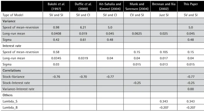
The model we use for stock and bond returns involves quite a few parameters. One approach would consist of estimating these parameters by fitting the model to historical data. Alternatively, we have chosen to select parameter values consistent with the existing literature. Table 1 contains information about related papers and the parameter values they use.
Table 1: Parameter Values. For Bakshi et al. (1997), the parameters are given on page 2018, under column All Options – SVSI. For Duffie et al. (2000), the parameters are given on page 1363, under column SV. For Ait-Sahalia and Kimmel (2004), the parameters are given on page 38, under column Daily. For Munk and Sørensen (2004), the parameters are given on page 2000, in Equation 32. For Brennan and Xia (2002), the parameters are given on page 1221, under column Estimate. SV stands for stochastic volatility, CI stands for constant interest rates and SI stands for stochastic interest rates. Initial values of variance and interest rate process are assumed to be equal to their long-run means, respectively, while the initial stock price is assumed to be 100.
For the parameters concerned with the variance process, we adopt the values in Ait-Sahalia and Kimmel (2004) who calibrate a Heston-type stochastic volatility model similar to the one we are using. The parameter values for the stochastic interest rate model are taken from Munk and Sorensen (2004) who use a Vasicek interest rate process that has been calibrated to fit historical
9 Bakshi et al. (1997) Duffie et al. (2000) Ait-Sahalia and Kimmel (2004) Munk and Sørensen (2004)
Brennan and Xia (2002)
This Paper
Type of Model SV and SI SV and CI SV and CI CV and SI Just SI SV and SI
Variance Speed of mean-reversion 0.98 6.21 5.0 5.0 Long-run mean 0.0408 0.019 0.045 0.0625 0.025 0.045 Sigma 0.42 0.61 0.48 0.48 Interest rate Speed of mean-reversion 0.58 0.15 0.105 0.15 Long-run mean 0.0345 0.0319 0.04 0.04 0.017 0.04 Sigma 0.03 0.015 0.013 0.015 Correlations Stock-Variance -0.76 -0.70 -0.77 -0.77 Stock-Interest rate -0.25 -0.25 Variance-Interest rate 0.00 Others Lambda_S 0.343 0.343 Lambda_B -0.207 -0.207
10
bond return behavior. Finally, the market prices of risk are taken from Brennan and Xia (2002) whose definitions for these parameters are identical to those of ours. For comparison purposes, we also show in table 1 parameter values in two papers using similar models, Bakshi et al. (1997) and Duffie et al. (2000).
Using these parameter values, which are depicted on the right-most column of table 1, we simulate 2500 paths.
2.4. Discretization Scheme and Optimization Program
The next step is the time-discretization of these processes, so that we can simulate paths. We adopt a Milstein discretization scheme, as described in Glasserman (2004). As opposed to a Euler scheme, it makes a difference in the discretization of the stochastic volatility process and helps us avoid negative variance values. Once the paths are simulated, returns for each asset class are calculated on each path in order to generate the scenarios. Then, we compute the return scenarios for the different portfolio insurance stratgies. For CPPI, this is simpler as we have the freedom of specifying the values for the parameters m and k, for which we choose 3 and 0.95, respectively. We also adopt weekly rebalancing. For standard and exotic OBPI (denoted by E-OBPI), first, we determine the respective values of k that correspond to these specific sets of scenarios. In other words, we determine the guarantee that can be offered for each structured product given the expectations about the economy. Similar to the method described in section 1.2, we price each option on the paths we simulate and find the matching values for k. Once this is done, we calculate the payoffs for each structured product using the formulas in section 1.2.
The scenarios for the total returns on each asset class are then fed to the optimization program. We consider four different sets of asset classes: a base case with stocks and bonds (No PI) and three more cases created with the addition of CPPI, OBPI, and E-OBPI respectively. As explained above, our specification of the objective function relies on maximizing the expected utility of the final wealth for the commonly used exponential utility function. We compute optimal portfolios for several values of the risk-aversion parameters (a) of the utility function. We plot the certainty equivalent wealth for each level of risk aversion.
3. Base Case Empirical Results
We first conduct base case experiments using the parameter values in table 1, and then perform a variety of robustness checks. We consider a typical allocation for an institutional investor’s portfolio with stocks/bonds of 51.6%/48.4%. This was obtained as an average of allocations by European and US institutions.14 We compare our solutions with this typical allocation at various stages of the analysis.15
In sections 3 and 4, before starting the optimal allocation exercise, we first calibrate the size of the payoff k to be consistent with the chosen parameter values (as explained in section 1). As a result, the portfolio insurance payoff is always fairly priced. This value turns out to be 0.8219 for standard OBPI and 0.5790 for the exotic OBPI.16
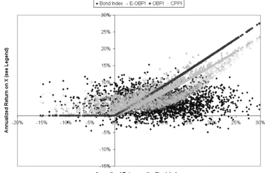
Figure 1 shows for each scenario the return for different asset classes against the stock index returns. The horizontal axis corresponds to the annualized return for the stock index while the vertical axis corresponds to annualized returns for other asset classes. As expected, the standard OBPI exhibits the kind of piece-wise linear convex payoff classic to call options. The exotic OBPI (E-OBPI) also exhibits a convex payoff indicating that a capital guarantee is provided. On the other hand, it dominates OBPI under scenarios with severe drops in the stock index, whereas OBPI can provide only a no-loss protection. Under optimistic scenarios, however, E-OBPI does not do as 14 - Bank of International Settlements (September 2003).
15 - Different estimates can be found in the literature. According to Davis (2003), an average UK (US) pension fund holds 71% (67%) equity and 29% (33%) fixed income securities. According to a recent survey of UK pension funds by Mercer Investment Consulting, the equity/bond mix is 65%/35%.
16 - Since the exotic OBPI can be described as a discrete hindsight option, it can be shown that this value is higher than the continuous hindsight, respectively. It is consistent to have a higher value for the standard OBPI, which can be described as a European call option.
well as OBPI. This is because of the higher cost, and hence lower upside potential, associated with the hindsight option, as opposed to the standard call option. Due to CPPI's being a guarantee as a function of the cash index (not the stock index), this non-linearity is somewhat less obvious. However, one can still observe the superior performance of CPPI over other portfolio insurance strategies in falling stock markets (left side of the chart).
Figure 1 – Annualized returns of several assets versus the annualized return on the stock index
Since we will see below that this property of CPPI returns has important consequences in terms of allocations, a few comments are in order. Among the three portfolio insurance strategies we implemented, OBPI and E-OBPI guarantee the initial investment, whereas CPPI guarantees 90% of the initial investment invested in the cash index (a natural result of CPPI being a dynamic mix of stocks and "cash"). The floor is constant with regards to this percentage, but not so in terms of dollars guaranteed. For the low stock return scenarios, we see that OBPI has a return of zero, whereas CPPI achieves positive returns in these scenarios. The main difference between OPBI and CPPI is that CPPI invests in (short term) cash whereas OBPI invests the present value of the guaranteed level into a 10-year zero coupon bond which gives CPPI's the possibility to outperform if the variation of interest rates is favourable.
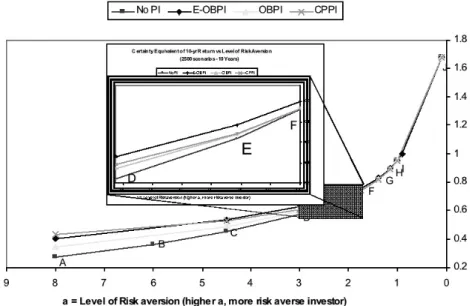
The results obtained for the optimal portfolios for expected utility maximisers are shown in figure 2. The certainty equivalent (expressed in terms of 10-year portfolio return) is computed for various levels of risk aversion (parameter a) and plotted for each set of asset classes. The presence of portfolio insurance improves the welfare of most investors (i.e., higher certainty equivalent return for the same value of a). For the most risk-averse investors, CPPI is the most attractive strategy, followed by the exotic OBPI. As the investor gets less risk averse, CPPI loses its appeal quickly and falls below the standard OBPI in the terms of certainty equivalent wealth, which is dominated by the exotic OBPI for all types of investors. For less risk-averse investors (several points on the right), standard OBPI and CPPI do not make a difference. Point E corresponds to the typical institutional investor whose degree of risk-aversion is given by a = 2.1775. For this risk-aversion level, the greatest improvement is achieved through exotic OBPI, which is followed by CPPI.
12
Figure 2 – Certainty equivalent plots for expected exponential utility maximization. The part that contains the typical investor’s level of risk aversion is magnified.
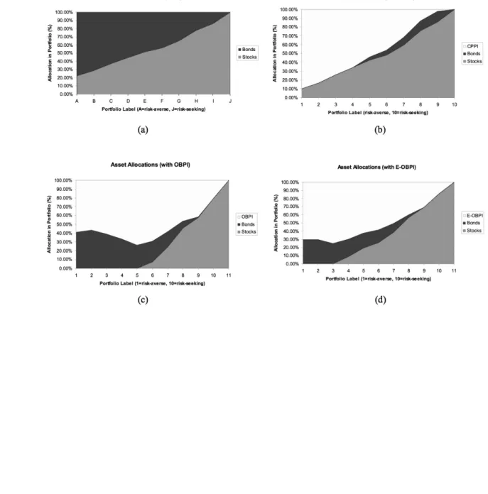
In figure 3, one may observe the change in asset allocation with respect to the change in the degree of risk aversion. These allocations correspond to points on the four lines in figure 4. As before, CPPI increases the expected utility by replacing the bonds in the portfolio. For low levels of risk aversion, it does not provide an improvement. Regardless of the degree of risk aversion, the exotic OBPI seems to have a greater presence in the optimal portfolios than the standard OBPI although their replacement behaviors in the portfolios are similar. In each of the three charts (b,c, and d), label 4 corresponds to the typical investor’s optimal portfolio, which corresponds to label E in the traditional asset universe (chart a). For this level of risk aversion, the optimal portfolios contain roughly the same proportion of portfolio insruance. In the case of CPPI, the rest of the optimal portfolio is dominated by stocks, whereas we see observe the opposite in the portfolio improved by the standard OBPI. The bond-stock allocation seems rather balanced in the optimal portfolio that contains the exotic OBPI. One final observation regarding the optimal portfolio allocations for the case of exponential utility maximization is that they are more reasonable (i.e., less dominated by portfolio insurance) than those in the mean-CVaR framework. This is obviously related to the fact that the focus on extreme risk embedded in Mean-CVaR optimization makes portfolio insurance particularly attractive.
We also conduct the same exercise for a different specification of the utility function, namely, power utility. Since the results are consistent with our findings for exponential utility, the description of this specification, as well as the results are delegated to an appendix.
In the next section, we will carry out various robustness analyses for the portfolio labeled 4 in figure 3(d). This corresponds to the optimal portfolio within the presence of an exotic OBPI structure for an exponential utility maximizing institutional investor whose typical allocation at the same risk aversion level is represented by portfolio E in figure 3(a), that is a=2.1775.
4. Extensions and Robustness Analysis
In the interest of brevity, we only present the robustness analysis with a focus on the exotic OBPI structure only. Similar results are available for the other objectives and insurance strategies, and can be obtained from the authors upon request.
4.1. Market Frictions
So far, we have assumed that there are no transaction costs and have chosen parameter values so as to make the product fairly priced (i.e., no profit for the provider of the portfolio insurance strategy) for a given size of the payoff (k). This has allowed us to focus on the optimal demand for structured products purely motivated by access to a non-linear payoff.
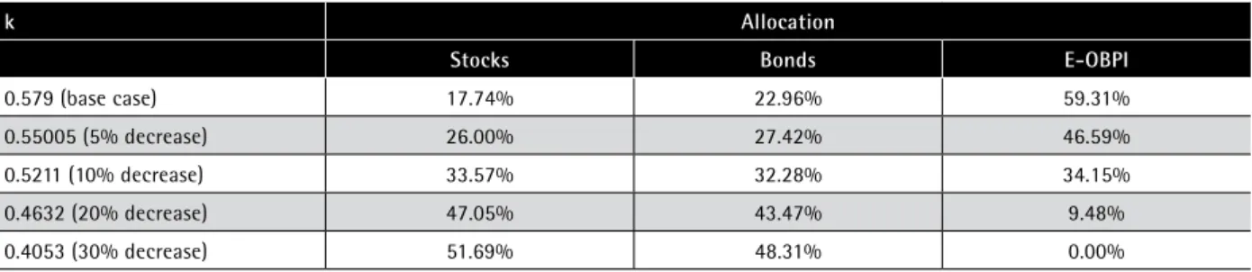
Because the introduction of market frictions leads to a decrease in the proposed level of exposure to the upside potential of the underlying index, we run the following stylized experiment.17 To test for the impact of market frictions, we reduce k by a fixed percentage, starting from the base case value k=0.579 all the way down to k=0.4053 (30% decrease with respect to base case). Accordingly, we update the payoff for the portfolio insurance product. Finally, we maximize the expected exponential utility at the same risk aversion level as portfolio 4 for various fee levels. The following table summarizes the results of this analysis. As a result of the market frictions, the allocation to portfolio insurance gradually decreases from 59.31% (base case). Though the impact of introducing these frictions is quite strong, the E-OBPI holding disappears from the optimal portfolio only when the participation (k) decreases by as much as 30%.
Table 2: Changes in the optimal asset allocation in the presence of frictions.
k Allocation
Stocks Bonds E-OBPI
0.579 (base case) 17.74% 22.96% 59.31%
0.55005 (5% decrease) 26.00% 27.42% 46.59%
0.5211 (10% decrease) 33.57% 32.28% 34.15%
0.4632 (20% decrease) 47.05% 43.47% 9.48%
0.4053 (30% decrease) 51.69% 48.31% 0.00%
4.2. Different Volatility Predictions
In this subsection, we do a comparative analysis of the parameter values for the volatility process to see how differences in opinions about these parameters impact investors’ appetite for portfolio insurance. In the presence of stochastically time-varying parameters, it can be argued that an investment in portfolio insurance offers an added advantage to investors since it allows them to gain an active exposure to rewarded sources of risks potentially different from the one implicit in stock and bond returns. For example, if volatility is stochastically time-varying, the inclusion of a OBPI product in an institutional investor’s asset allocation will induce a long position on volatility (position will make profit if volatility increases).
13 17 - Of course, in practice, frictions are not an add-on cost that can be measured as a percentage of k as modeled here for simplicity, and investors can only observe k as quoted by the bank..
14
To address how active views on volatility (i.e., deviations from market implied volatility) can affect the optimal allocation to portfolio insurance, we follow a two-step process: first, we select an optimal asset allocation when the portfolio insurance payoff is fairly priced, and then we see how heterogeneous expectations on volatility between the investor and the provider of portfolio insurance can induce a change in the allocation to these products.
For the first step, we choose our favorite portfolio, labeled 4 in figure 5. For the second step, we re-generate all the scenarios using a new value for the parameter θ, the long-term mean for volatility. However, we skip the step where we calibrate the k value. It is as if the original scenarios were generated by the provider of portfolio insurance (and therefore are used to determine k) and the new set were generated by the investor according to her expectations on volatility (and is therefore used to determine the optimal asset allocation). The following table summarizes our findings.
Table 4: Changes in the optimal asset allocation in the presence of heterogeneous expectations on volatility.
θ Allocation
Stocks Bonds E-OBPI
0.03 46.54% 26.64% 26.82%
0.045 (base) 17.74% 22.96% 59.31%
0.0625 0.00% 21.54% 78.46%
As expected, an investor endowed with a belief that the market’s ex-ante perception of volatility is lower than it should be will allocate more to portfolio insurance than in the base case, because the implied non-linear payoff seems to be underpriced. For example, if an investor has an active view stating that the long-term mean value for volatility should be 25% (corresponding to
θ =0.625), as opposed to the base case value 21.21% (corresponding to θ =0.045), then the upside potential k is higher than what it should be based on the investor’s prior, and portfolio insurance gets more attractive, which translates into an increase (from 59.31% to 78.46%) in the optimal weight.18 The results show that the damand due to a differing view on volatility is great with respect to the demand in the base case. At the same time, even when the investor expects lower volatility than the provider of portfolio insurance, the optimal holding E-OBPI holding remains important, which confirms the results from the analysis of frictions above.
4.3. Different Parameter Values
In what follows, we test for the impact of changes in the most important parameters, including speed of mean reversion, long-term volatility estimate, long-term risk-free rate, stock risk premia, etc. We test both the unrestricted case and the case when allocation to portfolio insurance is restricted to less than 20%.
In table 5, we first adjust the long-term value for interest rates, either down from 4% (base case) to 3% or up to 5%. As a result of these changes, the optimal allocation to bonds is naturally affected: given the mean-reversion feature of interest rates, an increase (decrease) in the long-term value signals a higher probability of future increase (decrease) in interest rates and therefore future decrease (increased) in bond prices, with a decreased (increase) allocation to bonds as a result.
Table 5: Changes in the optimal asset allocation as a result of changes in long-term value of interest rate level.
b Allocation
Stocks Bonds E-OBPI Expected 10-Yr
Return CE of 10-Yr Return
0.03 24.88% 27.84% 47.29% 1.0824 0.6540
0.04 (base) 17.74% 22.96% 59.31% 1.1750 0.7017
0.05 10.11% 18.63% 71.26% 1.2842 0.7529
In table 6, we conduct a similar analysis on the long-term value for stock index volatility (or actually variance), and adjust it either down from 4.5% (base case corresponding to 21.21% volatility) to 3% (i.e., 17.3205% volatility) or up to 6.25% (i.e., 25% volatility).
Table 6: Changes in the optimal asset allocation as a result of changes in long-term value of equity volatility level.
θ Allocation
Stocks Bonds E-OBPI Expected 10-Yr Return CE of 10-Yr Return
0.03 19.54% 13.94% 66.52% 1.1065 0.7090
0.045 (base) 17.74% 22.96% 59.31% 1.1750 0.7017
0.0625 15.43% 29.94% 54.63% 1.2280 0.6897
Table 7 shows the results for different values for the speed of mean-reversion to long-term stock index volatility (or actually variance), which is adjusted either down from 4 (base case) to 3 or up to 5.
Table 7: Changes in the optimal asset allocation as a result of changes in speed of mean-reversion in equity volatility.
κ(Kappa) Allocation
Stocks Bonds E-OBPI Expected 10-Yr
Return CE of 10-Yr Return
4.0 15.37% 21.56% 63.07% 1.1523 0.7006
5.0 (base) 17.74% 22.96% 59.31% 1.1750 0.7017
6.0 19.54% 24.01% 56.46% 1.1917 0.7025
Table 8 contains similar results on the long-term equity risk premium, which is adjusted either down from 0.343 (base case) to 0.3 or up to 0.4.
Table 8: Changes in the optimal asset allocation as a result of changes in equity risk premium level.
λs Allocation
Stocks Bonds E-OBPI Expected 10-Yr
Return CE of 10-Yr Return
0.300 11.06% 26.00% 62.94% 1.0102 0.6458
0.343 (base) 17.74% 22.96% 59.31% 1.1750 0.7017
0.400 26.03% 18.85% 55.11% 1.4404 0.7869
Overall, the impact of such changes does not appear to be significant in the sense that the fraction optimally invested in the E-OBPI strategy remains economically important in all cases.
The most dramatic change occurs when changing the long-term value for the long term interest rate level, which yields optimal holdings in the E-OBPI strategy ranging from 47% to 71%. Overall, our results display a comforting level of robustness with respect to the choice of parameter values.
5. Conclusions and Suggestions for Further Research
Our results show that a static investor should allocate a significant fraction of his wealth to portfolio insurance strategies. This optimal fraction takes on values ranging from 45% to 63% for a typical investor. The inclusion of these strategies allows for substancial utility gains, increasing the certainty equivalent 10-year return from 67% to 70% for the typical investor, and from 27% to 43% for the most risk averse investor. We argue that obtaining such significant optimal holdings in portfolio insurance strategies, whose payoff structure is not even necessarily optimal, makes a strong case for a positive impact of portfolio insurance on investor welfare. A range of robustness tests suggests that changes in our setup do not alter this conclusion.
16
Our work can be extended in two ways. It may be worthwhile to attempt to extend the early work on optimal demand for portfolio insurance (Brennan and Solanki (1981)) to path-dependent strategies, such as the E-OBPI strategy included in this paper. Our finding that the E-OBPI strategy is the preferred one for most levels of risk aversion for investors with either exponential or power utility can be taken as motivation to search for the general shape of the function of the underlying asset’s price path that would generate the highest level of expected utility. Another extension would be to focus on the presence of liability constraints and examine the impact of portfolio insurance strategies, or suitable extension of such strategies, on various types of pension plans.
References
• Ahn D., J. Boudoukh, M. Richardson and R. Whitelaw, 1999, Optimal Risk Management Using
Options, Journal of Finance, 54(1) 359-375.
• Ait-Sahalia, Y., and R. Kimmel, 2004, Maximum Likelihood Estimation of Stochastic Volatility
Models, Working Paper, Princeton University.
• Bakshi, G., C. Cao, and Z. Chen, 1997, Empirical Performance of Alternative Option Pricing
Models, Journal of Finance, 52, 2003-2049.
• Bansal, Ravi, Magnus Dahlquist and Campbell R. Harvey, 2004, Dynamic Trading Strategies and
Portfolio Choice, Working Paper, Duke University.
• Barberis, N, 2000, Investing for the Long Run When Returns Are Predictable, Journal of Finance,
55,1, 225-264.
• Basak, S., 1995, A General Equilibrium Model of Portfolio Insurance, Review of Financial Studies,
8, 1059-1090.
• Basak, S., 2002, A Comparative Study of Portfolio Insurance, Journal of Economic Dynamics and Control, 26, 7-8, 1217-1241.
• Benninga, S., and M. Blume, 1985, On the Optimality of Portfolio Insurance, Journal of Finance,
40, 1341-52.
• Black, F and Jones, R., 1987, Simplifying Portfolio Insurance, Journal of Portfolio Management,
Fall, 48-51.
• Black, F., and A. Perold, 1992, Theory of Constant Proportion Portfolio Insurance, Journal of
Economic Dynamics and Control, 16, 403-426.
• Black, F. and M. Scholes ,1973, Pricing of Options and Corporate Liabilities, Journal of Political
Economy, 81, 637-654.
• Bookstaber, R., and R. Clarke, 1983, An Algorithm to Calculate the Return Distribution of
Portfolios with Option Positions, Management Science, 4, 419-429.
• Booth J., H. Tehranian, and G. Trennepohl, 1985, Efficiency Analysis and Option Portfolio Selection,
Journal of Financial and Quantitative Analysis, 20(4), 435-449.
• Brandt, M. W., and P. Santa-Clara, 2006, Dynamic Portfolio Selection by Augmenting the Asset
Space, Journal of Finance, 61(5), 2187-2217.
• Brennan, M. J., and R. Solanki, 1981, Optimal Portfolio Insurance, Journal of Financial and
Quantitative Analysis 16, 279-300.
• Brennan, M.J., and Y. Xia, 2002, Dynamic Asset Allocation under Inflation, Journal of Finance,
57, 1201-1238.
• Broadie, Mark, Paul Glasserman, and S.G. Kou, 1999, Connecting Discrete and Continuous
Path-Dependent Options, Finance and Stochastics, 3, 55-82.
• Carr, P., and D. Madan, 2001, Optimal Positioning in derivative securities, Quantitative Finance,
1, 19-37.
• Carr, P., X. Jin and D. Madan, 2001, Optimal Investment in Derivative Securities, Finance and
Stochastics, 33-59.
• Chan, P, W. Ching and S. Yung, 2004, Optimal Strategies in Equity Securities and Derivatives,
Applied Mathematics and Computation.
• Chernov, M., A. R. Gallant, E. Ghysels and G. Tauchen, 2003, Alternative Models for Stock Price
Dynamics, Journal of Econometrics, 116, 225-257.
• Conze, Antoine and Viswanathan, 1991, Path Dependent Options: The Case of Lookback Options,
18
• Cox, J.C., and C.-F. Huang, 1989, Optimal Consumption and Portfolio Policies When Asset Prices
follow a Diffusion Process, Journal of Economic Theory, 49, 33-83.
• Davis, E, 2003, Institutional Investors, Financial Market Efficiency and Financial Stability, Working
Paper, Birbeck College.
• Dert C., and B. Oldenkamp, 2000, Optimal Guaranteed Return Portfolios and the Casino Effect,
Operations Research, 48, 768-775.
• Draper, D., and D. Shimko, 1993, On the Existence of ‘Redundant Securities’, University of
Southern California Working Paper.
• Driessen, J. and P. Maenhout, 2003, A Portfolio Perspective on Option Pricing Anomalies, working
paper, INSEAD.
• Duffie, D., K. Singleton, and J. Pan, 2000, Transform Analysis and Asset Pricing for Affine
Jump-Diffusions, Econometrica, 68, 1343-1376.
• Fama, E., and K. French, 1988, Dividend Yields and Expected Stock Returns, Journal of Financial
Economics.
• Glasserman, P., 2004, Monte Carlo Methods in Financial Engineering, Springer-Verlag, New
York.
• Goldman, B., H. Sosin, and M.A. Gatto, 1979, Path-Dependent Options: Buy at the Low, Sell at
the High, Journal of Finance, 34, 1111-1127.
• Grossman, S. J., and J-L. Vila, 1989, Portfolio Insurance in Complete Markets: a Note, Journal of
Business, 62, 473-476.
• Grossman, S. J., and Z. Zhou, 1996, Equilibrium Analysis of Portfolio Insurance, Journal of Finance,
11, 1379-1403.
• Hakanson, N. H., 1971, Multi-Period Mean-Variance Analysis: Toward a General Theory of Portfolio
Choice, Journal of Finance, 26, 857- 884.
• Heston, S. L., 1993, A Closed-Form Solution for Options with Stochastic Volatility with Applications
to Bond and Currency Options, The Review of Financial Studies 6(2), 327-343.
• Leland, H., 1980, Who Should Buy Portfolio Insurance?, Journal of Finance, 35, 581-94.
• Lioui, A., and P. Poncet, 2001, On Optimal Portfolio Choice under Stochastic Interest Rates, Journal of Economic Dynamics and Control, 25, 1841-1865.
• Liu, J., 1998, Portfolio Choice In Stochastic Environments, Stanford GSB working paper
• Liu, J., and J. Pan, 2003, Dynamic Derivative Strategies, Journal of Financial Economics,
forthcoming.
• Lynch, A., 2001, Portfolio Choice and Equity Characteristics: Characterizing the Hedging Demands
Induced by Return Predictability, Journal of Financial Economics 62, 67-130.
• Merton, R. C., 1971, Optimum Consumption and Portfolio Rules in a Continuous Time Model,
Journal of Economic Theory, 3, 373-413
• —,1973, Theory of Rational Option Pricing , Bell Journal of Economics and Management Science,
38,4, 141-183
• Munk, C. and C. Sorensen, 2004, Optimal Consumption and Investment Strategies with Stochastic
Interest Rates, Journal of Banking & Finance, 28, 1987-2013
• Munk, C., C. Sørensen, and T. Nygaart, 2004, Dynamic Asset Allocation under Mean-Reverting
Returns, Stochastic Interest Rates and Inflation Uncertainty, International Review of Economics & Finance, 13, 2, 141-166.
• Pelsser, A., and T. Vorst, 1995, Optimal Optioned Portfolios with Confidence Limits on Shortfall
Constraints, Advances in Quantitative Analysis of Finance and Accounting, 3A, 205-219.
• Poterba, S, and L. Summers, 1988, Mean Reversion in Stock Returns: Evidence and Implications,
Journal of Financial Economics.
• Samuelson, P., 1969, Lifetime Portfolio Selection by Dynamic Stochastic Programming, Review
of Economics and Statistics, 51, 239-246.
• Vasicek, O., 1977, An Equilibrium Characterization of the Term Structure, Journal of Financial
Economics, 5, 177-188.
• Wachter, J. A., 2002, Portfolio and Consumption Decisions under Mean Reverting Returns: An
Exact Solution for Complete Markets, Journal of Financial and Quantitative Analysis, 37,1, 63-91.
20
Appendix
A. Optimisation Model
For the optimization model, we define the following parameters and variables.
Parameters:
T Number of time periods
N Number of scenarios
P0 Initial value of the portfolio
Rt,Si
Total return on the stock index in period t under scenario i
Rt,Bi
Total return on the bond index in period t under scenario i
Rt,Gi
Total return on the guaranteed structured product in period t under scenario i
Variables:
wS Portfolio weight of stocks at the beginning
wB Portfolio weight of bonds at the beginning
wG Portfolio weight of guaranteed structured product at the beginning
PT,i Value of the portfolio at the end of period T under scenario i
rTP,i Rate of return for T periods on the portfolio under scenario i
Given these definitions, the optimization model can be formulated as follows: For exponential utility, the objective function is:
maximizemaximize 1 N 1−e −aPT i P0 ⎛ ⎝ ⎜ ⎜ ⎞ ⎠ ⎟ ⎟ i=1 N
∑
For power utility, we have, similarly: maximize maximize 1 N PTi P0 ⎛ ⎝ ⎜ ⎞ ⎠ ⎟ 1−b 1−b ⎛ ⎝ ⎜ ⎜ ⎜ ⎜ ⎜ ⎞ ⎠ ⎟ ⎟ ⎟ ⎟ ⎟ i=1 N
∑
For the special case of log-utility, we use: maximize maximize 1 N ln PTi P0 ⎛ ⎝ ⎜ ⎞ ⎠ ⎟ i=1 N
∑
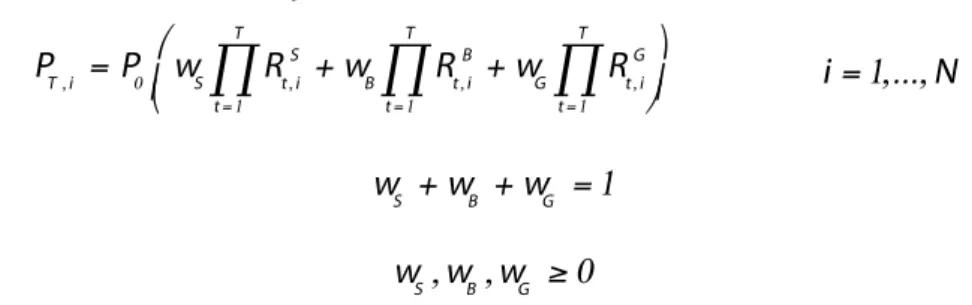
The respective maximization is subject to PT,i = P0 wS Rt,Si t=1 T
∏
+wB Rt,Bi t=1 T∏
+wG Rt,Gi t=1 T∏
⎛ ⎝⎜ ⎞ ⎠⎟ i=1,...,N wS +wB +wG =1 wS,wB,wG ≥0These constraints represent how we define the ending portfolio value and the 10-yr portfolio rate of return, respectively, for each scenario. We make sure that the portfolio weights add up to 1 and short sales are disallowed.
B. Expected Power Utility Maximisation
We also consider expected utility maximization with power utility defined by U W
( )
T =WT
( )
1−b 1−b , forwhere b ≥ 0 is the risk aversion parameter. Note that for b = 0 we have the expected wealth maxi-mizing investor and for b = 1 we have the investor with logarithmic utility. Again, we compute the certainty equivalent C as
U
( )
1+C =E⎡⎣U W( )
T ⎤⎦ 1+C(
)
1−b 1−b = zU * ⇒C =( )
1−b zU *(
)
1−1b−1As in the case of exponential utility, the certainty equivalent wealth is computed for various levels of risk-aversion (parameter b) and plotted for each set of asset classes in figure 6. Once again, the presence of portfolio insurance leads to improvements for most investors (i.e., higher certainty equivalent return for the same value of b). For the most risk-averse investors, CPPI is the most attractive strategy, followed by the exotic OBPI. As the investor gets less risk-averse, CPPI loses its appeal quickly and falls below the standard OBPI in the rankings, which is dominated by the exotic OBPI for most types of investors. The standard OBPI seems to be the best strategy for only one type of investor in our trials (b = 1.5). The special case of log-utility (b = 1) coincides with ex-pected wealth maximization (b = 1), which is an artifact of the buy-and-hold investment strategy. Once again, point E corresponds to the typical institutional investor whose degree of risk-aversion is given by b = 3.3213. For this risk-aversion level, the greatest improvement is achieved through exotic OBPI, which is followed by the standard OBPI.
Figure A1 – Certainty equivalent plots for expected power utility maximization. The part that contains the typical investor’s level of risk aversion is magnified.
22
Figure A2 shows the change in asset allocation with respect to the change in the degree of risk aversion. These allocations correspond to points on the four plots in figure A1. Overall, the evolution of the allocations with respect to thr risk aversion parameter are similar to the case of exponential utility. However, the weight invested in portfolio insurance strategies (i.e., their replacement impact) is higher for all levels of risk aversion, and especially for less risk-averse investors. In the case of OBPI, the optimal allocation of the less risk-averse investors now excludes bonds, whereas bonds are present in any but the least risk-averse portfolios in the exponential utility case. Compared to the mean-CVaR case, the benefits of portfolio isnurance are more pronounced for risk-seeking investors and less for risk-averse investors. In each of the three charts (b, c, and d), label 5 corresponds to the typical investor’s optimal portfolio, which corresponds to label E in the case without portfolio insurance (chart a).