Maximum Throughput Power Control
in CDMA Wireless Networks
Anastasios Giannoulis
Department of Electrical and Computer Engineering Rice University, Houston TX 77005, USA
Konstantinos P. Tsoukatos
Leandros Tassiulas
Communications and Computer Engineering Department University of Thessaly, Greece
Abstract— We introduce cross–layer, distributed power control algorithms that guarantee maximum possible data throughput in multihop CDMA wireless networks. Throughput maximization, for given power budget, is achieved by jointly performing dynamic routing and scheduling together with power control. The cross–layer interaction consists in differential queue length information, made available from the network layer, which is exploited by the physical layer power control function. The proposed back–pressure power control algorithms operate in real–time, i.e. in parallel with system evolution, and achieve maximum throughput without knowledge of traffic statistics. 1
I. INTRODUCTION
With the rapid growth of wireless networks, and the emer-gence of new high-rate applications, meeting efficiently de-mand in data rates is an important consideration. Taking full advantage of network resources will maximize user satisfac-tion, and increase network revenue.
Transmit power is a fundamental resource in wireless systems. In early work transmit power control was used to mitigate co-channel interference, by driving the signal-to-interference plus noise ratios (SINR) to predetermined target values [3]. This target tracking approach is appropriate for satisfying stringent quality of service (QoS) requirements of voice traffic. However, with the proliferation of wireless data, many applications are elastic in nature; they may operate under several different transmission rates, and hence tolerant to a wide range of SINR values. In the literature elastic QoS requirements are taken into account by formulating the power control problem in terms of utility functions (see e.g. [1], [9], [13]). Voice and data perceive different utilities, which reflect different degrees of user satisfaction, and typically depend on the transmission rates and power consumption. In a noncooperative game setting, selfish users individually adjust their powers in an effort to maximize their net utility (utility minus incurred cost). From a different, system–wide perspective, the goal is to employ power control as a means for optimizing the network’s aggregate utility. These two objectives may be difficult to reconcile. Even when the non-cooperative power control game leads to a Nash equilibrium this may be inefficient, i.e., it does not optimize aggregate network utility. Nevertheless, despite considerable previous
1This work was supported by the European Commission through the
EURONGI (specific research project RAWQOS) and NEWCOM Networks of Excellence, and by the ARO through grant W911NF-04-1-0306.
work ([1], [7], [9], [11], [13] and references therein), a clear understanding is still lacking as to how power control can be used to achieve the maximum possible data throughput in multihop wireless networks.
In this paper we propose distributed, maximum through-put power control algorithms. Throughthrough-put maximization is achieved by jointly performing dynamic routing and schedul-ing, together with power control. In the routing function, data find their way to the destination by back–pressure, i.e., following the direction of maximum differential backlog. Precisely this differential backlog information is then used to couple routing and scheduling with the power control function; this is an instance of cross–layer interaction. A prime advantage of the proposed back–pressure routing and power control algorithms is that they operate in real–time, i.e., they run in parallel with system evolution. The algorithms are in part distributed, as they rely on exchange of local backlog and interference information among neighboring nodes. Fur-thermore, they attain maximum throughput regardless of the statistics of network traffic. That is, functionality is ensured for unknown arrival rates, as long as these lie inside the system’s achievable throughput region. From a mathematical stand-point, the adopted maximum throughput formulation amounts to solving a global convex optimization problem at each time slot. However, in contrast to the standard deterministic approach, the system quantities are dynamic, i.e., they evolve over time, in parallel with the computations of the distributed algorithms. In spite of these stochastic fluctuations, the back– pressure routing and power control algorithms still succeed in providing maximum throughput.
The paper is organized as follows. Section II describes the wireless network model. In Section III we recall a policy that guarantees maximum throughput in general time–varying networks. In Section IV we present two maximum throughput, joint back–pressure routing, scheduling and power control algorithms, based on a best–response in a power control game, and a gradient method, respectively. Section V contains simulation results that illustrate the maximum throughput property of the proposed algorithms. Section VI concludes and points to extensions to this work.
II. SYSTEMMODEL
We consider a wireless ad-hoc network, consisting of N nodes. LetN be the set of all nodes, with cardinality|N |=N.
We denote byNi⊆ N, the set of nodes to whom nodeiis able to transmit data, according to some neighborhood criterion. Data can be transmitted from a node jto any node k, as long as k∈ Nj. Let linkl be a possible transmitting pair of nodes
(j, k), and L the collection of all such possible pairs, |L|=
L. We denote by xmt(l) and rcv(l) the transmitter and the receiver of transmission over linkl respectively. For each pair of transmissions (li, lj), the link gain between xmt(li) and rcv(lj)is denoted byGij, andG={Gij, i, j= 1, . . . , L}is the gain matrix. Neighborhood can be determined so that the eventual Gii are higher than a specific threshold.
Incoming traffic at a node i can be directly forwarded to a node j if j ∈ Ni. Otherwise, data can be forwarded to node j after a multihop route. Let λij be the exogenous traffic arrival rate at node i with destination node j, and λ={λij, i, j= 1, . . . , N}the arrival rate vector of the system. Incoming traffic at node i, if not transmitted without delay is stored at i’s queue. LetWi be the total queue length of node i, andWij the total amount of traffic stored ati’s queue whose destination is node j. Clearly,PNj=1Wij=Wi.
Data can be transmitted along each linkli using powerpi, and let p={pi, i= 1, . . . , L}be the system’s power vector. Then the total transmit power of a node k is Pktotal =Ppi over all i such that k = xmt(i). Transmit power pi for transmission along link li is constrained by an upper limit Pmax
i , and let Pmax = {Pimax, i = 1, . . . , L} be the corresponding constraint vector.
The SINR γi and the interference Ii at the receiver of transmissionli are denoted by
γi:= piGii Ii+ηi and Ii:= 1 Gs L X j=1,j6=i xmt(lj)=xmt(li) pjGji+ 1 Gd L X j=1,j6=i xmt(lj)6=xmt(li) pjGji,
whereGs, Gdare the CDMA gain parameters for signals from the same transmitter and different transmitters respectively, andηi is additive white gaussian noise. We compactly rewrite
Ii= L X j=1,j6=i pjρjiGji by setting ρij:= ½ 1/Gs, xmt(lj) =xmt(li) 1/Gd, xmt(lj)6=xmt(li), i, j= 1, . . . , L. The transmission rate Ci for transmission li is assumed to have a functional dependence on the SINR γi similar to Shannon’s capacity, i.e., Ci = log (1 +γi). An additional key assumption is that the system operates in the high SINR regime, so that transmission rates can be closely approximated by Ci 'log (γi). Let C ={Ci, i = 1, . . . , L} be the rate vector for transmissions over the network.
III. MAXIMUMTHROUGHPUT
Individual choice of the transmit power pi is not enough for maximizing the corresponding transmission rateCi(γi(p)), because the SINR γi(p) is also affected by the trans-mit powers p−i = {p1, . . . , pi−1, pi+1, . . . , pL} at other links. Furthermore, simultaneous maximization of more than one transmission rate Ci is complicated, because increas-ing one power pi results in higher rate Ci, but gener-ates interference and decreases transmission rgener-ates C−i = {C1, . . . , Ci−1, Ci+1, . . . , CL} at other links. However, it is desirable to fully exploit the system capacity resources. To that end, we aim at appropriately selecting the entire power vector at each time slot t, so that in the long run network throughput is maximized. In other words, so that the network queues are stabilized, for every arrival process for which it is possible to do so. We denote byp∗(t)a power vector selected
at time slot t, providing maximum throughput.
Our starting point is [12], where a maximum throughput joint routing and scheduling policy was proposed, dynamically assigning higher service priorities to flows with longer queues. The policy uses Adaptive Back–Pressure (ABP) routing, in conjunction with maximum weight scheduling, to stabilize the network queues for all arrival rates for which it is possible to do so. In view of this policy, it is not surprising that using queue length information for finding p∗(t) would lead to throughput maximization. We specialize the approach of [12] in the present setup.
For every time slott= 1,2, . . .:
1. At each link li, i= 1, . . . , L, compute the differential backlog Xm i (t) := ( Wm xmt(li)(t)−W m rcv(li)(t), rcv(li)6=m Wm xmt(li)(t), rcv(li) =m
for each flow with destination m = 1, . . . , N. Let the maximum differential backlog at linkli be
Xi(t) := max
m=1,...,NX m i (t).
2. Over each link li, i= 1, . . . , L, transmit a flow m?(i) achieving the maximum differential backlog, i.e., one for which Xm
?(i)
i (t) =Xi(t).
3. Select the transmission power vectorp?(t)which solves the following optimization problem
MAXTHRU: max L X i=1 Xi(t)Ci(γi(p)) subject to 0< pi < Pimax, i= 1, . . . , L. The policy above requires that each node maintains a separate queue per flow. It seeks to equalize the queue lengths of the same flow in different nodes, giving priorities and assigning higher transmission capacities to flows and links with larger differential backlog. Implementation of the policy requires solution to the optimization problem MAXTHRU at every time slot. In the general framework of [12] this is the hardest part,
as it may entail search over a set of exponential size. This renders the policy impractical. In the present setup however, the specific structure of the power control problem allows for simplifications, suggested by a second strand of work.
IV. BACK–PRESSUREPOWERCONTROL
In [7], it was shown that when the transmission rate is given by Ci = log(γi) the feasible rate region is convex. In this case, scheduling as many transmissions as possible would only yield increase in network throughput, i.e., links do not need to be made ineligible because of generated interference, and no benefits are gained by time sharing. Consequently, finding the optimal activation vector does not require exhaustive search of transmission combinations, because all links are activated. The routing and scheduling rule reduces to scheduling at each link the commodity flow that maximizes the differential backlog, and determining the appropriate power vector.
A. Best–Response Algorithm
Huang et al. [6] propose a distributed algorithm for deter-mining a power vector p(t) that maximizes the sum of link utilities. Let the utilitiesuibe the weighted link capacities, i.e., ui(γi(p)) =θilog(γi(p))or ui(γi(p)) =θilog(1 +γi(p))), wereθi are transmission priority parameters. Finding a power vectorpwhich maximizes a static sum of weighted capacities PL
i=1θiuiγi(p) is not enough for throughput maximization. Consider the simple case of a2×2network with a convex rate region and unequal queues. Maximizing the sum capacities at a given time slot, may help empty the smaller queue fast, but can render it idle in the next slot, thus waste capacity and result in smaller amount of total transmitted data in the long run. Still, by leveraging on work in [12], [6] we design a maximum throughput power control algorithm as follows.
Return to the nonlinear optimization problem MAXTHRU. For each i= 1, . . . , L andt = 1,2, . . . the maximizer p∗(t) satisfies the Karush-Kuhn-Tucker (KKT) necessary conditions Xi(t) ∂Ci(γi(p(t))) ∂pi(t) + L X j=1 j6=i Xj(t)∂Cj(γj(p(t))) ∂pi(t) ¯ ¯ ¯ ¯ ¯ p(t)=p∗(t) =νi−µi and νi(p?
i(t)−Pimax) = 0, µip?i(t) = 0, νi, µi≥0, whereνi, µi are the Lagrange multipliers associated with the power constraints. Introduce a cross–layer pricing scheme where each linklj charges the price
πj(t) :=−Xj(t) ∂Cj(γj(p(t)))
∂Ij(p(t)) (1)
to other links for causing interference to its transmission. Let π={πi, i= 1. . . L} be the corresponding price vector. As in [6], prices reflect increase in link capacity per unit decrease in total received interference. The difference here is that prices are of the cross–layer type: In addition to interference sensitivity, they convey backlog information, for they are scaled by the link’s maximum differential backlogXj(t). Note
that prices are associated with links rather than nodes. Given a linkli, a receiverrcv(li)might charge the given transmitter xmt(li)for interference he generates for transmitting data to different nodes, through different transmissionslj withj6=i. The KKT conditions can be expressed in terms of the cross– layer pricesπ. Whenever the inequality constraints are inactive the corresponding Langrange multipliers are zero, hence
Xi(t)∂Ci(γi(p(t))) ∂pi(t) ¯ ¯ ¯ ¯ ¯ p(t)=p∗(t) − L X j=1 j6=i πj(t)ρijGij = 0, (2)
fori= 1, . . . , L. Each of the equations (2) is interpreted as a necessary condition to a corresponding optimization problem: Link li individually adjusts its own power pi(t) so as to maximize its net utility
si(p,π, t) :=Xi(t)Ci(γi(p(t)))−pi(t) L X j=1 j6=1 πj(t)ρijGij,
assuming other quantities remain fixed. Differently from other game theoretic approaches [1], [9], [11], [13], the power cost factor L X j=1 j6=1 πj(t)ρijGij
is not set statically, but emerges as a result of the interaction among links. Thus each link li calculates its best–response power by solving (2) forpi, under fixed cross–layer pricesπ and powersp−iat other links, and also updates its cross–layer priceπi according to (1). When the link capacity is given by Ci(γi(p)) = log(1 +γi(p)), these updates take the form
πi(t) = Xi(t) Ii(p(t)) +ηi γi(t) γi(t) + 1, (3) and pi(t+ 1) = min à Xi(t) L X j=1 j6=i πj(t)ρijGij γi(t) γi(t) + 1, P max i ! .
If the backlogs Xi(t) were to remain fixed over time, the iterations above would converge to a Nash equilibrium of the power control game [6], [8]. Unfortunately, there exist multiple Nash equilibria and convergence to the global optimum is not guaranteed. In fact power control may lead to any of these equilibria, depending on the initial prices π(0) and powers
p(0). This situation is avoided when the system operates in the high SINR regime. Then, for frozen backlogs Xi(t), the modified updates (3) with
γi(t)
γi(t) + 1≈1
converge to the unique Nash equilibrium [6], [8], and this is the solution to MAXTHRU with link capacities Ci(γi(p)) = log(γi(p)). Inserting these simplified iterations in Step 3 of
Section III leads to the following maximum throughput, joint routing and power control algorithm:
Back–Pressure Best–Response Routing and Power Control (BPBR)
For every time slot t= 1,2, . . ., each linkli,i= 1, . . . , L: 1. Computes the differential backlog
Xm i (t) := ( Wm xmt(li)(t)−W m rcv(li)(t), rcv(li)6=m Wm xmt(li)(t), rcv(li) =m
for each flow with destination m = 1, . . . , N. Let the maximum differential backlog at linkli be
Xi(t) := max m=1,...,NX
m i (t).
2. Schedules for transmission a flow m?(i) achieving the maximum differential backlog, i.e., one for which Xim?(i)(t) =Xi(t).
3. Computes a cross–layer interference price πi(t) =
Xi(t)
Ii(p(t)) +ηi,
The price πi(t) is subsequently communicated to all links.
4. Transmits with power given by pi(t) = min µ Xi(t−1) L X j=1 j6=i πj(t−1)ρijGij , Pimax ¶ .
We emphasize that the back–pressure best–response algo-rithm above runs in parallel with system operation. That is, the algorithm does not compute the solution p?(t) to
MAXTHRU at every time slot t. Note that node backlogs
and flows transmitted over links vary over time. Therefore, a new optimization problem MAXTHRU arises at every time slot t, before convergence to the solution p?(t−1) for the previous time slot is achieved. We prove elsewhere [5] that, although differential backlogs vary as time elapses, the back– pressure best–response power control algorithm is sufficient to guarantee maximum throughput.
B. Gradient–Projection Algorithm
As mentioned above, in the high SINR regime the link capacities are Ci(γi(p)) = log(γi(p)) and the optimization problem MAXTHRU has a unique solution. It is in fact a convex optimization problem, for the objective function
J(X(t),p) :=
L X i=1
Xi(t) log(γi(p))
can be put in concave form by a logarithmic transformation of the power vector. Lettingpi˜ := logpi,i= 1, . . . , L, yields J(X(t),˜p) = L X i=1 Xi(t) µ
log(Giiexp(˜pi))
−log µ ηi+ L X j=1 j6=i
exp¡pj˜ + log(Gjiρji)¢
¶¶
and the minus log term is concave in˜p, because the logarithm of a sum of exponentials is a convex function. Then, as in [2], the unique maximizer of J(X(t),p) can be sought by
gradient–projection. The derivative ofJ(X(t),p)with respect
topi is ∂ ∂piJ(X(t),p) = Xi(t) pi(t) − L X j=1 j6=i Xj(t)ρijGij Ij(p(t)) +ηj
and the maximum ofJ(X(t),p) can be reached by gradient updates of the form
pi(t+ 1) =pi(t) +κ ∂
∂piJ(X(t),p), i= 1, . . . , L, for sufficiently small step sizeκ. The cross–layer interference price updates are again derived from (1). Inserting these updates in Step 3 of Section III we arrive at a second maximum throughput, joint routing and power control algorithm:
Back–Pressure Gradient–Projection Routing and Power Control (BPGP)
For every time slott= 1,2, . . ., each linkli,i= 1, . . . , L: 1–3. Performs exactly the same steps 1–3 of the BPBR
algorithm.
4. Transmits with power given by pi(t) = · pi(t−1)+κXi(t−1) pi(t−1)−κ L X j=1 j6=i πj(t−1)ρijGij ¸Pmax i 0
with the notation [x]ba:= max(min(x, b), a).
Similarly to the BPBR algorithm, the BPGP algorithm above runs in parallel with system evolution, i.e. it does not require computing the solution p?(t) to MAXTHRU at every time slot t. It is in part distributed, as it relies on local measurements of interference and noise, link gains to interfering transmissions, and on the cross–layer interference prices π. Note that gradient power updates were introduced by Chiang [2], where flows traversing fixed TCP paths were considered; instead here we achieve maximum throughput by allowing data to dynamically reach their destination by back– pressure routing. Also the work in [2] did not address the case of stochastic arrivals, as it implicitly assumed infinitely backlogged sources. In [5] we establish that the back–pressure gradient–projection routing and power control algorithm at-tains maximum throughput.
0 2 4 6 8 10 12 14 16 18 20 0 2 4 6 8 10 12 14 16 18 20 λ1 λ2
Feasible Rate Region, P max=100mW Feasible Rate Region, Pmax very large Perron−Frobenius Pareto Surface Sum Capacity Region (X
1=X2=1)
Fig. 1. Throughput regions whenCi= log(γi), for differentPimax
V. SIMULATION ANDDISCUSSION
We present simulation results to illustrate the operation of the proposed back–pressure power control algorithms. In all cases we assume that link gains are proportional to the inverse
4th power of the distance separating the network nodes, i.e. Gij = 1/d4
ij. Normalized noise power is ηi = 1, and the CDMA gain parameters are set toGs=Gd= 200.
First, we consider the performance of a symmetric 2×
2 single-hop network consisting of two receiver/transmitter pairs, i.e., two interfering links. The stable throughput region of the system is explicitly calculated in terms of the Perron-Frobenius eigenvalue [7] from
λP F(DGe) = 1, with D:=diag{2Ci/Gii} (4)
and e Gij := ½ ρijGij, i6=j 0, i=j i, j= 1, . . . , L. For a 2 ×2 network, (4) yields the maximum throughput boundaries
C2= logGe22G11 G12Ge21
−C1, when Ci= logγi and
C2= log à G22G11 e G12Ge21(2C1) −1 !
, when Ci= log (1 +γi); these two are very close in the high SINR regime. In Figure 1, we experimentally verify that this boundary is indeed achieved by the back–pressure best–response power control algorithm, and also the back–pressure gradient–projection algorithm. Here the specific link gain matrix is
G= · 0.617 0.59 0.59 0.617 ¸ .
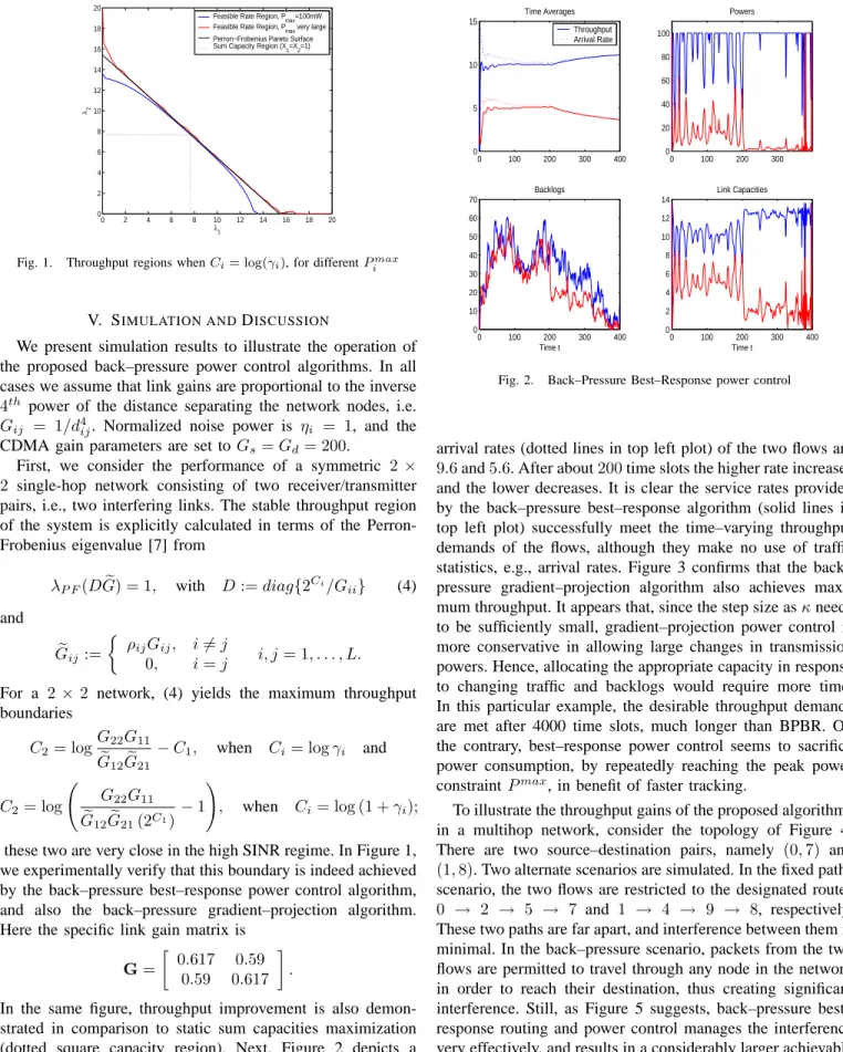
In the same figure, throughput improvement is also demon-strated in comparison to static sum capacities maximization (dotted square capacity region). Next, Figure 2 depicts a sample evolution of powers (with Pmax = 100mW), traf-fic backlogs, instantaneous link capacities and time-averaged throughputs and arrival rates. Initially, the nominal Poisson
0 100 200 300 400 0 5 10 15 Time Averages Throughput Arrival Rate 0 100 200 300 0 20 40 60 80 100 Powers 0 100 200 300 400 0 10 20 30 40 50 60 70 Time t Backlogs 0 100 200 300 400 0 2 4 6 8 10 12 14 Time t Link Capacities
Fig. 2. Back–Pressure Best–Response power control
arrival rates (dotted lines in top left plot) of the two flows are
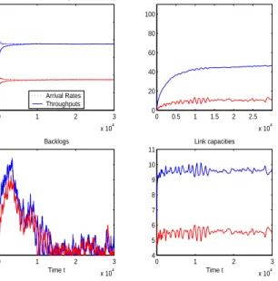
9.6and5.6. After about200time slots the higher rate increases and the lower decreases. It is clear the service rates provided by the back–pressure best–response algorithm (solid lines in top left plot) successfully meet the time–varying throughput demands of the flows, although they make no use of traffic statistics, e.g., arrival rates. Figure 3 confirms that the back– pressure gradient–projection algorithm also achieves maxi-mum throughput. It appears that, since the step size asκneeds to be sufficiently small, gradient–projection power control is more conservative in allowing large changes in transmission powers. Hence, allocating the appropriate capacity in response to changing traffic and backlogs would require more time. In this particular example, the desirable throughput demands are met after 4000 time slots, much longer than BPBR. On the contrary, best–response power control seems to sacrifice power consumption, by repeatedly reaching the peak power constraintPmax, in benefit of faster tracking.
To illustrate the throughput gains of the proposed algorithms in a multihop network, consider the topology of Figure 4. There are two source–destination pairs, namely (0,7) and
(1,8). Two alternate scenarios are simulated. In the fixed paths scenario, the two flows are restricted to the designated routes
0 → 2 → 5 → 7 and 1 → 4 → 9 → 8, respectively. These two paths are far apart, and interference between them is minimal. In the back–pressure scenario, packets from the two flows are permitted to travel through any node in the network in order to reach their destination, thus creating significant interference. Still, as Figure 5 suggests, back–pressure best– response routing and power control manages the interference very effectively, and results in a considerably larger achievable throughput region, which is also the maximum possible. One might argue that the comparison is unfair, due to multiple alternate paths in the latter scenario, however this stands for
0 1 2 3 x 10⁴ 2 4 6 8 10 12 14 Time Averages Arrival Rates Throughputs 0 0.5 1 1.5 2 2.5 x 10⁴ 0 20 40 60 80 100 Powers 0 1 2 3 x 10⁴ 0 100 200 300 400 500 600 700 Time t Backlogs 0 1 2 3 x 10⁴ 4 5 6 7 8 9 10 11 Time t Link capacities
Fig. 3. Back–Pressure Gradient–Projection power control (κ= 0.001)
wired networks. In the wireless case, multiple transmissions generate higher interference making gains in throughput more difficult; hence the comparison makes sense.
In closing, we note that whenever the high SINR assumption is not satisfied, this may be enforced by temporarily shutting down the low SINR links. Also, the present setup did not account for user mobility, or time variations in the wireless channel. These topics are the subject of ongoing and future work. 0 2 3 1 4 5 6 9 7 8
Fig. 4. Multihop network topology
VI. CONCLUSIONS ANDEXTENSIONS
We proposed distributed power control algorithms for wire-less multihop networks, aiming at maximizing the overall network throughput. This is indeed accomplished in the high SINR regime. Joint routing, scheduling and power control decisions are taken in real–time, according to a back–pressure policy. Each node contains a separate queue per destination, and links charge each other a cross–layer interference and backlog related price. Throughput optimal power updates are derived from the solution to a convex optimization problem. The algorithms achieve maximum throughput without knowl-edge of traffic statistics, hence they can dynamically respond to changes in traffic. Simulation results confirm the desired performance. 0 2 4 6 8 10 12 14 16 0 2 4 6 8 10 12 14 16 back−pressure 2 fixed paths
Fig. 5. Throughput improvement due to back-pressure routing
In a companion paper [4], the power control algorithms are modified so that throughput maximization is achieved while also minimizing the required energy expenditure. Furthermore, whenever the arrival rates lie outside the network stable throughput region, flow control is necessary; this situation is also treated in [4].
REFERENCES
[1] T. Alpcan, T. Bas¸ar, R. Srikant and E. Altman, ”CDMA Uplink Power Control as a Noncooperative Game”, Wireless Networks, Kluwer Aca-demic Publishing, Nov. 2002.
[2] M. Chiang, “Balancing Transport and Physical Layers in Wireless Multi-hop Networks: Jointly Optimal Congestion Control and Power Control”, IEEE Journal on Selected Areas in Communications, vol. 23, no. 1, Jan. 2005.
[3] G. Foschini and Z. Miljanic, “A Simple Distributed Autonomous Power Control Algorithm and its Convergence”, IEEE Transactions on Vehicular Technology”, vol. 42, no. 4, pp. 641–646, Nov. 1993.
[4] A. Giannoulis, K. P. Tsoukatos and L. Tassiulas, “Lightweight Cross– layer Control Algorithms for Fairness and Energy Efficiency in CDMA Ad–Hoc Networks”, 4th International Symposium on Modeling and Optimization in Mobile, Ad-hoc and Wireless Networks, WiOpt ’06, Boston (MA), April 3 - 7, 2006.
[5] A. Giannoulis, K. P. Tsoukatos and L. Tassiulas, “Maximum Through-put Back–Pressure Power Control in Multihop Wireless Networks”, in preparation.
[6] J. Huang, R.A. Berry, and M.L. Honig, “A Game Theoretic Analysis of Distributed Power Control for Spread Spectrum Ad Hoc Networks”, in IEEE International Symposium on Information Theory (ISIT’05), Adelaide, Australia, September 2005.
[7] D. O’ Neill, D. Julian, and S. Boyd, “Seeking Foschini’s Genie: Optimal Rates and Powers in Wireless Networks”, IEEE Transactions on Vehicular Technology, 2004.
[8] X. Qiu, and K. Chawla, “On the Perfomance of Adaptive Modulation in Cellular Systems”, IEEE Transactions on Communications, vol. 47, no. 6, Jun. 1999.
[9] C. U. Saraydar, N. B. Mandayam and D. J. Goodman, “Pricing and Power Control in a Multicell Wireless Data Network”, IEEE Journal on Selected Areas in Communications, vol. 19, no. 10, Oct. 2001.
[10] S. Shakkottai and A.L. Stolyar, “Scheduling Algorithms for a Mixture of Real-Time and Non-Real-Time Data in HDR”, in Proceedings of the 17th International Teletraffic Congress - ITC-17, Salvador da Bahia, Brazil, Sep. 2001, pp. 793-804.
[11] C.W. Sung and K.K. Leung, “Opportunistic power control for throughput maximization in mobile cellular systems”, IEEE Proc. ICC, pp. 2954-2958, Paris, France, Jun. 2004.
[12] L. Tassiulas and A. Ephremides, “Stability Properties of Constrained Queueing Systems and Scheduling Policies for Maximum Throughput in Multihop Radio Networks”, IEEE Transactions on Automatic Control, vol.37, no. 12, Dec. 1992.
[13] M. Xiao, N. B. Shroff and E. K. P. Chong, “A Utility Based Power-Control Scheme in Wireless Cellular Systems”, IEEE/ACM Transactions on Networking, vol. 11, no. 2, Apr. 2003.