Boston University
OpenBU http://open.bu.edu
Theses & Dissertations Boston University Theses & Dissertations
2017
Automatic generation of hardware
Tree Classifiers
https://hdl.handle.net/2144/23688 Boston University
Thesis
AUTOMATIC GENERATION OF HARDWARE TREE CLASSIFIERS
by
KIRAN VISHAL THANJAVUR BHAASKAR
B.Eng., Anna University, 2015
Submitted in partial fulfillment of the requirements for the degree of
Master of Science 2017
© 2017 by
KIRAN VISHAL THANJAVUR BHAASKAR All rights reserved
First Reader
Martin C. Herbordt, Ph.D.
Professor of Electrical and Computer Engineering
Second Reader
Wenchao Li, Ph.D.
Assistant Professor of Electrical and Computer Engineering Assistant Professor of Computer Science
Third Reader
Brian Kulis, Ph.D.
Assistant Professor of Electrical and Computer Engineering Assistant Professor of Systems Engineering
“The only way to do great work is to love what you do. If you haven’t found it yet keep looking. Don’t settle. As with all matters of the heart, you’ll know when you find it.”
v
ACKNOWLEDGMENTS
I would like to thank Professor Martin Herbordt, for giving me the opportunity to work with him on this thesis. It has been a great learning experience which wouldn’t have been possible without his guidance and support all the way until the end. I would like to thank the researchers at CAAD Lab and at the Computer Research Lab (PHO340) in Boston University, their insights and extensive research knowledge was very valuable and helped me in reaching the goal of automation for machine learning algorithms on hardware. Assistant Professors Wenchao Li and Brain Kulis have been very honest and made sure my work was well reviewed and acceptable. I would also like to thank Marcia Shaya Louis for helping me through the world of Chisel. Finally, my parents who have been very understanding and making sure I stay calm and prepared through the whole process.
vi
AUTOMATIC GENERATION OF HARDWARE TREE CLASSIFIERS KIRAN VISHAL THANJAVUR BHAASKAR
ABSTRACT
Machine Learning is growing in popularity and spreading across different fields
for various applications. Due to this trend, machine learning algorithms use different hardware platforms and are being experimented to obtain high test accuracy and
throughput. FPGAs are well-suited hardware platform for machine learning because of its re-programmability and lower power consumption. Programming using FPGAs for machine learning algorithms requires substantial engineering time and effort compared to software implementation. We propose a software assisted design flow to program FPGA for machine learning algorithms using our hardware library. The hardware library is highly parameterized and it accommodates Tree Classifiers. As of now, our library consists of the components required to implement decision trees and random forests. The whole automation is wrapped around using a python script which takes you from the first step of having a dataset and design choices to the last step of having a hardware
vii
TABLE OF CONTENTS
ACKNOWLEDGMENTS ... v
ABSTRACT ... vi
TABLE OF CONTENTS ... vii
LIST OF TABLES ... ix
LIST OF FIGURES ... x
LIST OF ABBREVIATIONS ... xii
1. INTRODUCTION ... 1 2. MACHINE LEARNING ... 5 2.1 Decision Trees ... 6 2.2 Random Forests ... 8 3. RELATED WORK ... 10 4. AUTOMATIC GENERATION ... 12 4.1 Training Phase ... 13 4.2 Visualization Phase ... 15
4.3 Hardware Code Generation Phase ... 16
5. HARDWARE IMPLEMENTATION ... 23
5.1 Building Block Library ... 23
viii
5.3 Hardware Implementation of Random Forest ... 25
5.4 Node Memory ... 26
5.5 Node Connection Diagram ... 28
6. RESULTS ... 29
7. FUTURE WORK ... 34
7.1 GUI – Decision Tree ... 34
7.2 GUI – Random Forest ... 35
ix
LIST OF TABLES
Table 1. Results – Datasets and their properties ... 29
Table 2. Results – Software version code accuracy ... 29
Table 3. Results – Decision tree train and test time for CPU ... 30
x
LIST OF FIGURES
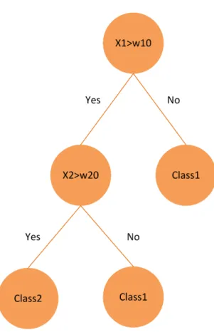
Figure 1. Decision tree ... 6
Figure 2. Random Forest ... 8
Figure 3. Automatic generation of hardware tree classifier ... 12
Figure 4. Training phase of automatic generation ... 13
Figure 5. Sample input dataset ... 14
Figure 6. Visualization phase of automatic generation ... 15
Figure 7. Code - Generalized visualization ... 16
Figure 8. Automatic generation - Hardware generation phase ... 17
Figure 9. Code – Extraction of trained model ... 18
Figure 10. Sample – Node memory entry ... 19
Figure 11. Sample – Generated Verilog and C+++ codes ... 20
Figure 12. Sample – Instantiation of comparators, and population of node memory ... 21
Figure 13. Sample – Functional verification of comparator using C++ emulator ... 22
Figure 14. Hardware implementation – Decision tree ... 24
Figure 15. Hardware implementation – Random forest ... 25
Figure 16. Hardware implementation – Node memory ... 26
Figure 17. Sample – Node memory mapping ... 27
Figure 18. Hardware implementation - Node memory connection to tree comparator .... 28
Figure 19. Results – Visualization of Iris dataset ... 31
Figure 20. Results – Visualization of Breast Cancer dataset ... 32
xi
xii
LIST OF ABBREVIATIONS
AI ... Artificial Intelligence ASIC ... Application Specific Integrated Circuit CPU ... Central Processing Unit FPGA ... Field-Programmable Gate Array GPU ... Graphics Processing Unit GUI ... Graphical User Interface HDL ... Hardware Description Language URL... Uniform Resource Locator FFT ... Fast Fourier Transform
1. INTRODUCTION
Machine learning is the ability to learn without being explicitly programmed [1]. Machine learning does not impose a set of fixed rules and it also involves highly data parallel computation.
CPU can be used for machine learning applications. Although in general, they take a longer time to train and test machine learning algorithms than other hardware platforms. CPU is not well suited for machine learning applications mainly because it is not as parallel as GPUs or FPGAs and also can't handle the data rate needed for efficient testing of data.
GPUs is well suited for machine learning applications due to its parallel architecture. GPUs have high bandwidth memory and thousands of cores to handle the high testing data rates. GPUs also currently have a huge number of machine learning frameworks and software libraries. But GPUs consume huge amounts of power. Also, inter-block
communication and irregular data access slow the performance of GPU.
FPGAs are also well suited for machine learning because they can be programmed to perfectly fit machine learning algorithms. And the power consumed by FPGA is lower than a GPU. FPGAs also have high data transfer rates and can be programmed to parallel process incoming data, which addresses the high testing data rates. Architectures with very deep pipelines can also be designed using FPGAs [15]. The drawback of FPGAs is
2 that they consume a lot of time to program. My goal is to make FPGAs easier to program and implement machine learning algorithms.
In this paper, we propose an automatic generation of tree classifier which can be implemented on an FPGA. The proposed implementation is made of two main components.
• Automatic Generation of Hardware Tree Classifiers.
• Building Block library for machine learning on FPGAs.
Decision tree is a machine learning classifier. The way the decision tree works is very similar to how humans make decisions. Like humans, the final classification of the input is dependent on multiple factors and how we weight them against other options. Decision tree algorithm is very intuitive and efficient in classifying data. The downside to decision tree is that it can often over-fit the data.
Random forest is a special kind of decision tree. The dataset for training is broken into smaller batches of overlapping data. These smaller batches of data are used to train multiple smaller trees. The final classification decision is made by taking a majority vote among the smaller trees. The random forest algorithm is very efficient and eliminates the over-fitting problem. The downside to this algorithm is that it is highly memory intensive when compared to the decision tree. The higher memory requirement is due to the storage of node memory for multiple smaller trees instead of one larger tree.
The Automatic Generation design flow is used to obtain a hardware implementable code for machine learning algorithm. The whole automatic generator is wrapped around in a python script. The python script takes the user from having a dataset and some design choices to the final step of obtaining the hardware descriptive code. The python script on the terminal level poses the user with questions regarding the dataset to be used, the type of tree classifier used and then design choices for the chosen tree classifier. The script then uses this information and trains the desired tree model using the SciKit-Learn[2] machine learning library. At this point, a trained model based on the choices provided and a software version of the model is obtained.
The trained model along with the features and label names from the dataset is parsed through Graphviz [3] visualization Library based generic code. The visualization code provides us with an image of the trained tree, which helps the user get a better
understanding of how the trained tree actually looks like. If the user is not satisfied with the results, the user can run the script again and choose different parameters to obtain the desired tree.
The trained model is then extracted by the script to collect information needed to generate the hardware implementation. The building block library components are used to create the tree and are written using Chisel [4] hardware descriptive code. The parameters used in the Chisel code are updated during compilation by using the information extracted from the trained model. After compilation, the user is provided with a Verilog hardware
4 code which can be burnt on the FPGA and also a C++ emulator version for functional verification.
The building block library is written using a hardware descriptive language called Chisel. The library currently is made of modules, which are required for implementing decision trees and random forests on FPGA.
The library can be used to design and implement either of the two classifier trees. All the components needed for the implementation is highly parameterized and can be used in their default connection. Or the user can use the modules and connect them differently based on the design requirements.
The automatic generation reduces the need to write code for the tree classifier and takes you directly to the hardware implementation stage. For more complex designs the library can be imported and used as per the linking of the user which also significantly reduce the coding time required and acts as a good start point.
2. MACHINE LEARNING
Machine Learning is a type of artificial intelligence (AI). Machine learning allows the computer to learn for itself and it is not explicitly programmed. Machine learning does not impose a fixed set of rules for the computer to follow. Rather it provides the computer with the ability to learn and change when exposed to new data.
In the process of machine learning, the computer searches the input dataset and looks for patterns. Using the seen pattern is updates itself and can detect such patterns in the future. Machine learning algorithms are broadly classified into two categories supervised machine learning and unsupervised machine learning.
Supervised machine learning is more widely compared to unsupervised learning. In supervised learning, the goal is to approximate a mapping function so that an input can be used to predict an output for the given data. Here a set of input variables along with output variables is given to a machine learning algorithm. The machine learning algorithm helps learn the mapping function from the input to the output and produces a trained model.
Supervised machine learning is further grouped into two categories
• Classification
• Regression
Unsupervised machine learning is where there is no output data to map the input data. The algorithm is only provided with input data and no output data. The
6 it learn about the data provided. Unsupervised learning algorithms also learn from the distribution of the data which again helps it learn more about the data.
Unsupervised learning algorithms are also further classified into two categories
• Clustering
• Association
We as part of the thesis will be focusing on two supervised machine learning algorithms. The two algorithms fall under classification subdivision of supervised machine learning.
2.1 Decision Trees
Decision Trees are similar to how humans make decisions. The decision tree consists of multiple nodes. There are two types of nodes namely the non-leaf node and the leaf nodes. The non-leaf nodes are where the decisions are made and have two
children nodes. The children node can be non-leaf node or a leaf node. The non-leaf node uses the input feature value and compares it to the threshold, depending on the decision the data is then passed on to the left or the right node. This process in continued till a leaf node is reached. Leaf nodes are the termination node. The leaf node provides the
classification of input data.
Initially, an input data is provided to the root node. Once the root node makes a decision it passes the data down to the left or right node. The data is then used to make a decision at this level and the data flows to the leaf node by repetition of this process. The leaf node contains information about which class this data belongs to and thereby a final classification result can be achieved.
Each level of the decision tree contributes to the depth of the tree. This brings us to the disadvantage of the decision tree. Even though the decision tree is very intuitive and easy to understand the depth of the tree causes the problem. A decision tree grows in depth and reaches to a point of having all the leaf nodes in the final level. And this introduces the problem of over-fitting and masks the idea of true learning.
8
2.2 Random Forests
The second algorithm is the random forest algorithm. This algorithm is also a type of supervised algorithms and belongs to the classification subdivision. Random forest is a special type of decision tree algorithm which eliminates the over-fitting problem.
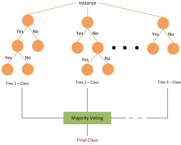
Figure 2. Random Forest
Random forest is machine learning algorithm where multiple smaller decision trees are formed and their results are combined to reach the final classification. Instead of providing the whole training dataset to form a single decision tree, smaller training datasets are formed by extracting chunks of overlapping data from the parent dataset. Using these individual smaller datasets, decision trees are trained. Since smaller
These depths are definitely smaller than what you would get if the same dataset was used to train a single tree. Also, since now these smaller trees are not exposed to the entirety of the training dataset they are more generalized and robust to newer input data.
The process of classification is very similar to that of decision tree with one main difference. In random forests, the same input data is given to all the different decision trees and multiple classification results are obtained. These results are then passed on to a majority voting node which provides the final classification result.
Although the problem of over-fitting was eliminated, we reach a new problem. Since we now have multiple decision trees we have to store all their information which makes random forests more memory intensive.
10
3. RELATED WORK
Machine learning is being used in various applications and scope for machine learning applications are growing enormously. Traditionally, most of these applications are implemented in general purpose CPUs and GPUs.
An example of a machine learning application on a GPU, [5] implements the training and evaluation of decision trees and random forests on a GPU. According to the results, near real-time performance with identical accuracy to the CPU results is obtained.
In recent years there is an increasing trend of using specialized hardware accelerators for machine learning applications to gaining performance and energy efficiency. One such specialized hardware accelerator is ASIC. PuDianNao [6] is a machine learning accelerator implemented in ASIC. This implementation includes seven machine learning algorithms namely k-means, k-nearest neighbors, naive Bayes, support vector machine, linear regression, classification tree and deep neural network. ASIC is highly efficient in terms of power and performance, however, it does not provide flexibility.
Consequently, researchers consider FPGA hardware as an appealing accelerator platform for implementing machine learning algorithms due to its re-programmable property. [7] Implements an axis parallel pipelined architecture for decision tree model. To achieve high throughput in this implementation, the pipeline architecture is
instantiated 8 times thereby processing multiple data streams independently.
Deep Burning [8] is an automatic generator of hardware descriptive code for machine learning algorithms like Multiple Layer Perceptron, Convolutional Neural
Network, Recurrent Neural Network for FPGA-based acceleration. But here the Caffe code is used to generate the HDL and so involves experience in using Caffe deep learning framework.
Intel Deep Learning Interface Accelerator [9] is an integrated hardware and software solution for accelerating Convolutional Neural Network using Caffe framework and accelerating the trained model using FPGA.
FPGA can also be clustered together. FPGAs provide low latency [14] and high bandwidth transceivers. These factors become beneficial for distributed applications and applications that need high data transfer rates. Previous work by M. Herbordt [13] shows a possible application of FPGA clusters for 3D FFTs.
Implementation on FPGAs come with the most benefits in terms of performance, energy efficiency and flexibility. The benefits provided by the above three factors helps set FPGAs apart from the other hardware platforms and gave us enough motivation to pursue an FPGA implementation for machine learning applications.
12
4. AUTOMATIC GENERATION
In this section, the automatic generation of machine learning algorithms for hardware implementation will be explained. The diagram below is the block diagram for the automatic generation design flow.
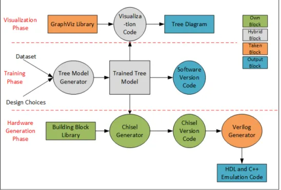
Figure 3. Automatic generation of hardware tree classifier
The block diagram is the design flow which is wrapped around using a python script. The python script is written in a way that takes the user step by step through the whole design flow till the hardware descriptive code is achieved. The python code poses simple questions to the user and takes the inputs from the user. These inputs are then provided to the respective blocks to achieve their goal.
The automatic generation is divided into three phases.
• Visualization Phase
• Hardware Code Generation Phase
4.1 Training Phase
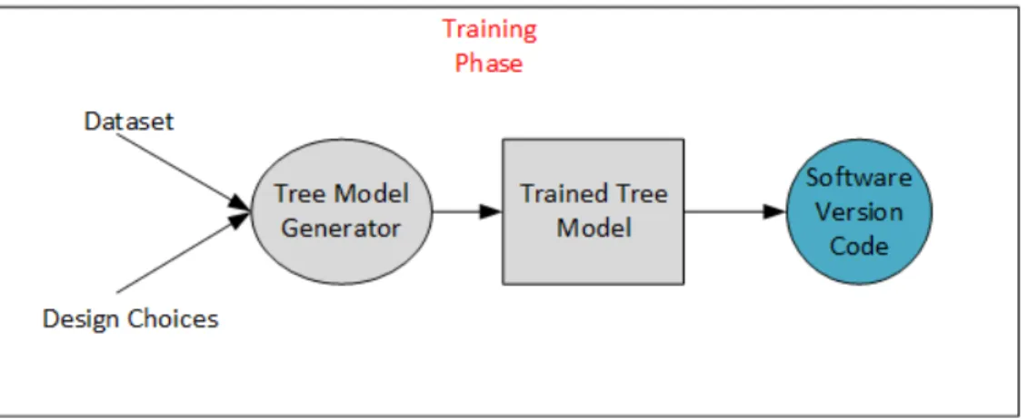
Figure 4. Training phase of automatic generation
Training phase takes the user from having an input dataset and design choices to obtaining a trained machine learning software model. The python script once started asks the user to provide an input dataset for training any machine learning model. The
provided dataset has to be of a particular format. All the features have to be listed first in form of columns followed by the labels in the last column. Then the user is asked to pick one of the two machine learning algorithms that are currently available. Once the user selects a particular algorithm, the user is then asked to provide the different design choices to train the model.
14
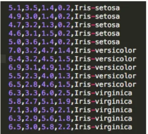
Figure 5. Sample input dataset
The above snippet shows the features listed in the first four columns followed by the labels listed in the last columns. A similar dataset of user choice along with the user design choices are then provided to the Python Scikit-Learn Library.
Scikit-Learn is a machine learning library written in python. It is an open source library which consists of multiple machine learning algorithms. The tree model generator has two versions of codes written using the scikit-learn library. One version is written to accept values if the decision tree algorithms are chosen and the other is for random forests. Using these two versions and the user inputs, an appropriate machine learning model is trained.
The trained model is also the software version for the machine learning algorithm formed by using the user choices. This can be run on a CPU to get the accuracy results which then can be used to compare with the FPGA accuracy.
4.2 Visualization Phase
The next phase in the automatic generation is the visualization phase. This phase is mainly meant to provide the user with a visual representation of how the decision tree or random forest will look like.
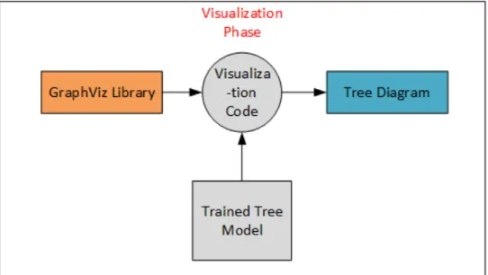
Figure 6. Visualization phase of automatic generation
In the above block diagram, the trained tree model is connected to the
visualization code block. The visualization code block has a generic code written which is expecting feature names, label names and the trained model to produce a visualization. This code was written using the GraphViz Library.
GraphViz library is an open source library which is well integrated with the python scikit-learn library. The main goal of the GraphViz Library is to envision connections. So using the information in the trained model, feature names and the label names passed to it from the previous step, it produces a plot which shows the various connections between the non-leaf and leaf nodes. This step is important for a new user
16 because it gives them a better understand of how the connections are formed in the tree, what feature was used as the split point in a particular node and also where the final classification is achieved.
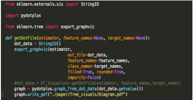
Figure 7. Code - Generalized visualization
The above diagram shows the code snippet of the visualization code. Here the “feature_names” is the list of feature names provided through the python code and similarly the “target_names” are the list of labels from the dataset initially provided.
4.3 Hardware Code Generation Phase
The last phase is called the hardware code generation phase and it is also the most crucial phase for obtaining the final implementation code.
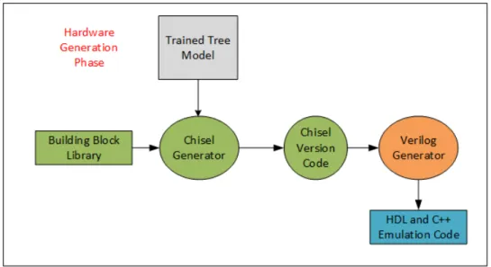
Figure 8. Automatic generation - Hardware generation phase
This phase also using the trained tree model from the training phase. The chisel generator is connected to both the trained tree model as well as the building block library. Building block library will be explained in detail later in section x.
Chisel is a hardware descriptive language written in Scala. Chisel was developed by University of California, Berkeley. Chisel is highly parameterized and on compilation can provide a synthesizable Verilog code. The added advantage of using Chisel is that it can provide a C++ emulator version, which can be used for functional verification of the different block before moving on to the hardware implementation stage.
In this phase, the trained tree model is extracted to produce a text file which contains information to form the node memory and connections between the different comparators in hardware. The building block library contains the required components to create the tree. The modules needed for the requirement tree implementation is available in the chisel generator and it is parameterized.
18 The text file is then accessed by the chisel generator and updates its parameters based on what the text file contains. The chisel code in then compiled using the python script to produce both the Verilog version and the C++ emulator version.
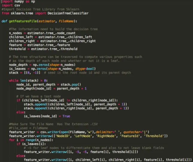
Figure 9. Code – Extraction of trained model
The above code snippet shows the extraction code to obtain the connection and node information from the trained tree model. This is then written to the text file.
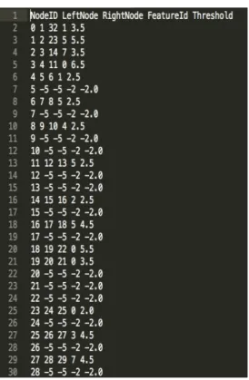
Figure 10. Sample – Node memory entry
The above figure shows a sample extracted text file. The values in the text file are used to populate the node memory. Also, based on entries in the text file an optimal number of comparators is chosen for implementation.
20
Figure 11. Sample – Generated Verilog and C+++ codes
The figure above shows a sample “build folder”. The chisel code on compilation produces different files and these files are stored in the build folder. It is seen from the image that both the “.v” and the “.cpp” files are generated.
Figure 12. Sample – Instantiation of comparators, and population of node memory
The above screen capture is the result of chisel code compilation. The image shows the number of comparators was instantiated, node memory being stored and also information about the total number of nodes, non-leaf nodes, and the leaf nodes.
22
Figure 13. Sample – Functional verification of comparator using C++ emulator
The above screen capture shows the result of running the “.cpp” code. Here it shows how a comparator’s function can be verified by running a test bench. If a test is successful, you get a pass this helps you determine if you achieved the desired
5. HARDWARE IMPLEMENTATION 5.1 Building Block Library
Hardware description for the different modules required to implement the machine learning algorithms are written in chisel. These modules combined to form the building block library. The building block library currently consists of components that are required for decision trees and random forests namely: Register file, comparators, control unit, node memory and majority voting unit. These modules are written from scratch using parameter names which use machine learning terminologies. This makes the chisel code more understandable for machine learning people and easier to alter particular parameters as required.
There are two different ways of using the Building Block Library. The first way is using the automatic generation, the required modules for the selected machine learning algorithms are instantiated and parameters are updated accordingly. The second way is to use it purely as a library, the library can be imported into any user design. The user can just use the ready made blocks or alter the blocks to create more complex architecture, definitely reducing the time consumed since the user is not writing from scratch.
24
5.2 Hardware Implementation of Decision Tree
Figure 14. Hardware implementation – Decision tree
The above block diagram shows current hardware implementation of decision tree algorithm. The control unit is connected to an input queue and an output queue. The input queue provides the input data to be classified and the output queue holds the
corresponding classification result.
The control unit is also connected to two other blocks i.e. the node memory and the tree comparator block. The node memory contains all the information needed to compare the input feature to threshold and pass on the decision. The tree comparator block on the other end has the actual comparator blocks needed to achieve the
fed into the output queue. The node memory and the way it is connected to the tree comparator block will be explained in detail in section x.
5.3 Hardware Implementation of Random Forest
Figure 15. Hardware implementation – Random forest
The hardware implementation of random forests consists of multiple decision tree blocks. Each smaller decision tree is mapped into its own hardware block. The blocks
26 each produce an output for the same output. The output from all the different blocks are then routed into the majority voting block. There based on the majoring classification, a final classification result is computed and stored in the final output queue.
The hardware implementation of random forests is done in the above-shown way to make it more intuitive for new user and users who are new to hardware descriptive coding. This architecture can be altered by connecting the blocks in the building block library as per the user design requirements.
5.4 Node Memory
Node memory consist of the different components needs to form the tree. Each entry in the node memory consists of 5 fields each of 32bit width. The five fields are current node number, left node number, right node number, split feature and the threshold value.
Figure 17. Sample – Node memory mapping
The current node number gives information about which node the computation is currently at. The corresponding threshold value is loaded into the comparator. Then the split feature is used to select the particular feature from the input data which will be used in the comparator. Once this comparison is done, depending on the decision the left node number or right node number is selected. And the node memory entry for that selected node number is retrieved. The leaf node has a threshold of -2 which helps to notify that a leaf node has been reached and the classification result can be obtained.
28
5.5 Node Connection Diagram
Node memory is mapped to the tree comparator block were the actual comparisons are performed.
Figure 18. Hardware implementation - Node memory connection to tree comparator
In the above diagram, one of the comparator nodes is zoomed in to show how the comparator is mapped with the node memory. The current node number is used to retrieve the required information for performing the comparisons. During the non-leaf steps the left or right node number from the previous decision becomes the current node number and the corresponding entry is retrieved. The process of retrieving and loading continues till a leaf node is reached. And the result is sent back to the control unit and stored in the output queue.
6. RESULTS
Three different datasets were used and implemented using the automatic generation of hardware tree classifiers.
Dataset Name Number of data
points
Number of Features Number of Classes
Iris Dataset [10] 150 4 3
Breast Cancer [11] 699 9 2
Digits [12] 1797 64 10
Table 1. Results – Datasets and their properties
Using the training phase these datasets were passed into the automatic generation design and the software versions were obtained.
Dataset Name Number of nodes CPU Accuracy
Iris Dataset 17 94%
Breast Cancer 63 97%
Digits 277 86%
Table 2. Results – Software version code accuracy
The trained model is then extracted to obtain the node information to form the node memory. Also, the depth information for the decision tree and a random forest is obtained.
30
Dataset Name Train time Test time(20 % of dataset)
Digits 16ms 4ms
Table 3. Results – Decision tree train and test time for CPU
The table 3 gives us an idea about the CPU performance for the Digits dataset. For the test data, 20% of the original dataset is reserved and the remaining 80% of the data is used for training the decision tree model.
Dataset Name Number of nodes Decision Tree
Depth Random Forest Depth - 3 Trees Iris Dataset 17 6 4 Breast Cancer 63 10 6 Digits 277 13 7
Table 4. Results – Tree classifier depths for different datasets
Next, the trained model along with the visualization tool are used to produce the visual representation of the trained decision tree models. The two diagrams shown below, are the visualizations obtained for the iris and the breast cancer dataset. The visualization provides nodes and information about the connection between the nodes. Each node also contains information about which feature was used as the split feature, the threshold value, the class label and the number of samples at that node.
32
After seeing the visualization, the user can decide to go ahead with the next step or go back and provide the script with new design choices.
Next, the extracted information from the trained model is used to update the parameters of the chisel code. On compilation, this then produces the final step of obtaining the Verilog hardware descriptive code and the C++ emulator code.
34
7. FUTURE WORK
As of now, the automatic generation design flow is using a terminal level python script to communicate to the user. The next step to make it more interactive would be to develop a GUI and also host the website so it can be accessed remotely.
Adding more machine learning algorithms and their respective building block components to the library. Also, Open Sourcing the building block library so that more algorithms and different implementations of existing algorithms can be contributed.
7.1 GUI – Decision Tree
The above diagram shows a sample visualization of how the decision tree GUI might look like. The user can upload a dataset using the choose file option. Also, provide the different design choices for the decision tree algorithm. Visualize button to obtain the visual representation of the decision tree. Lastly, a compile button which on pressing will produce the Verilog and the C++ codes for the trained model. This can then be
synthesized and burnt on the FPGA board.
7.2 GUI – Random Forest
36 The main difference between the two GUIs is that the random forest version comes with an extra design choice field. This field “N_trees” lets the user decide the number of smaller decision tree need for the implementation.
8. REFERENCES
[1] Munoz, Andres. “Machine Learning and Optimization.” URL: https://www. cims. nyu. edu/~ munoz/files/ml_optimization.pdf [accessed 2016-03-02][WebCite Cache ID 6fiLfZvnG] (2014).
[2] Pedregosa, F. et al., “Scikit-learn: Machine learning in Python.” Journal of Machine
Learning Research, 12, pp. 2825-2830, 2011.
[3] Gansner, E.R. and S.C. North, “An open graph visualization system and its
applications to software engineering.” Journal of Software: Practice and Experience,
30(11), pp. 1203–1233, 2000.
[4] Bachrach, J., H. Vo, B. Richards, Y. Lee, A. Waterman, R. Avizienis, J. Wawrzynek, and K. Asanovic. “Chisel: Constructing hardware in a Scala embedded language.” In
Proceedings of the 49th Annual Design Automation Conference, DAC ’12. ACM, 2012. [5] Sharp, T. “Implementing decision trees and forests on a GPU.” In Forsyth D., Torr P.,
Zisserman A. (eds.),Computer Vision – ECCV 2008. 10th European Conference on
Computer Vision. Volume 5305 of Lecture Notes in Computer Science. Springer-Verlag:
Berlin Heidelberg, 2008.
[6] Liu, D., et al. “PuDianNao: A polyvalent machine learning accelerator.” ACM
SIGARCH Computer Architecture News – ASPLOS’15, 43(1), pp. 369–381, 2015. [7] Saqib, Fareena, et al. “Pipelined decision tree classification accelerator
implementation in FPGA (DT-CAIF).” IEEE Transactions on Computers, 64(1), 280–
38 [8] Wang, Ying, et al. “Deepburning: Automatic generation of FPGA-based learning
accelerators for the neural network family.” In DAC ’16: Proceedings of the 53rd Annual
Design Automation Conference, article 110. ACM/EDAC/IEEE. IEEE, 2016. [9] Intel DLIA, URL : [https://www-ssl.intel.com/content/www/us/en/design/data-centers/server-accelerators/canyon-vista/intel-deep-learning-inference-accelerator.html] [accessed 2017-04-15]
[10] Lichman, M. (2013). UCI Machine Learning Repository
[http://archive.ics.uci.edu/ml/iris}. Irvine, CA: University of California, School of Information and Computer Science.
[11] Lichman, M. (2013). UCI Machine Learning Repository
[http://archive.ics.uci.edu/ml/Breast+Cancer+Wisconsin+(Diagnostic)}. Irvine, CA: University of California, School of Information and Computer Science.
[12] Lichman, M. (2013). UCI Machine Learning Repository
[http://archive.ics.uci.edu/ml/datasets/Pen-Based+Recognition+of+Handwritten+Digits]. Irvine, CA: University of California, School of Information and Computer Science [13] Sheng, Jiayi, et al. "Design of 3D FFTs with FPGA clusters." High Performance Extreme Computing Conference (HPEC), 2014 IEEE. IEEE, 2014.
[14] Sheng, Jiayi, Chen Yang, and M. Herbordt. "Towards Low-Latency Communication on FPGA Clusters with 3D FFT Case Study." Proc. Highly Efficient and Reconfigurable Technologies (2015).
[15] Sanaullah, Ahmed, Arash Khoshparvar, and Martin C. Herbordt.
"FPGA-Accelerated Particle-Grid Mapping." Field-Programmable Custom Computing Machines (FCCM), 2016 IEEE 24th Annual International Symposium on. IEEE, 2016.
40