High-performance computing with PetaBricks and Julia

(1)

High-performance Computing with

PetaBricks and Julia

by

Yee Lok Wong

B.S., Duke University (2006)

MASSACHUSETTS INSTITUTE OF TECHN0LOGY

SEP

0 2 2011

L I

BRA R I ES

Submitted to the Department of Mathematics

in partial fulfillment of the requirements for the degree of

Doctor of Philosophy

at the

MASSACHUSETTS INSTITUTE OF TECHNOLOGY

Yee Lok Wong, 2011. All rights reserved.

The author hereby grants to MIT permission to reproduce and to

distribute publicly paper and electronic copies of this thesis document

in whole or in part in any medium now known or hereafter created.

A uth or ... ... ...

Department of Mathematics

A

April 28, 2011

C ertified by ... ... .. . ...

Alan Edelman

Professor of Applied Mathematics

Thesis Supervisor

Accepted by

Michel Goemans

(2)

(3)

High-performance Computing with

PetaBricks and Julia

by

Yee Lok Wong

Submitted to the Department of Mathematics on April 28, 2011, in partial fulfillment of the

requirements for the degree of Doctor of Philosophy

Abstract

We present two recent parallel programming languages, PetaBricks and Julia, and demonstrate how we can use these two languages to re-examine classic numerical algorithms in new approaches for high-performance computing.

PetaBricks is an implicitly parallel language that allows programmers to naturally express algorithmic choice explicitly at the language level. The PetaBricks compiler and autotuner is not only able to compose a complex program using fine-grained al-gorithmic choices but also find the right choice for many other parameters including data distribution, parallelization and blocking. We re-examine classic numerical algo-rithms with PetaBricks, and show that the PetaBricks autotuner produces nontrivial optimal algorithms that are difficult to reproduce otherwise. We also introduce the notion of variable accuracy algorithms, in which accuracy measures and requirements are supplied by the programmer and incorporated by the PetaBricks compiler and autotuner in the search of optimal algorithms. We demonstrate the accuracy/perfor-mance trade-offs by benchmark problems, and show how nontrivial algorithmic choice can change with different user accuracy requirements.

Julia is a new high-level programming language that aims at achieving perfor-mance comparable to traditional compiled languages, while remaining easy to pro-gram and offering flexible parallelism without extensive effort. We describe a problem in large-scale terrain data analysis which motivates the use of Julia. We perform clas-sical filtering techniques to study the terrain profiles and propose a measure based on Singular Value Decomposition (SVD) to quantify terrain surface roughness. We then give a brief tutorial of Julia and present results of our serial blocked SVD algorithm implementation in Julia. We also describe the parallel implementation of our SVD algorithm and discuss how flexible parallelism can be further explored using Julia.

Thesis Supervisor: Alan Edelman Title: Professor of Applied Mathematics

(4)

(5)

Acknowledgements

Throughout my graduate studies, I have been very fortunate to have met many won-derful people. Without their kind support and help, this thesis would not have been possible.

First and foremost, I would like to thank my advisor Alan Edelman for intro-ducing me to the world of high-performance computing. His enthusiasm, energy and creativity in approaching problems was a constant source of motivation. I am very grateful also for his academic and moral support throughout my time in MIT, and particularly during some of my most difficult time here.

I would also like to express my gratitude to Saman Amarasinghe, who has provided

me with great advice for the PetaBricks project. Thanks goes to the other thesis committee member Gilbert Strang, who offered helpful suggestions for this thesis work.

Special thanks goes to the PetaBricks team, especially Jason Ansel and Cy Chan for the collaboration and inspiring conversations about the PetaBricks project. The Julia team has also been extremely helpful for my work. I owe a special thanks to Jeff Bezanson for implementing a lot of our ideas in Julia in addition to his already long list of tasks. I would also like to thank Martin Bazant, Chris Rycroft and Ken Kamrin for their help and guidance for my early work in MIT.

On the non-academic side, I am extremely grateful to my friends in and outside of MIT. Siu-Chung Yau has provided strong support by his humiliating remarks over our countless phone conversations and by his constant reminder of what my "greatest achievement" is. He also provided motivation by showing by example how bad things could have gone if I had pushed my work and thesis writing to the very last minute. Chloe Kung has been a great friend, with whom I could always have a good laugh and not worry about the stress of work back at school. She also made sure I got real food by going around eating with me every time I went home for Christmas. Annalisa Pawlosky is the most supportive person in MIT, and she believed in my ability probably more than I do myself. She was always there when I needed a friend

(6)

to talk to, and I will never forget the many stories that she has shared with me. Throughout my five years in MIT, the Warehouse graduate dorm has been my home. I would like to extend my heartfelt gratitude to my previous and current housemasters, Lori and Steve Lerman, Anne Carney and John Ochsendorf, for making the Warehouse such a comfortable and warm home for my graduate school life. I must also thank the members of the Warehouse dorm government, especially Allen Hsu, for being great friends throughout these years. I would also like to thank my friends in my second home a.k.a. the Math Department, Linan Chen, Lu Wang, Carol Xia Hua, Ramis Movassagh and Jiawei Chiu, for the inspiring conversations and great times we had in our office.

I must also thank friends of mine outside of MIT who have continued to be a part

of my life: Wai Yip Kong, Leo Lam, Samuel Ng, Siyin Tan, Tina Chang, Edward Chan, Gina Gu, Henry Lam, Jacky Chang, LeVan Nguyen, Nozomi Yamaki and Hiroaki Fukada.

Finally and most importantly, I thank my brother and parents for their continuous support and encouragement since I came to the States for my undergraduate studies nine years ago. The phone conversations with my parents have been a refreshing source of comfort, because talking to my parents was one of the very limited times when I felt smart since I came to MIT. Since the end of my second year here in

MIT, my mom has been asking me what I actually do in school without classes and exams, and my answers never seemed to really convince her that I was indeed doing something. Fortunately, I can now give her a better answer: I wrote this thing called a PhD thesis.

(7)

A.3 k-means clustering . . . . 141 A.3.1 newclusterlocation.pbec . . . . 141 A.3.2 assignclusters.pbec . . . . 143 A.3.3 kmeans.pbec . . . . 144 A.4 Preconditioning . . . . 150 A.4.1 poissionprecond.pbec . . . . 150 B Matlab Code 155 B.1 rmbump.m ... ... 155 B.2 filternoise.m ... ... 157 B.3 gaussfilter.m ... ... 158 B.4 roughness.m . . . . 159 C Julia Code 161 C.1 randmatrixtest.j . . . . 161 C.2 roughness.j. . . . . 161

(11)

List of Figures

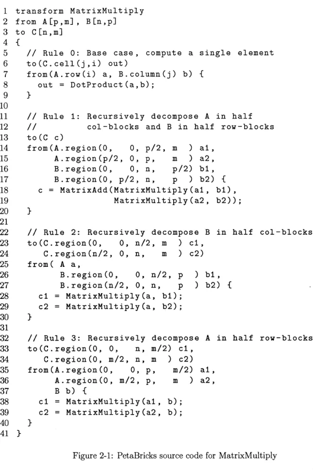
2-1 PetaBricks source code for MatrixMultiply . . . . 49

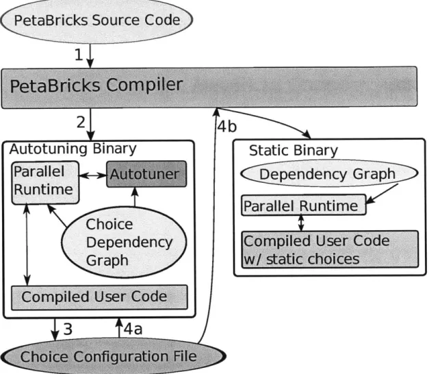
2-2 Interactions between the compiler and output binaries. First, the com-piler reads the source code and generates an autotuning binary (Steps 1 and 2). Next (Step 3), autotuning is run to generate a choice config-uration file. Finally, either the autotuning binary is used with the configuration file (Step 4a), or the configuration file is fed back into a new run of the compiler to generate a statically chosen binary (Step 4b). 50 2-3 PetaBricks source code for CumulativeSum. A simple example used to demonstrate the compilation process. The output element Bk is the sum of the input elements Ao, ... , Ak. . . . . . . . . . . . . . . . . . 51

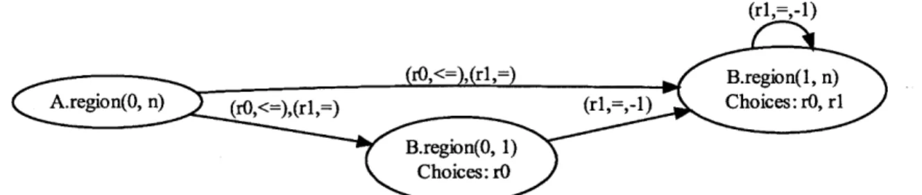
2-4 Choice dependency gmph for CumulativeSum (in Figure 2-3). Arrows point the opposite direction of dependency (the direction data flows). Edges are annotated with rules and directions, offsets of 0 are not shown. 51 2-5 Pseudo code for symmetric eigenproblem. Input T is tridigonal . . . . 51

2-6 Performance for Eigenproblem on 8 cores. "Cutoff 25" corresponds to the hard-coded hybrid algorithm found in LAPACK. . . . . 52

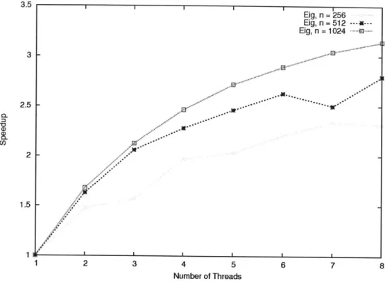
2-7 Parallel scalability for eigenproblem: Speedup as more worker threads are added. Run on an 8-way (2 processor 4 core) x86 64 Intel Xeon System . . . . . 53

2-8 Simple Matlab implementation of right-looking LU . . . . 53

2-9 Pseudo code for LU Factorization. Input A is n x n . . . . 54

(12)

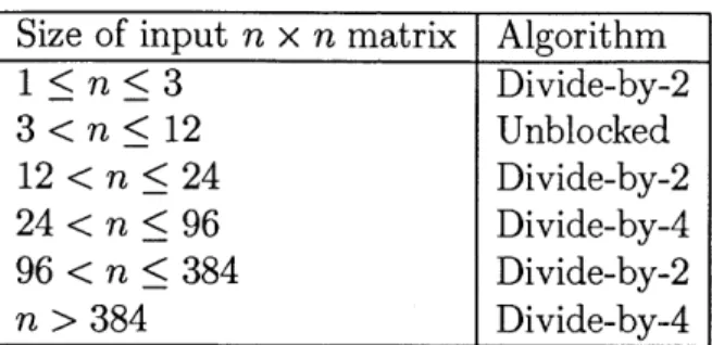
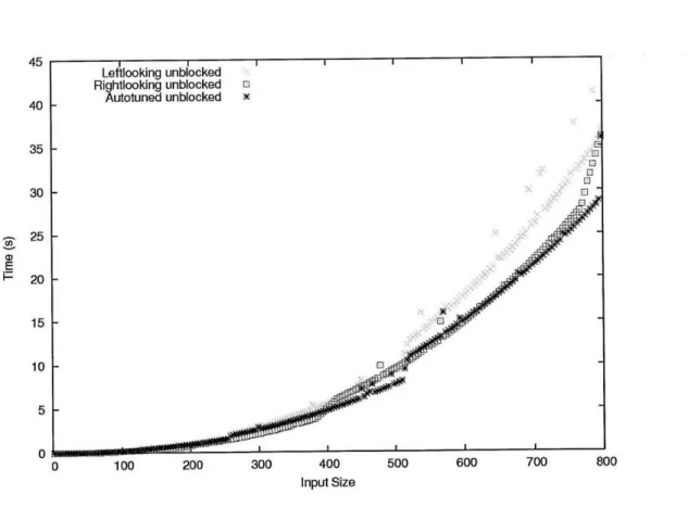
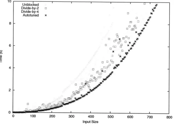
2-11 Performance for LU Factorization on 8 cores. "Unblocked" uses the autotuned unblocked transform from Figure 2-10. . . . . 55

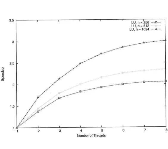
2-12 Parallel scalability for LU Factorization: Speedup as more worker threads are added. Run on an 8-way (2 processor 4 core) x86 64 Intel Xeon System . . . . 56

3-1 Pseudocode for variable accuracy kmeans illustrating the new variable

accuracy language extension. . . . . 76 3-2 Possible algorithmic choices with optimal set designated by squares

(both hollow and solid). The choices designated by solid squares are the ones remembered by the PetaBricks compiler, being the fastest algorithms better than each accuracy cutoff line. . . . . 77

3-3 Pseudo code for k-means clustering . . . . 77

3-4 k-means clustering: Speedups for each accuracy level and input size, compared to the highest accuracy level for each benchmark. Run on an 8-way (2 x 4-core Xeon X5460) system. . . . . 78

3-5 Pseudo code for Preconditioner . . . . 78

3-6 Preconditioning: Speedups for each accuracy level and input size,

com-pared to the highest accuracy level for the Poisson operator A. Run on an 8-way (2 x 4-core Xeon X5460) system. . . . . 79

4-1 Terrain visualization with downsampled data . . . . 84 4-2 Track 1 (left) and Track 2 (right) plooted on the xy-plane . . . . 85

4-3 Terrain Profile with downsampled data (6200 data points are plotted in this figure) . . . . 86

4-4 Vertical lines in red indicate the positions of bumps using the LoG filter with k = 288 . . . . 87

4-5 Top: Terrain Profile with bumps removed. Bottom: Bumps isolated . 94 4-6 Top: Noisy terrain profile. Bottom: Smoothed data . . . . 95

(13)

4-7 Top:

Q-Q

plot of noise, compared with Standard Normal. Bottom: Histogram of noise, and plot of Normal Distribution with the same mean and variance . . . . 96

4-8 Top: Raw terrain profile (Track 2). Bottom: Filtered data . . . . 97

4-9 Top:

Q-Q

plot of noise, compared with Standard Normal. Bottom: Histogram of noise, and plot of Normal Distribution with the same mean and variance . . . . 98

4-10 Top: Noisy terrain profile. Bottom: Smoothed data by SVD . . . . . 99

4-11 Top: dfi of a noisy segment of terrain. Bottom: df2 of a smooth segment 100

5-1 Julia example code . . . . 106 5-2 Parallel scalability for Julia example program: Speedup as more

pro-cesses are added. ... ... 107 5-3 k-th step of Blocked Bidiagonalization. Input A is n x n . . . . 111

(14)

(15)

List of Tables

2.1 Algorithm selection for autotuned unblocked LU . . . . 45 2.2 Algorithm selection for autotuned LU . . . . 46

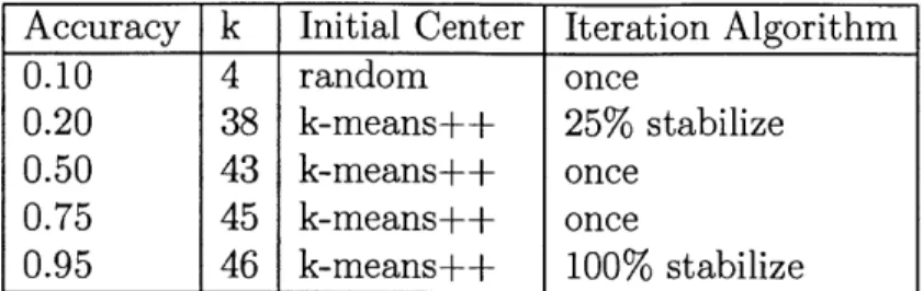
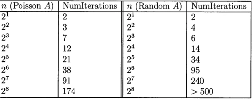
3.1 Algorithm selection and initial k value results for autotuned k-means benchmark for various accuracy levels with n = 2048 and ksource = 45 68 3.2 Values of NumIterations for autotuned preconditioning benchmark

for accuracy level 2 and various size of the n x n input A . . . . 72 3.3 Algorithm selection for autotuned preconditoining benchmark,

accu-racy level = 2 and input A is the Poisson operator . . . . 73

4.1 Statistics of noise for both tracks . . . . 89

4.2 First 5 singular values of dfi (noisy) and df2 (smooth) . . . . 92

4.3 p of the same segment with different level of noise. p gets closer to 1 as the data gets smoother. . . . . 92

(16)

(17)

Chapter 1

Introduction

1.1

Background and Motivation

High-performance computing has become ubiquitous in scientific research and become more and more common even in everyday lives. Many laptops now have multicore processors and smartphones with dual-core processors have entered the market. Per-formance growth for single processors has approached its limit, but Moore's law still predicts that the number of transistors on a chip will double about every two years, and the physical limits would not be reached until the earliest in the year 2020 accord-ing to Intel [1, 71]. With the doublaccord-ing of chip density every 2 years and clock speed not catching up with this growth rate, exposing and managing parallelism between multiple processors by software is the key to getting further performance gain.

One major aspect of parallel computing is to identify enough paralleism. The well-known Amdahl's law [3] states that if f is the fraction of work done sequentially, and (1 -

f)

_{is the fraction parallelizable with n processors with no scheduling overhead,}

the speedup is given by

1

Speedup(f,n) -

f

+ 1

1 (1.1)

(18)

Even if the parallel part speeds up perfectly, parallel performance is still limited by the sequential component. In practice, parallelism involves overhead such as com-municating data, synchronization and managing different threads. A good parallel implementation also needs to take care of locality and dependencies of data, load balancing, granularity, race conditions and synchronization issues.

Historically, the first standardized library for high-performance computing sys-tems was the Message Passing Interface (MPI), which allows the programmer to have control over every detail. Each message passing call has to be individually written, addressed, sent and received. Some of the other early parallel programming standards include High Performance Fortran (HPF) and OpenMP. Following the evolution of hardware, there has been an emergence of different programming languages and li-braries.

However, designing and implementing parallel programs with good performance is still nontrivial despite decades of research and advances in both software and hard-ware. One major challenge is that the choice of algorithms depends not only on the problem size, but becomes more complicated with factors such as different data

distribution, underlying architecture, and number of processors available. In terms of design, it is often not obvious how to choose the optimal algorithms for a specific problem. Complexity analysis gives an idea of how well algorithms perform asymptot-ically, but it gets more complicated when parallelism is involved. Take the symmetric eigenproblem as an example, the common serial algorithms all have 0(n3₎_complexity

to find all eigenvalues and eigenvectors, so it is difficult to find the right composition and cutoffs for an optimal hybrid algorithm in parallel. Asymptotically optimal al-gorithms, called cache-oblivious algorithms [42], are designed to achieve optimality without depending on hardware parameters such as cache size and cache-line length. Cache-oblivious algorithms use the ideal-cache model, but in practice memory system behavior is much more complicated. In addition, even when an optimal algorithm is implemented for a specific configuration, completely different algorithms may provide the best performance for various architectures, available computing resources and in-put data. With the advent of multiple processors, architectures are changing at a fast

(19)

rate. Implementing algorithms that can perform well for generations of architecture has become increasingly important.

Another challenge is the flexibility of parallelism available with the current pro-gramming languages. Parallel propro-gramming introduces complications not present in serial programming, such as keeping track of which processor data is stored on, sending and receiving data while minimizing communication and distributing com-putation among processors. Currently existing languages and API with low-level parallel constructs such as MPI, OpenMP and OpenCL give users full control over the parallelziation process. However, it can be difficult to program since communica-tion is performed by explicitly managing the send and receive operacommunica-tions in the code. Messages and operations on each thread must also be explicitly crafted. On the other end of the spectrum, there are high-level programming languages such as Matlab's parallel computing toolbox, pMatlab [58] and Star-P [21], which allow higher level parallel data structures and functions. Serial programs can be transformed to have parallel functionality with minor modifications, so parallelism is almost "automatic". The trade-off for drastically reducing the difficulty of programming parallel machines is the lack of control of parallelsim. A parallel computing environment, which offers the right level of abstraction and maintains a good balance between parallelization

details and productivity of program development and debugging, is still lacking. In this thesis, we present two recent parallel programming languages, PetaBricks

[6] and Julia [12], and demonstrate how these two languages address some of the

dif-ficulties of high-performance computing. Using PetaBricks and Julia, we re-examine some classic numerical algorithms in new approaches for high-performance

comput-ing.

PetaBricks is a new implicitly parallel language and compiler where having

mul-tiple implementations of mulmul-tiple algorithms to solve a problem is the natural way of programming. Algorithmic choice is made to be a first class construct of the language, such that it can be expressed explicitly at the language level. The PetaBricks com-piler autotunes programs by making both fine-grained as well as algorithmic choices. Choices also include different automatic parallelization techniques, data distributions,

(20)

algorithmic parameters, transformations, blocking and accuracy requirement. A num-ber of empirical autotuning frameworks have been developed for building efficient, portable libraries in specific domains. PHiPAC [13] is an autotuning system for dense matrix multiply, generating portable C code and search scripts to tune for specific systems. ATLAS [88, 89] utilizes empirical autotuning to produce a cache-contained matrix multiply, which is then used in larger matrix computations in BLAS and LA-PACK. FFTW [40, 41] uses empirical autotuning to combine solvers for FFTs. Other autotuning systems include SPIRAL [76] for digital signal processing, SPARSITY [55] for sparse matrix computations, UHFFT [2] for FFT on multicore systems, OSKI [87] for sparse matrix kernels, and autotuning frameworks for optimizing sequential [62, 63] and parallel [73] sorting algorithms. To the best of our knowledge, PetaBricks is the first language that enables programmers to express algorithmic choice at the language level and provides autotuned optimized programs that are scalable and portable in general purpose applications.

Julia is a new high-level programming language that aims at filling the gap

be-tween traditional compiled langauges and dynamic languages by providing a program-ming tool that is easy to use while not sacrificing performance. The Julia project is an ongoing project based at MIT. One of the main goals of the project is to provide flexible parallelism without extensive effort. For example, can the number of pro-cessors used not be fixed by the user, but scale up or down depending on the work waiting? This will become increasingly important when a cloud API is ready for Julia and an external cloud provider is used. How can we minimize unnecessary idle time of threads? What is the right level of abstraction, such that the user will not lose too much control of the parallelism while still being able to program without the need to specify every piece of detail? The Julia project is working to create a cloud friendly environment such that the Julia language is fast and general, easy to use, open source and readily available.

(21)

1.2

Scope and Outline

The rest of this thesis proceeds as follows:

In chapter 2, we introduce the PetaBricks language and describe the implemen-tation of the compiler and autotuning system. The PetaBricks compiler and auto-tuner is not only able to compose a complex program using fine-grained algorithmic choices but also find the right choice for many other parameters including data dis-tribution, parallelization and blocking. We re-examine classic numerical algorithms with PetaBricks, and present experimental results to show that the PetaBricks auto-tuner produces nontrivial optimal algorithms. Specifically, we give a review of classic algorithms used to solve the symmetric eigenvalue problem and LU Factorization. We then show that the optimal PetaBricks algorithm composition for the symmetric eigenvalue problem is different from the one used in LAPACK. We also demonstrate the speedup of LU Factorization implemented using our autotuned nontrivial varaible blocking algorithm over conventional fixed recursive blocking strategies.

We continue with PetaBricks in Chapter 3 by introducing the notion of variable ac-curacy. We present the programming model with PetaBricks where trade-offs between time and accuracy are exposed at the language level to the compiler. We describe the language extensions in PetaBricks to support variable accuracy, and outline how the PetaBricks compiler automatically searches the space of algorithms and param-eters (optimal frontier) to construct an optimized algorithm for each accuracy level required. We demonstrate the accuracy/performance trade-offs by two examples, k-means clustering and preconditioned conjugate gradient. With our experimental results, we show how nontrivial algorithmic choice can change with different accuracy measure and requirements. In particular, we show how k-means clustering can be solved without specifying the number of clusters k, and show that the optimal k can be determined accurately with PetaBricks using relevant training data. We also show that the optimal choice of preconditioners can change with problem sizes, in addition to the system matrix.

(22)

which motivates the use of the Julia language. We focus on the downsampled dataset in chapter 4 and perform serial computations because the dataset is too large to fit on the memory of a regular machine. We perform various analysis to study the terrain profiles and show how classical filtering techniques and Singular Value Decomposition

(SVD) can be applied to study road bumps and noise in various scales. We propose a

systematic way to classify surface roughness and also suggest a useful measure p based on the SVD to quantify terrain surface roughness. The methodology described does not require extensive knowledge and modeling of the terrian and vehicle movement. The algorithms suggested in Chapter 4 is generic and not domain-specfic, so they can be applied to give reproducible results on different sets of terrain data.

We introduce Julia in Chapter 5. We first give a brief tutorial of Julia and present some elementary results of Julia. An example Julia code, with syntax similar to Matlab, is presented. We also describe language features supported by Julia that are convenient and may not be available in common high-level programming packages. We then discuss the implementation of a serial blocked SVD algorithm. We run the SVD-based algorithm for terrain analysis presented in Chapter 4 but implemented with Julia, and show that the values of the roughness measure y obtained agree with our prediction. We also describe the parallel implementation of our SVD algorithm and discuss how potentially further and more flexible paralleism can be explored in Julia.

We end with concluding remarks and future work in Chapter 6.

1.3

Contributions

The specific contributions of this dissertation are as follows:

e Automatic optimal hybrid algorithm composition and cutoff points in symmetric eigenproblem: We show that algorithmic choices can be

ex-pressed at the language level using PetaBricks and combined into an optimal hybrid algorithm by the PetaBricks compiler for significant speedup. In particu-lar, we show that the optimal algorithm for the symmetric eigenvalue problem is

(23)

different from the one used in standard scientific package LAPACK. Compared with hard-coded composition of algorithms in standard numerical linear alge-bra packages, our approach produces autotuned hybrid algorithmic composition and automatic selection of cutoff points for algorithms even when the program is re-run on a different machine. Our implementation gives more portable per-formance than standard algorithms with static cutoff parameters. (Chapter 2)

9 Nontrivial variable blocking strategies for LU Factorization: Our

pro-gram written with PetaBricks explores performance of LU Factorization using non-fixed block sizes which are set by autotuning, as opposed to common fixed blocking with equal sizes. Recursive calls on different sizes of subproblems are made in our PetaBricks implementation to produce a variable blocking scheme. Our optimal algorithm uses uneven block sizes in the factorization of the same matrix, while a composition of varying block sizes is difficult to test with stan-dard algorithms. (Chapter 2)

e K-clustering with dynamic clusters: We demonstrate how k-means

clus-tering can be solved without specifying the number of clusters k, and show that the optimal k can be determined accurately with PetaBricks. To the best of our knowledge, our approach is the first to solve any general-purpose k-means clustering problem without domain-specific modeling and any solution of opti-mization problems by the user to specify the number of clusters k. Our approach with PetaBricks also makes cluster identification and assignments flexible for any applications, since it is easy for the user to modify the accuracy metric and input training data used. (Chapter 3)

* Optimal Preconditioning without prior information of system matrix: We incorporate accuracy requirement into autotuning the problem of

precondi-tioning, and show that the optimal choice of preconditioners can change with problem sizes and input data. Autotuning with PetaBricks gives a systematic way to pick between different kinds of preconditioners, even when the user is

(24)

not certain about which preconditioner gives the best convergence. Our im-plementation allows automatic choices of optimal preconditioners without prior knowledge of the specific system matrix, as compared with standard practice of analyzing the properties and behavior of the system of equations to devise a specific preconditioner. (Chapter 3)

9 Singular Value Decomposition as a non-domain specific tool in terrain

analysis: We show how classic numerical kernels, namely Gaussian filtering and

SVD, can be applied as non-domain specific tools in terrain analysis to capture

noise and bumps in data. Our results are reproducible since we do not make any assumptions on the underlying terrain properties. (Chapter 4)

9 Creation of an SVD-based roughness measure on terrain data: We

propose a systematic method and measure using the SVD to quantify roughness level in large-scaled data without domain-specific modeling. Using terrain data as an example, we show how our measure successfully distinguishes between two road tracks with different levels of surface roughness. (Chapter 4)

9 Exploring new parallelism with asynchronous work scheduling in blocked SVD with Julia: We introduce a new high-level programming language Julia and discuss how implementation of parallel SVD algorithms in Julia can give

flexible parallelism in large-scale data processing. Our proposed implementa-tion of parallel SVD suggests the following improvement in parallelism: starting the bidiagonalization of an diagonal block concurrently with the matrix multi-plication updates of the trailing blocks, and minimizing idle times by starting trailing submatrix updates earlier when a portion of the intermediate matrices are ready. We outline how flexible parallelism can be explored by asynchronous work scheduling in the blocked SVD algorithm. The idea can be extended to

many classical blocked numerical linear algebra algorithms, which have not been explored in standard scientific packages. (Chapter 5)

(25)

Chapter 2

Algorithmic Choice by PetaBricks

2.1

Introduction

2.1.1

Background and Motivation

Obtaining the optimal algorithm for a specific problem has become more challenging than ever with the advances in high-performance computing. Traditional complexity analysis provides some rough idea for how fast each individual algorithm runs, but it gets more complicated when choices for data distributions, parallelism, transforma-tions and blocking comes into consideration. If a composition of multiple algorithms is needed for the optimal hybrid algorithm, the best composition is often difficult to be found by human analysis. For example, it is often important to make algorithmic changes to the problems for high performance when moving between different types of architectures, but the best solution to these choices is often tightly coupled to the underlying architectures, problem sizes, data, and available system resources. In some cases, completely different algorithms may provide the best performance.

One solution to this problem is to leave some of these choices to the compiler. Current compiler and programming language techniques are able to change some of these parameters, but today there is no simple way for the programmer to express or the compiler to choose different algorithms to handle different parts of the data. Existing solutions normally can handle only coarse-grained, library level selections or

(26)

hand coded cutoffs between base cases and recursive cases.

While traditional compiler optimizations can be successful at optimizing a single algorithm, when an algorithmic change is required to boost performance, the burden is put on the programmer to incorporate the new algorithm. If a composition of multiple algorithms is needed for the best performance, the programmer must write both algorithms, the glue code to connect them together, and figure out the best switch over points. Today's compilers are unable to change the nature of this composition because it is constructed with traditional control logic such as loops and switches. The needs of modern computing require a language construct like an either statement, which would allow the programmer to give a menu of algorithmic choices to the

compiler.

Hand-coded algorithmic compositions are commonplace. A typical example of such a composition can be found in the C++ Standard Template Library (STL)1 routine std: :sort, which uses merge sort until the list is smaller than 15 elements and then switches to insertion sort. Tests in [6] have shown that higher cutoffs (around

60-150) perform much better on current architectures. However, because the optimal

cutoff is dependent on architecture, cost of the comparison routine, element size, and parallelism, no single hard-coded value will suffice.

This problem has been addressed for certain specific algorithms by autotuning software, such as ATLAS [88] and FFTW [40, 41], which have training phases where optimal algorithms and cutoffs are automatically selected. Unfortunately, systems like this only work on the few algorithms provided by the library designer. In these systems, algorithmic choice is made by the application without the help of the com-piler.

In this chapter, we describe a recent language PetaBricks with new language constructs that allow the programmer to specify a menu of algorithmic choices and new compiler techniques to exploit these choices to generate high performance yet portable code.

(27)

2.1.2

PetaBricks for Auotuning Algorithmic Choice

PetaBricks [6], a new implicitly parallel language and compiler, was designed such that multiple implementations of multiple algorithms to solve a problem can be provided

by the programmer at the language level. Algorithmic choice is made to be a first

class construct of the language. Choices are provided in a way such that information is used by the PetaBricks compiler and runtime to create and autotune an optimized hybrid algorithm. The PetaBricks compiler autotunes programs by making both fine-grained as well as algorithmic choices. Other non-algorithmic choices include different automatic parallelization techniques, data distributions, transformations, and blocking.

We present the PetaBricks language and compiler in this chapter, with a focus on its application in picking optimal algorithms for some classical numerical computation kernels. Some of the materials in this chapter appear in [6]. This chapter discusses the algorithms and autotuned results in more detail, and adds an additioanl set of benchmark results for dense LU factorization. We show that algorithmic choices can be incorporated into an optimal hybrid algorithm by the PetaBricks compiler for significant speedup. In particular, we show that the optimal algorithm for the sym-metric eigenvalue problem is different from the one used in standard scientic package LAPACK [5]. Compared with hard-coded composition of algorithms in standard nu-merical linear packages, our autotuning approach allows automatic selection of cutoff points for algorithms when the underlying architecture changes. We also demonstrate the effects of different blocking strategies in LU Factorization. Our approach with PetaBricks explores performance of LU using non-fixed block sizes which are set by autotuning, as opposed to common fixed blocking with equal sizes.

2.2

The PetaBricks Language and Compiler

For more information about the PetaBricks language and compiler see [6]; the follow-ing summary is included for background.

(28)

2.2.1

Language Design

The main goal of the PetaBricks language was to expose algorithmic choice to the compiler in order to allow choices to specify different granularities and corner cases. PetaBricks is an implicitly parallel language, where the compiler automatically par-allelizes PetaBricks programs.

The language is built around two major constructs, transforms and rules. The

transform, analogous to a function, defines an algorithm that can be called from other

transforms, code written in other languages, or invoked from the command line. The header for a transform defines to, from, and through arguments, which represent inputs, outputs, and intermediate data used within the transform. The size in each dimension of these arguments is expressed symbolically in terms of free variables, the values of which must be determined by the PetaBricks runtime.

The user encodes choice by defining multiple rules in each transform. Each rule defines how to compute a region of data in order to make progress towards a final goal state. Rules have explicit dependencies parametrized by free variables set by the compiler. Rules can have different granularities and intermediate states. The compiler is required to find a sequence of rule applications that will compute all outputs of the program. The explicit rule dependencies allow automatic parallelization and automatic detection and handling of corner cases by the compiler. The rule header references to and from regions which are the inputs and outputs for the rule. The compiler may apply rules repeatedly, with different bindings to free variables, in order to compute larger data regions. Additionally, the header of a rule can specify a where cla]use to limit where a rule can be applied. The body of a rule consists of C++-like code to perform the actual work.

Figure 2-1 shows an example PetaBricks transform for matrix multiplication. The transform header is on lines 1 to 3. The inputs (line 2) are m x p matrix A and

p x n matrix B. The output (line 3) is C, which is a m x n matrix. Note that in

PetaBricks notation, the first index refers to column and the second index is the row index. The first rule (Rule 0 on line 6 to 9) is the straightforward way of computing

(29)

a single matrix element Ci = E'=_₁AikBkj. With the first rule alone the transform

would be correct, the remaining rules add choices. Rules 1, 2, and 3 (line 13 to 40) represent three ways of recursively decomposing matrix multiply into smaller

matrix multiplies. Rule 1 (line 13 to 19) decomposes both A and B into half pieces:

C = (AIA2) - = A1B1

+

A2B2. Rule 2 (line 23 to 30) decomposes B in

two column blocks: C (C1|C2) = A - (B1jB 2) - (AB1IAB2). Rule 3 (line 33 to

40) decomposes A into two row blocks: C=

(C)

- () A2) - B = - (AlB) A2B The compiler must pick when to apply these recursive decompositions and incorporate all the choices to form an optimal composition of algorithm.

In addition to choices between different algorithms, many algorithms have con-figurable parameters that change their behavior. A common example of this is the branching factor in recursively algorithms such as merge sort or radix sort. To sup-port this PetaBricks has a tunable keyword that allows the user to exsup-port custom parameters to the autotuner. PetaBricks analyzes where these tunable values are used, and autotunes them at an appropriate time in the learning process.

PetaBricks contains additional language features such as rule priorities, where clauses for specifying corner cases in data dependencies, and generator keyword for specifing input training data. These features will not be discussed here in detail.

2.2.2

Compiler

The PetaBricks implementation consists of three components: a source-to-source com-piler from the PetaBricks language to C++, an autotuning system and choice frame-work to find optimal choices and set parameters, and a runtime library used by the generated code.

The relationship between these components is depicted in Figure 2-2. First, the source-to-source compiler executes and performs static analysis. The compiler en-codes choices and tunable parameters in the output code so that autotuning can be performed. When autotuning is performed (either at compile time or at installation time), it outputs an application configuration file that controls when different choices are made. This configuration file can be edited by hand to force specific choices.

(30)

Op-tionally, this configuration file can be fed back into the compiler and applied statically to eliminate unused choices and allow additional optimizations.

To help illustrate the compilation process we will use the example transform CumulativeSum, shown in Figure 2-3. CumulativeSum computes the cumulative (sometimes called rolling) sum of the input vector A, such that the output vector

B satisfies B(i) = A(O)

+

A(1) + ...

+

A(i). There are two rules in this transform,

each specifying a different algorithmic choice. Rule 0 (line 6-8) simply sums up all elements of A up to index i and stores the result to B[i]. Rule 1 (line 11-14) uses previously computed values of B to get B(i) = A(i) + B(i - 1). An algorithm using

only Rule 0 carries out more computations (0(n2) operations), but can be executed in a data parallel way. An algorithm using only Rule 1 requires less arithmetic (0(n) operations), but has no parallelism and must be run sequentially.

The PetaBricks compiler works using the following main phases. In the first phase, the input language is parsed into an abstract syntax tree. Rule dependencies are normalized by converting all dependencies into region syntax, assigning each rule a symbolic center, and rewriting all dependencies to be relative to this center. (This is done using the Maxima symbolic algebra library [78].) In our CumulativeSum example, the center of both rules is equal to i, and the dependency normalization does not do anything other than replace variable names.

Next, applicable regions (regions where each rule can legally be applied, called an applicable) are calculated for each possible choice using an inference system. In rule 0 of our CumulativeSum example, both b and in (and thus the entire rule) have an applicable region of [0, n). In rule 1, a and b have applicable regions of [0, n) and leftSum has an applicable region of [1, n) because it would read off the array for

i = 0. These applicable regions are intersected to get an applicable region for rule 1

of [1,n).

The applicable regions are then aggregated together into choice grids. The choice grid divides each matrix into rectilinear regions where uniform sets of rules can be

(31)

applied. In our CumulativeSum example, the choice grid for B is:

[0, 1) ={rule 0}

[1,n) ={rule 0, rule 1}

and A is not assigned a choice grid because it is an input. For analysis and schedul-ing these two regions are treated independently. Rule priorities are also applied in this pharse if users have specified priorities using keywords such as primary and secondary. Non-rectilinear regions can also be created using where clauses on rules.

Finally, a choice dependency graph is constructed using the simplified regions from the choice grid. The choice dependency graph consists of edges between symbolic regions in the choice grids. Each edge is annotated with the set of choices that require that edge, a direction of the data dependency, and an offset between rule centers for that dependency. Figure 2-4 shows the choice dependency graph for our example CumulativeSum. The three nodes correspond to the input matrix and the two regions in the choice grid. Each edge is annotated with the rules that require it along with the associated directions and offsets. These annotations allow matrices to be computed in parallel if parallelism is possible with the rules selected. The choice dependency graph is encoded in the output program for use by the autotuner and parallel runtime. It contains all information needed to explore choices and execute the program in parallel. These processes are explained in further detail in [6].

PetaBricks code generation has two modes. In the default mode choices and information for autotuning are embedded in the output code. This binary can be dynamically tuned, which generates a configuration file, and later run using this configuration file. In the second mode for code generation, a previously tuned config-uration file is applied statically during code generation. The second mode is included since the C++ compiler can make the final code incrementally more efficient when the choices are eliminated.

(32)

2.2.3

Parallelism in Output Code

The PetaBricks runtime includes a parallel work stealing dynamic scheduler, which works on tasks with a known interface. The generated output code will recursively create these tasks and feed them to the dynamic scheduler to be executed. Depen-dency edges between tasks are detected at compile time and encoded in the tasks as they are created. A task may not be executed until all the tasks that it depends on have completed. These dependency edges expose all available parallelism to the dynamic scheduler and allow it to change its behavior based on autotuned parameters.

The generated code is constructed such that functions suspended due to a call to a spawned task can be migrated and executed on a different processor. This exposes parallelism and helps the dynamic scheduler schedule tasks in a depth-first search manner. To support the fucnction's stack frame and register migration, continuation

points, at which a partially executed function may be converted back into a task so

that it can be rescheduled to a different processor, are generated. The continuation points are inserted after any code that spawns a task. This is implemented by storing all needed state to the heap.

The code generated for dynamic scheduling incurs some overhead, despite being heavily optimized. In order to amortize this overhead, the output code that makes use of dynamic scheduling is not used at the leaves of the execution tree where most work is done. The PetaBricks compiler generates two versions of every output function. The first version is the dynamically scheduled task-based code described above, while the second version is entirely sequential and does not use the dynamic scheduler. Each output transform includes a tunable parameter (set during autotuning) to decide when to switch from the dynamically scheduled to the sequential version of the code.

2.2.4

Autotuning System and Choice Framework

Autotuning is performed on the target system so that optimal choices and cutoffs can be found for that architecture. The autotuning library is embedded in the output program whenever choices are not statically compiled in. Autotuning outputs an

(33)

application configuration file containing choices. This file can either be used to run the application, or it can be used by the compiler to build a binary with hard-coded choices.

The autotuner uses the choice dependency graph encoded in the compiled appli-cation. This choice dependency graph contains the choices for computing each region and also encodes the implications of different choices on dependencies. This choice dependency graph is also used by the parallel scheduler.

The intuition of the autotuning algorithm is that we take a bottom-up approach to tuning. To simplify autotuning, we assume that the optimal solution to smaller sub-problems is independent of the larger problem. In this way we build algorithms incrementally, starting on small inputs and working up to larger inputs.

The autotuner builds a multi-level algorithm. Each level consists of a range of in-put sizes and a corresponding algorithm and set of parameters. Rules that recursively invoke themselves result in algorithmic compositions. In the spirit of a genetic tuner, a population of candidate algorithms is maintained. This population is seeded with all single-algorithm implementations. The autotuner starts with a small training input and on each iteration doubles the size of the input. At each step, each algorithm in the population is tested. New algorithm candidates are generated by adding levels to the fastest members of the population. Finally, slower candidates in the population are dropped until the population is below a maximum size threshold. Since the best algorithms from the previous input size are used to generate candidates for the next input size, optimal algorithms are iteratively built from the bottom up.

In addition to tuning algorithm selection, PetaBricks uses an n-ary search tuning algorithm to optimize additional parameters such as parallel-sequential cutoff points for individual algorithms, iteration orders, block sizes (for data parallel rules), data layout, as well as user-specified tunable parameters.

All choices are represented in a flat configuration space. Dependencies between

these configurable parameters are exported to the autotuner so that the autotuner can choose a sensible order to tune different parameters. The autotuner starts by tuning the leaves of the graph and works its way up. In the case of cycles, it tunes

(34)

all parameters in the cycle in parallel, with progressively larger input sizes. Finally,

it repeats the entire training process, using the previous iteration as a starting point,

a small number of times to better optimize the result.

2.2.5

Runtime Library

The runtime library is primarily responsible for managing parallelism, data, and con-figuration. It includes a runtime scheduler as well as code responsible for reading, writing, and managing inputs, outputs, and configurations. The runtime scheduler dynamically schedules tasks (that have their input dependencies satisfied) across pro-cessors to distribute work. The scheduler attempts to maximize locality using a greedy algorithm that schedules tasks in a depth-first search order. Work is distributed with thread-private double-ended queues (deques) and a task stealing protocol following the approach taken by Cilk [43]. A thread operates on the top of its deque as if it were a stack, pushing tasks as their inputs become ready and popping them when a thread needs more work. When a thread runs out of work, it randomly selects a victim and steals a task from the bottom of the victim's deque. This strategy allows a thread to steal another thread's most nested continuation, which preserves locality in the recursive algorithms we observed. Cilk's THE protocol is used to allow the victim to pop items of work from its deque without needing to acquire a lock in the common case.

2.3

Symmetric Eigenproblem

2.3.1

Background

The symmetric eigenproblem is the problem of computing the eigenvalues and/or eigenvectors of a symmetric n x n matrix. It often appears in mathematical and scientific applications such as mechanics, quantum physics, structural engineering and perturbation theory. For example, the Hessian matrix is a square matrix of the second-order partial derivatives of a function, which is always symmetric if the mixed

(35)

partials are continuous. Thus solving the symmetric eigenproblem is important in applications that involve multivariate calculus and differential equations.

Deciding on which algorithms to use depends on the number of eigenvalues re-quired and whether eigenvectors are needed. To narrow the scope, here we study the problem in which all of the n eigenvalues and eigenvectors are computed. Specifically, our autotuning approach allows automatic selection of cutoff points for composition of algorithms when the underlying architecture changes, while in standard numerical linear packages, the composition of algorithms is hard-coded.

2.3.2

Basic Building Blocks

To find all the eigenvalues A and eigenvectors x of a real n x n matrix, we make use of three primary algorithms, (i) QR iteration, (ii) Bisection and inverse iteration, and

(iii) Divide-and-conquer.

The computation proceeds as follows:

(1) The input matrix A is first reduced to a tridiagonal form: A = QTQT, where

Q

is orthogonal and T is symmetric tridiagonal.

(2) All the eigenvalues and eigenvectors of the tridiagonal matrix T are then com-puted by one of the three primary algorithms, or any hybrid algorithm composed by the three primary ones.

(3) The eigenvalues of the original input A and those of the tridiagonal matrix T are

equal. The eigenvectors of A are obtained by multiplying

Q

by the eigenvectors of T.

The total work needed is O(n3_{) for reduction of the input matrix and transforming}

the eigenvectors, plus the cost associated with each algorithm in step (2) which is also

O(n3_{) [29]. Since steps (1) and (3) do not depend on the algorithm chosen to compute}

the eigenvalues and eigenvectors of T, we analyze only step (2) in this section. We now give a review of the three primary algorithms as follows:

o QR iteration applies the QR decomposition iteratively until T converges to a diagonal matrix. The idea behind this algorithm is as follows: With a quantity

(36)

s called the shift, the QR factorization of the shifted matrix A - sI = QR

gives the orthogonal matrix

Q

and upper traingular R. Then multiplication in reverse order RQ gives

A, = RQ + sI = QT(A - sI)Q + sI = QTAQ. (2.1)

As each of this iteration is applied, the matrix A becomes more upper trian-gular. Since the input A = T is tridiagonal, T will eventually converge to a diagonal matrix, and the entries are the eigenvalues. QR Iteration computes all eigenvalues in O(n2) flops but requires O(n3) operations to find all eigenvectors.

9 Bisection, followed by inverse iteration, finds k eigenvalues and the

corre-sponding eigenvectors in O(nk2_{) operations, resulting in a complexity of O(n}3 )

for finding all eigenvalues and eigenvectors. Given a real symmetric n x n ma-trix A, the eigenvalues can be computed by finding the roots of the polynomial

p(x) = det (A - x1). Let AM, ... , A(n) denote the upper-left square

subma-trices. The eigenvalues of these matrices interlace, and the number of negative eigenvalues of A equals the number of sign changes in the Strum sequence [85]

1 , det (A(')),7 ... , det (A"n) ) (2.2)

Denote the k-th diagonal and superdiagonal elements of A by dk and ek.

Ex-panding det (A(k)) by minors with respect to the k-th row (with entries dk and

ek_1) gives

det (A(k)) = d_ det (A (k-1)) -- e21 det (A(k-2

)) (2.3)

With shift x1 and expressing p(k) (x) = det (A(k) - xI), we get the recurrence

(k) (X) -d _ X)p(k-1) (X) _ e2_ p(k-2) (X)

(2.4)

Applying this recurrence for a succession of values of x and counting sign changes, the bisection algorithm identifies eigenvalues in arbitrary intervals

(37)

[a, b). Each eigenvalue and eigenvector thus can be computed independently, making the algorithm "embarrassingly parallel".

9 The eigenproblem of tridiagonal T can also be solved by a divide-and-conquer

(38)

sum of a block diagonal matrix plus a rank-i correction: T= T1 T12

T2 T

[

T21 T2

J

- am-1 bm-1 bm_1 am bm am+1 bm+1

bm+1

bm bm

L

T1

01

0 T2 where

uT=[0,...,0,1,1,0,...,0].

Sam- bm-1 b.i am - bm am+1 - bm bm+1 bm+1 bm bm + bmUUT_I, _(2.5)

(39)

The only difference between T1 and T is that the lower right entry in T has been replaced with am - bm and similarly, in T2 the top left entry has been

replaced with am+1 - bin. The eigenvalues and eigenvectors of T and T2 can

be computed recursively to get T1 = Q1A1Qf and T2= Q2A2Q 2. Finally, the

eigenvalues of T can be obtained from those of T1 and T2 as follows:

T

[1

0±

+ bUUT

L0 T2

Q1Aj1

₀ _{+ bmun} T 0 Q₂A2QJ U

Q

0

A1

0

FQT

0

+ bmv Q , (2.6 )

0

Q2

J

[0

A2

)[

Q]

(2 where

QT

[

last

column of

Q

]

v =- - U -1 (2.7) 0

QT

first column of

QT

Thus the eigenvalues of T is the same as the eigenvalues of the matrix D+bmvvT_,

where D = is a diagonal matrix, and bm and v are obtained as

0 A2

indicated above. The eigenvalues of D

+

bmvVT _{can be computed by solving an}

equation called the secular equation. For details on solving the secular equation, refer to [61]. Divide-and-conquer algorithm requires 0(n') flops in the worst case.

2.3.3

Experimental Setup

The PetaBricks transforms for these three primary algorithms are implemented using LAPACK routines dlaedl, dstebz, dstein and dsteqr. Note that MATLAB's polyalgorithm eig also calls LAPACK routines. Our optimized hybrid PetaBricks algorithm computes the eigenvalues A and eigenvectors X by automating choices of these three basic algorithms. The pseudo code for this is shown in Figure 2-5.

(40)

There are three algorithmic choices, two non-recursive and one recursive. The two non-recursive choices are QR iterations, or bisection followed by inverse iteration. Alternatively, recursive calls can be made. At the recursive call, the PetaBricks compiler will decide the next choices, i.e. whether to continue making recursive calls or switch to one of the non-recursive algorithms. Thus the PetaBricks compiler chooses the optimal cutoff for the base case if the recursive choice is made.

The results were gathered on a 8-way (dual socket, quad core) Intel Xeon E7340 system running at 2.4 GHz. The system was running 64 bit CSAIL Debian 4.0 with Linux kernel 2.6.18 and GCC 4.1.2.

2.3.4

Results and Discussion

After autotuning, the best algorithm choice was found to be divide-and-conquer for n x n matrices with n larger than 48, and switching to QR iterations when the size

of matrix n < 48.

We implemented and compared the performance of five algorithms in PetaBricks:

QR

iterations, bisection and inverse iteration, divide-and-conquer with base case n =

1, divide-and-conquer algorithm with hard-coded cutoff at n = 25, and our autotuned

hybrid algorithm. In figure 2-6, these are labelled QR, Bisection, DC, Cutoff 25 and Autotuned respectively. The input matrices tested were symmetric tridiagonal with randomly generated values. Our autotuned algorithm runs faster than any of the three primary algorithms alone (QR, Bisection and DC). It is also faster than the divide-and-conquer strategy which switches to QR iteration for n < 25, which is the

underlying algorithm of the LAPACK routine dstevd [5].

We see that the optimal algorithmic choice can be nontrivial even in a problem as common as the eigenproblem. For instance, bisection may seem very attractive to apply in parallel [32], but it is not included in our Petabricks autotuned results, which takes care of parallelism automatically. Although our optimal Petabricks hybrid algo-rithm differs from the widely used LAPACK eigenvalue routine only by the recursion cutoff size, the LAPACK routine has a hardcoded algorithmic choice and cutoff value of 25. In contrary, Petabricks allows autotuning to be rerun easily whenever the

(41)

underlying architecture and the available computing resources change.

Our autotuned algorithm is automatically parallel. Figure 2-7 shows the parallel scalability for eigenproblem. Speedup is calculated by S, =T, where p is the number of threads and T, is the execution time of the algorithm with p threads. The plot was generated for three input sizes n = 256, 512, 1024 using up to 8 worker threads. The parallel speedup is sublinear, but we obtained greater speedup as the problem size n increases.

2.4

Dense LU Factorization

LU Factorization is a matrix decomposition which writes a matrix A as a product of

a lower traingular matrix L and an upper traingular matrix U. It is the simplest way to obtain the direct solutions of linear systems of equations. The most common for-mulation of LU factorization is

High-performance computing with PetaBricks and Julia