Meta-level sentiment models for big social data analysis

(1)

Meta-Level Sentiment Models

for Big Social Data Analysis

Felipe Bravo-Marqueza,b,∗_{, Marcelo Mendoza}c_{, Barbara Poblete}d

a_{Department of Computer Science, The University of Waikato, Private Bag 3105, Hamilton 3240, New Zealand} b_{Yahoo! Labs Santiago, Av. Blanco Encalada 2120, 4h floor, Santiago, Chile}

c_{Universidad T´ecnica Federico Santa Mar´ıa, Av. Vicu˜na Mackenna 3939, Santiago, Chile} d_{Department of Computer Science, University of Chile, Av. Blanco Encalada 2120, Santiago, Chile}

Abstract

People react to events, topics and entities by expressing their personal opinions and emotions. These reactions can correspond to a wide range of intensities, from very mild to strong. An adequate processing and understanding of these expressions has been the subject of research in several fields, such as business and politics. In this context, Twitter sentiment analysis, which is the task of automatically identifying and extracting subjective information from tweets, has received increasing attention from the Web mining community. Twitter provides an extremely valuable insight into human opinions, as well as new challengingBig Dataproblems. These problems include the processing of massive volumes of streaming data, as well as the automatic identification of human expressiveness within short text messages. In that area, several methods and lexical resources have been proposed in order to extract sentiment indicators from natural language texts at both syntactic and semantic levels. These approaches address different dimensions of opinions, such as subjectivity, polarity, intensity and emotion. This article is the first study of how these resources, which are focused on different sentiment scopes, complement each other. With this purpose we identify scenarios in which some of these resources are more useful than others. Furthermore, we propose a novel approach for sentiment classification based on meta-level features. This supervised approach boosts existing sentiment classification of subjectivity and polarity detection on Twitter. Our results show that the combination of meta-level features provides significant improvements in performance. However, we observe that there are important differences that rely on the type of lexical resource, the dataset used to build the model, and the learning strategy. Experimental results indicate that manually generated lexicons are focused on emotional words, being very useful for polarity prediction. On the other hand, lexicons generated with automatic methods include neutral words, introducing noise in the detection of subjectivity. Our findings indicate that polarity and subjectivity prediction are different dimensions of the same problem, but they need to be addressed using different subspace features. Lexicon-based approaches are recommendable for polarity, and stylistic part-of-speech based approaches are meaningful for subjectivity. With this research we offer a more global insight of the resource components for the complex task of classifying human emotion and opinion.

Keywords: Sentiment Classification, Twitter, Meta-level features

1. Introduction

Humans naturally communicate by expressing feelings, opinions and preferences about the environment that sur-rounds them. Moreover, the emotional load of a message, written or verbal, is extremely important when it comes to

∗_{Corresponding author}

Email addresses:[email protected](Felipe Bravo-Marquez),[email protected](Marcelo Mendoza),

(2)

understanding its true meaning. Therefore, opinion and sentiment comprehension are a key aspect of human interac-tion. For many years, emotions have been studied individually and also collectively, in order to understand human behavior. The collective or social analysis of opinions and sentiment responds to the need to measure the impact or polarization that a certain event or entity has on a group of individuals. Social sentiment has been studied in politics to understand and forecast election outcomes, and also in marketing, to predict the success of a certain product and to recommend others.

Before the rise of online social media, gathering data on opinions was expensive and usually achieved at very small scale. When users on the Web started communicating massively through this channel, social networks became overloaded with opinionated data. In that aspect, social media has opened new possibilities for human interaction. Microblogging platforms, in particular, allow real-time sharing of comments and opinions. Twitter1_{, an extremely} popular microblogging platform, has millions of users that share millions of personal posts on a daily basis. This rich and enormous volume of user generated data offers endless opportunities for the study of human behavior.

Manual classification of millions of posts for opinion mining is an unfeasible task. Therefore, several methods have been proposed to automatically infer human opinions from natural language texts. Computational sentiment analysis methods attempt to measure different opinion dimensions. A number of methods for polarity estimation have been proposed in [3, 12, 13, 23] discussed in depth in Section 2. Polarity estimation is reduced into a classification problem with three polarity classes -positive, negative and neutral- with supervised and unsupervised approaches being proposed for this task. In the case of unsupervised approaches, a number of lexicon resources with positive and negative scores for words exist. A related task is the detection ofsubjectivity, which is the specific task of separating factual from opinionated text. This problem has also been addressed with supervised approaches [33]. In addition, opinion intensities (strengths) have also become a matter of study, for example, SentiStrength [30] estimates positive and negative strength scores at sentence level. Finally, the emotion estimation problem has also been addressed with the creation of lexicons. The Plutchik wheel of emotions, proposed in [28], is composed of four pairs of opposite emotion states: joy-trust,sadness-anger,surprise-fear, andanticipation-disgust. Mohammad et al. [20] labeled a number of words according to Plutchik emotional categories, developing the NRC word-emotion association lexicon. All of the approaches described above perform sentiment analysis at a syntactic-level. On the other hand, there are approaches that use semantic knowledge bases to perform sentiment analysis at a semantic-level [5, 24, 25].

Regardless of the growing amount of work in this research area, sentiment analysis remains a widely open problem, due in part to the inherent subjectivity of the data, as well as language and communication subtleties. In particular, opinions are multidimensional semantic artifacts. When people are exposed to information regarding a topic or entity, they normally respond to this external stimuli by developing a personal point of view or orientation. This orientation reveals how the opinion holder is polarized by the entity. Additionally, people manifest emotions through opinions, which are the driving forces behind motivations and personal dispositions. This indicates that emotions and polarities are mutually influenced by each other, conditioning opinion intensities and emotional strengths.

In this article we analyze the existing literature in the field of sentiment analysis. Our literature overview shows that current sentiment analysis approaches mostly focus on a particular opinion dimension. Although these scopes are difficult to categorize independently, we propose the following taxonomy for existing work:

1. Polarity: These methods and resources aim to extract polarity information from a passage. Polarity-oriented methods normally return a categorical variable whose possible values are positive, negative and neutral. On the other hand, polarity-oriented lexical resources are composed of positive and negative words lists.

2. Strength: These methods and resources provide intensity levels according to a polarity sentiment dimension. Strength-oriented methods return numerical scores indicating the intensity or the strength of positive and neg-ative sentiments expressed in a text passage. Strength-oriented lexical resources provide lists of opinion words together with intensity scores regarding positivity and negativity.

3. Emotion: These methods and resources are focused on extracting emotion or mood states from a text pas-sage. An emotion-oriented method should classify the message to an emotional category such as sadness, joy, surprise, among others. Emotion-oriented lexical resources provide a list of words or expressions marked according to different emotion states.

(3)

We analyze how each approach can be used in a complementary way. In order to achieve this, we introduce a novel meta-feature classification approach for boosting the sentiment analysis task. This approach efficiently combines existing sentiment analysis methods and resources focused on the three different scopes presented above. The main goals are to improve two major sentiment analysis tasks: 1) Subjectivity classification, and 2) Polarity classification. We combine all of these aspects as meta-level input features for sentiment classification. To validate our approach we evaluate our classifiers on three existing datasets.

Our results show that the composition of these features achieves significant improvements over individual ap-proaches. This indicates that strength, emotion and polarity-based resources are complementary, addressing different dimensions of the same problem.

To the best of our knowledge, this is the first study that combines polarity, emotion, and strength oriented senti-ment analysis lexical resources, with existing opinion mining methods as meta-level features for boosting sentisenti-ment classification performance2_{. Furthermore, we perform lexicon analyses by comparing resources created manually to} lexicons that were completely automatically created or partially automatically created. We explore the level of neu-trality of each resource, and also their level of agreement. Our results indicate that manually generated lexicons are focused on emotional words, being very useful for polarity prediction. On the other hand, lexicons generated by auto-matic methods tend to include many neutral words, introducing noise in the detection of subjectivity. We observe also that polarity and subjectivity prediction are different dimensions of the same problem, but they need to be solved using different subsets of features. Lexicon-based approaches are recommendable for polarity, and stylistic part-of-speech based approaches are meaningful for subjectivity.

This article is organized as follows. In Section 2 we provide a review of existing lexical resources and discuss related work on Twitter sentiment analysis. In Section 3 we describe our meta-level feature space representation of Twitter messages. The experimental results are presented in Section 4. In Section 4.1 we explore the relationship between different opinion lexicons, and in Section 4.2 we present our classification results. Finally, we conclude in Section 5 with a brief discussion.

2. Related Work

2.1. Twitter Sentiment Analysis

Twitter users tend to post opinions about products or services [26]. Tweets(user posts on Twitter) are short and usually straight to the point messages. Therefore, tweets are considered as a rich resource for sentiment analysis. Common opinion mining tasks that can be applied to Twitter data are sentiment classification and opinion identi-fication. Twitter messages are at most, 140-characters long, therefore a sentence-level classification approach can be adopted, assuming that tweets express opinions about one single entity. Furthermore, retrieving messages from Twitter is a straightforward task using the public Twitter API.

As the creation of a large corpus of manually-labeled data for sentiment classification tasks involves significant human effort, numerous studies have explored the use of emoticons as labels [11, 13, 29]. The use of emoticons assumes that they could be associated with positive and negative polarities regarding the subject mentioned in the tweet. Although there are cases where this basic assumption holds, there are some cases where the relation between the emoticon and the tweet subject is not clear. Hence, the use of emoticons as sentiment labels can introduce noise. However, this drawback is counterweighted by the large amount of data that can easily be labeled. In this direction, Go et al. [13] reported the creation of a large Twitter dataset with more than 1,600,000 tweets. By using standard machine learning algorithms, accuracies greater than 80% were reported for label prediction. Liu et al. [17] explored the combination of emoticon labels and human labeled tweets in language models, outperforming previous approaches.

Sentiment Lexical resources have been used as features in supervised classification schemes in [15, 16, 35] among others. Kouloumpis et al. [16] use a supervised approach for Twitter sentiment classification based on linguistic features. In addition to using n-grams and part-of-speech tags as features, the authors use sentiment lexical resources and particular characteristics from microblogging platforms such as the presence of emoticons, abbreviations and

(4)

intensifiers. They are comprised of different types of features, showing that although features created from the opinion lexicon are relevant, microblogging-oriented features are the most useful.

In 2013, The Semantic Evaluation (SemEval) workshop organized the “Sentiment Analysis in Twitter task”3_[32] with the aim of promoting research in social media sentiment analysis. The task was divided into two sub-tasks: the expression level and the message level. As the former task is focused on determining the sentiment polarity of a message according to a marked instance within its content, in the latter, the polarity has to be determined according to the overall message. The organizers released training and testing datasets for both tasks. The team that achieved the highest performance in both tasks among 44 teams was theNRC-Canadateam [21]. The team proposed a supervised method based on SVM classifiers using different types of features e.g., word n-grams, part-of-speech tags, and opin-ions lexicons. Two of these lexicons were generated automatically using large samples of tweets containing sentiment hashtags and emoticons.

Gonc¸alves et al. [14] combined different sentiment analysis methods for polarity classification of social media messages. They weighted these methods according to their corresponding classification performance, showing that their combination achieves a better coverage of correctly classified messages.

2.2. Resources and methods for Sentiment Analysis

The development of lexical resources for sentiment analysis has gathered attention from the computational lin-guistic community. Wilson et al. [33] labeled a list of English words in positive and negative categories, releasing the Opinion Finder lexicon. Bradley and Lang [3] released ANEW, a lexicon with affective norms for English words. The application of ANEW to Twitter was explored by Nielsen [23], leveraging the AFINN lexicon. Esuli and Se-bastiani [12] and later Baccianella et al. [1] extended the well known Wordnet lexical database [19] by introducing sentiment ratings to a number of synsets, creating SentiWordnet. The development of lexicon resources for strength estimation was addressed by Thelwall et al. [30], leveraging SentiStrength. Finally, NRC, a lexicon resource for emo-tion estimaemo-tion was released by Mohammad and Turney [20], where a number of English words were tagged with emotion ratings, according to the emotional wheel taxonomy introduced by Plutchik [28].

All methods and resources discussed so far address the sentiment analysis problem by relying on syntactic-level techniques such as opinion lexicons, word occurrence counts and corpus-based statistical methods. However, these approaches present significant limitations when applied to real-world scenarios. On one hand, lexicon-based ap-proaches cannot properly handle expressions with negations, and on the other hand, corpus-based statistical models tend to produce poor results when applied to domains that differ from those in which they were trained [8]. In light of the above, a new generation of methods and resources referred to as concept-based approaches have been developed in recent years. Concept-based approaches perform a semantic analysis of the text using semantic knowledge bases such as Web ontologies [24] and semantic networks [25]. In this manner, concept-based methods allow the detection of subjective information which can be expressed implicitly in a text passage. Furthermore, concept-level techniques have also been widely used in sentiment analysis problems such as for domain adaptation of sentiment classifiers [34] and for building knowledge-based sentiment lexicons [31].

A publicly available concept-based resource to extract sentiment information from common sense concepts is SenticNet. This resource was built using both graph-mining and dimensionality-reduction techniques [5], a description of its most recent version (SenticNet 3) can be found in [9]. For further details about sentiment analysis methods and applications we refer the reader to the survey by Pang and Lee [27] and to the book by Liu [18]. For a deeper understanding of common sense computing techniques that work on the semantic-level of text, the readers should refer to the book by Cambria and Hussain [6] on thesentic computingparadigm. Finally, to review the evolution of natural language processing (NLP) techniques readers can refer to the article by Cambria and White [10]. This article discusses three major NLP paradigms, namely Syntactics, Semantics, and Pragmatics Curves, analyzing how the approaches that belong to such curves may eventually evolve into the computational understanding of natural language text.

(5)

3. Tweet Sentiment Representation

In this section we describe the proposed feature representation of tweets for sentiment classification purposes. In contrast to the common text classification approach in which the words contained within the passage are used as features (e.g., unigrams, n-grams), we rely on two types of features:meta-levelfeatures andpart-of-speechfeatures.

The meta-level features are based on existing lexical resources and sentiment analysis methods which summa-rize the main efforts discussed in Section 2. All of these methods and resources represent different approaches for extracting sentiment information from textual data: unsupervised, semi-supervised, and concept-based approaches. Likewise, three different sentiment dimensions can be covered by these approaches: polarity, strength, and emotions. From each lexical resource we calculate a number of features according to the number of matches between the words from the tweet and the words from the lexicon. If the lexical resource provides strength values for words, then the features are calculated through a weighted sum. Finally, for each sentiment analysis method, all their outcomes are included as dimensions in the feature vector. These features are summarized in Table 1 and are described together with their respective methods and resources in Section 3.1. Furthermore, all the resources and methods from which they are calculated are publicly available, facilitating repeatability of our experiments.

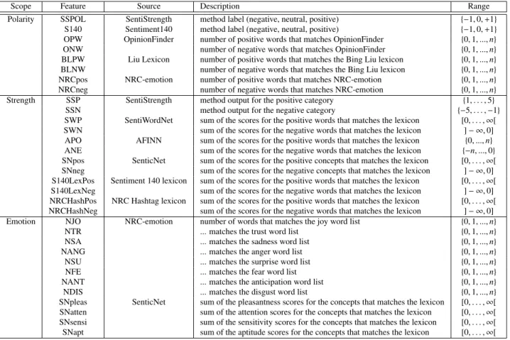
Scope Feature Source Description Range

Polarity SSPOL SentiStrength method label (negative, neutral, positive) {−1,0,+1}

S140 Sentiment140 method label (negative, neutral, positive) {−1,0,+1}

OPW OpinionFinder number of positive words that matches OpinionFinder {0,1, ...,n}

ONW number of negative words that matches OpinionFinder {0,1, ...,n}

BLPW Liu Lexicon number of positive words that matches the Bing Liu lexicon {0,1, ...,n}

BLNW number of negative words that matches the Bing Liu lexicon {0,1, ...,n}

NRCpos NRC-emotion number of positive words that matches NRC-emotion {0,1, ...,n}

NRCneg number of negative words that matches NRC-emotion {0,1, ...,n}

Strength SSP SentiStrength method output for the positive category {1, . . . ,5}

SSN method output for the negative category {−5, . . . ,−1}

SWP SentiWordNet sum of the scores for the positive words that matches the lexicon [0, . . . ,∞[

SWN sum of the scores for the negative words that matches the lexicon ]− ∞,0]

APO AFINN sum of the scores for the positive words that matches the lexicon {0, ...,n}

ANE sum of the scores for the negative words that matches the lexicon {−n, ...,0}

SNpos SenticNet sum of the scores for the positive concepts that matches the lexicon [0, . . . ,∞[

SNneg sum of the scores for the negative concepts that matches the lexicon ]− ∞,0]

S140LexPos Sentiment 140 lexicon sum of the scores for the positive words that matches the lexicon [0, . . . ,∞[

S140LexNeg sum of the scores for the negative words that matches the lexicon ]− ∞,0]

NRCHashPos NRC Hashtag lexicon sum of the scores for the positive words that matches the lexicon [0, . . . ,∞[

NRCHashNeg sum of the scores for the negative words that matches the lexicon ]− ∞,0]

Emotion NJO NRC-emotion number of words that matches the joy word list {0,1, ...,n}

NTR ... matches the trust word list {0,1, ...,n}

NSA ... matches the sadness word list {0,1, ...,n}

NANG ... matches the anger word list {0,1, ...,n}

NSU ... matches the surprise word list {0,1, ...,n}

NFE ... matches the fear word list {0,1, ...,n}

NANT ... matches the anticipation word list {0,1, ...,n}

NDIS ... matches the disgust word list {0,1, ...,n}

SNpleas SenticNet sum of the pleasantness scores for the concepts that matches the lexicon [0, . . . ,∞[

SNatten sum of the attention scores for the concepts that matches the lexicon [0, . . . ,∞[

SNsensi sum of the sensitivity scores for the concepts that matches the lexicon [0, . . . ,∞[

SNapt sum of the aptitude scores for the concepts that matches the lexicon [0, . . . ,∞[

Table 1: Sentiment-based features can be grouped into three classes of scope: Polarity, Strength, and Emotion.

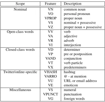
We also calculated part-of-speech (POS) features based on the frequency of each POS tag found in the message. The tagging task was done through the Carnegie Mellon University (CMU) Twitter NLP tool4_{which is focused on} informal, online conversational messages such as tweets. These features are summarized in Table 2 and can be grouped into the following categories: nominal words, open and closed class words, Twitter specific and miscellaneous.

(6)

Scope Feature Description

Nominal VN common noun

VO personal pronoun

VPROP proper noun

VS nominal + possessive

VZ proper noun + possessive

Open-class words VV verb

VA adjective

VR adverb

VI interjection

Closed-class words VD determiner

VP pre or postposition

VAND conjunction

VT verb particle

VX predeterminers

Twitter/online-specific VHASH hashtag

VARRO @ - at mention

VU URL or email address

VE emoticon

Miscellaneous V$ numeral

VPUNCT punctuation

VG foreign words

Table 2: Part-of-speech-based features.

3.1. Meta-level Features

OpinionFinder Lexicon. TheOpinionFinder Lexicon is a polarity oriented lexical resource created by Wilson et al. [33]. It is an extension of the Multi-Perspective Question-Answering dataset (MPQA), that includes phrases and subjective sentences. A group of human annotators tagged each sentence according to the polarity classes: positive, negative, neutral. The lexicon also includes 17 words with mixed positive and negative polarities tagged as “both”, which were omitted in this work. A pruning phase was conducted over the dataset to eliminate tags with low agree-ment. Thus, a list of sentences and single words was consolidated with their polarity tags. In this study we consider single words (unigrams) tagged as positive or negative, that correspond to a list of 6,884 English words. We extract from each tweet two features related to the OpinionFinder lexicon,OpinionFinder Positive Words(OPW) and Opin-ionFinder Negative Words(ONW), these are the numbers of positive and negative words of the tweet that matche the OpinionFinder lexicon, respectively.

Bing Liu’s Opinion Lexicon. This Lexicon is maintained and distributed by Bing Liu5and was used in several papers authored or co-authored by him [18]. The lexicon is polarity oriented and is formed by 2,006 positive words and 4,683 negative words. It includes misspelled words, slang words as well as some morphological variants. As is done in OpinionFinder, we extract the featuresBing Liu Positive Words(BLPW) andBing Liu Negative Words(BLNW). AFINN Lexicon. This lexicon is based on the Affective Norms for English Wordslexicon (ANEW) proposed by Bradley and Lang [3]. ANEW provides emotional ratings for a large number of English words. These ratings are calculated according to the psychological reaction of a person to a specific word, being “valence” the most useful value for sentiment analysis. “Valence” ranges in the scale from pleasant to unpleasant. ANEW was released before the rise of microblogging and hence, many slang words commonly used in social media were not included. Considering that there is empirical evidence about significant differences between microblogging words and the language used in other domains [2] a new version of ANEW was required. Inspired by ANEW, Nielsen [23] created theAFINNlexicon, which is more focused on the language used in microblogging platforms. The word list includes slang and obscene words and also acronyms and Web jargon. Positive words are scored from 1 to 5 and negative words from -1 to -5.

(7)

Thus, this lexicon is useful for strength estimation. The lexicon includes 2,477 English words. We extract from each tweet two features related to the AFINN lexicon:AFINN Positivity(APO) andAFINN Negativity(ANE), that are the sum of the ratings of positive and negative words of the tweet that matches the AFINN lexicon, respectively. SentiWordNet Lexicon. SentiWordNet 3.0 (SWN3) is a lexical resource for sentiment classification introduced by Baccianella et al. [1], that is an improvement over the original SentiWordNet proposed by Esuli and Sebastiani [12]. SentiWordNet is an extension ofWordNet, the well-known English lexical database where words are clustered into groups of synonyms known assynsets[19]. In SentiWordNet each synset is automatically annotated in the range [0,1] according to positivity, negativity and neutrality. These scores are calculated using semi-supervised algorithms. The resource is available for download6_{. In order to extract strength scores from SentiWordNet, we use word scores to} compute a real value from -1 (extremely negative) to 1 (extremely positive), where neutral words receive a zero score. We extract from each tweet two features related to the SentiWordnet lexicon,SentiWordnet Positiveness(SWP) and SentiWordnet Negativeness(SWN), that are the sum of the scores of positive and negative words of the tweet that matches the SentiWordnet lexicon, respectively.

NRC-emotion. NRC word-emotion association Lexicon includes a large set of human-provided words with their emo-tional tags. By conducting a tagging process in the crowdsourcing Amazon Mechanical Turk platform, Mohammad and Turney [20] created a word lexicon that contains more than 14,000 distinct English words annotated according to the Plutchik wheel of emotions. These words can be tagged to multiple categories. Eight emotions were considered during the creation of the lexicon, joy-trust, sadness-anger, surprise-fear, and anticipation-disgust, which compounds four opposing pairs. Additionally, NRC words are tagged according to polarity classes positive and negative, which are also considered in this work. The word list is available on request7. We extract from each tweet eight emotion features:NRC Joy(NJO),NRC Trust(NTR),NRC Sadness(NSA),NRC Anger(NANG),NRC Surprise(NSU), NRC Fear(NFE),NRC Anticipation(NANT), andNRC Disgust(NDIS), and two polarity features:NRC positive (NRCpos) andNRC negative(NRCneg), that are the number of words of the tweet that matches each category. NRC-Hashtag. The NRC Hashtag Sentiment Lexicon is an automatically created sentiment lexicon which was built from a collection of 775,310 tweets that contain positive or negative hashtags such as #good, #excellent, #bad, and #terrible. The tweets are labeled as positive or negative according to the hashtag’s polarities. A sentiment score is calculated for all the words and bigrams found in the collection using the point wise mutual information (PMI) measure between each word and the corresponding polarity label of the tweet. This score is a strength oriented sentiment dimension that ranges from -5 to 5. A positive value indicates a positive sentiment and a negative value indicates the opposite. The resource was created by the NRC-Canada team that won the SemEval task [21] and is available for download8_{. From each tweet we extract the features}_{NRC-Hashtag Positivity}_{(NRCHashPos) and} NRC-Hashtag Negativity(NRCHashNeg) that are the sum of scores of positive and negative words of the tweet that match the unigram list of the lexicon, respectively.

Sentiment140 Lexicon. This lexicon was also provided by theNRC-Canada team and was created following the same approach used for creating theNRC-Hashtag lexicon. Instead of using hashtags as tweet labels, a corpus of 1.6 million tweets with positive and negative emoticons was used to calculate the sentiment words. The tweet collection is the same one as the one used to train theSentiment140method in [13]. The lexicon is used to extract the strength oriented featuresS140Lex Positivity(S140LexPos) andS140Lex Negativity(S140Lex Positivity) which are calculated in the same manner as the features from theNRC-Hashtag.

Sentiment140 Method. Sentiment1409_{is a Web application that classifies tweets according to their polarity. The} eval-uation is performed using the distant supervision approach proposed by Go et al. [13] that was previously discussed in the related work section. The approach relies on supervised learning algorithms. Due to the difficulty of obtaining

6_{http://sentiwordnet.isti.cnr.it/}

7_{mailto: [email protected]}

8

http://www.umiacs.umd.edu/˜saif/WebDocs/NRC-Hashtag-Sentiment-Lexicon-v0.1.zip

(8)

a large-scale training dataset for this purpose, the problem is tackled using positive and negative emoticons and noisy labels. The method provides an API10_{that allows the classification of tweets to positive, negative and neutral polarity} classes. We extract from each tweet one feature related to the Sentiment140 output,Sentiment140class (S140), that corresponds to the output returned by the method.

SentiStrength Method. SentiStrength is a lexicon-based sentiment evaluator that is especially focused on short social Web texts written in English [30]. SentiStrength considers linguistic aspects of the passage such as a negating word list and an emoticon list with polarities. The implementation of the method can be freely used for academic purposes and is available for download11_{. For each passage to be evaluated, the method returns a positive score, from 1 (not} positive) to 5 (extremely positive), a negative score, from -1 (not negative) to -5 (extremely negative), and a neutral label taking the values: -1 (negative), 0 (neutral), and 1 (positive). We extract from each tweet three features related to the SentiStrength method:SentiStrength Negativity(SSN) andSentiStrength Positivity(SSP), that correspond to the strength scores for the negative and positive classes, respectively, andSentiStrength Polarity (SSPOL), a polarity-oriented feature corresponding to the neutral label.

SenticNet Method. SenticNet 2 [5] is a concept-based sentiment analysis method that follows thesentic computing paradigm. In contrast to traditional sentiment analysis approaches that perform a syntactic-level analysis of natural language texts, sentic computing techniques exploit AI and Semantic Web techniques to conduct a semantic-level analysis. SenticNet extracts both sentiment and semantic information from over 14,000 common sense knowledge concepts found in the message. The concepts are extracted using a graph-based technique. The method returns sentiment variables associated with each of the concepts found in the message: the polarity score, and the sentic vector. The polarity score is a real value similar to strength polarity values provided by other methods. The sentic vector is composed of emotion-oriented scores regarding the following emotions: pleasantness, attention, sensitivity and aptitude. These dimensions are based on the Hourglass model of emotions [7], which in turn, is inspired by Plutchik’s studies on human emotions. SenticNet concepts as well as the sentic parser are, available to download12_.

The features extracted from SenticNet areSenticNet Positivity(SNpos) andSenticNet Negativity(SNneg) that are the sum of the polarity of positive and negative concepts found on the message respectively. Additionally, we extract the following emotion-oriented features:SenticNet Pleasantness(SNpleas),SenticNet Attention(SNatten), SenticNet Sensitivity(SNsensi), and SenticNet Aptitude (SNapt) that are the sum of the scores of each sentic dimension for all the concepts found in the message.

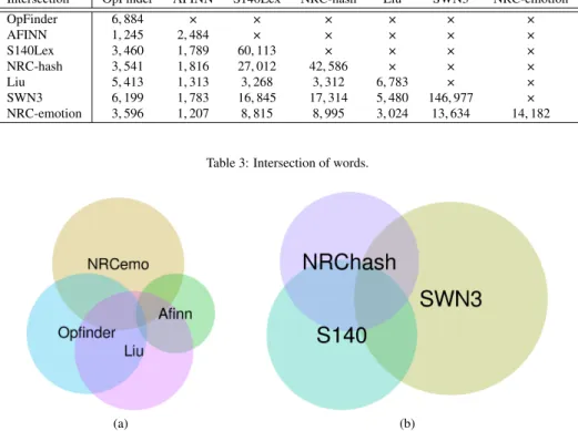
4. Experiments 4.1. Lexicon Analysis

In this section we study the interaction between the different lexical resources considered in this work: SWN3, NRC-emotion, OpinionFinder, AFINN, Liu Lexicon, NRC-Hashtag, and S140Lex. The aim of this study is to under-stand which type of information is provided by these resources and how they are related to each other. The lexicons may be compared according to different criteria: their sentiment scope, the approach used to build them, and the words that they contain. Regarding the sentiment scope we have two polarity-oriented resources: OpinionFinder and Liu, four strength-oriented resources: AFINN, SWN3, NRC-hash, and S140Lex, and one emotion-oriented lexicon: NRC-emotion, which also provides polarity values.

Regarding the mechanisms used to build the lexicons, we have three categories: resources created manually, re-sources created semi-automatically, and rere-sources created completely automatically. The lexicons Liu, AFINN, Opin-ionFinder, and NRC-emotion were manually created resources. They were created by taking words from different sources, and their sentiment values were mostly determined by human judgments using tools such as crowdsourc-ing. SWN3 is a resource created semi-automatically, because its words were taken from a fixed resource (WordNet synsets), but its sentiment values were computed using a semi-supervised approach. Finally, the lexicons NRC-hash and S140Lex are resources created completely automatically, because its words and their sentiment values were jointly extracted from large collections of tweets in an automatic way.

10_{http://help.sentiment140.com/api}

11_{http://sentistrength.wlv.ac.uk/}

(9)

Intersection OpFinder AFINN S140Lex NRC-hash Liu SWN3 NRC-emotion OpFinder 6,884 × × × × × × AFINN 1,245 2,484 × × × × × S140Lex 3,460 1,789 60,113 × × × × NRC-hash 3,541 1,816 27,012 42,586 × × × Liu 5,413 1,313 3,268 3,312 6,783 × × SWN3 6,199 1,783 16,845 17,314 5,480 146,977 × NRC-emotion 3,596 1,207 8,815 8,995 3,024 13,634 14,182

Table 3: Intersection of words.

(a) (b)

Figure 1: Venn diagrams for the lexicons used in our experiments. a) lexicons created manually, and b) lexicons created semi-automatically and completely automatically.

The number of words that overlap between each pair of resources are shown in Table 3. From the table we can see that resources created semi-automatically and completely automatically, SWN3, NRC-hash, and S140Lex are much larger than resources created manually. This is intuitive, because while SWN3 was created from WordNet, which is a large lexical database, NRC-hash and S140Lex are both formed by all the different words found in their respective large collections of tweets. The word interaction of the lexicons created manually is better represented in the Venn diagram shown in Figure 1a. We observe that both polarity-oriented lexicons Liu and OpinionFinder present an important overlap between each other. Figure 1b shows the interaction of lexicons created semi-automatically and completely automatically. We can see that the overlap between both lexicons built from Twitter data is greater than the overlap they have with SWN3. This suggests that Twitter-made lexicons contain several expressions that are specific to Twitter.

The level ofuniquenessof each resource is shown in Table 4. This value corresponds to the fraction of words of the lexicon that are not included in any of the remaining resources. We can see that as lexicons created manually tend to have a low uniqueness, resources created semi-automatically and completely automatically tend to have an important level of uniqueness. Nevertheless, regarding the AFINN lexicon, despite being the smallest lexicon created manually, it contains several words that are not included in other lexicons. This is because AFINN contains several Internet acronyms and slang words.

We also studied the level ofneutralityof each resource, as is shown in the second column of Table 4. This value corresponds to the fraction of words of the lexicon marked as neutral, and hence, doess not provide relevant sentiment information. The criteria for determining if a word is neutral varies from one lexicon to another. In OpinionFinder neutral words are marked explicitly. Conversely, AFINN and Liu do not have neutral words. For the case of S140Lex and NRC-hash we consider as neutral, all the words in which the absolute value of its score was less than one. In a similar manner, we consider as neutral, all the words of SWN3 with a zero sentiment score. Finally, for NRC-emotion we consider as neutral, all words that are part of the lexicon and are not associated with any emotion or polarity class. Regarding the lexicons created manually we see that only NRC-emotion has a significant level of neutrality.

(10)

Lexicon Uniqueness Neutrality OpFinder 0.01 0.06 AFINN 0.19 0.00 S140Lex 0.51 0.62 NRC-hash 0.29 0.72 Liu 0.05 0.00 SWN3 0.82 0.74 NRC-emotion 0.01 0.54

Table 4: Neutrality and uniqueness of each Lexicon.

Resources created semi-automatically and completely automatically present the highest levels of neutrality. This is because they include all the words from the sources used to create them (WordNet and Twitter). Then, as WordNet and Twitter contain a great diversity of words or expressions, it is expected for their derived lexicons to contain many words with no sentiment orientation.

In addition to comparing the words contained in the lexicons, we also compared the level of agreement between them. We extracted the 609 words that intersect all the different lexicons. Afterwards, all the sentiment values assigned by each lexicon were converted to polarity categories: positive and negative. For strength-oriented lexicons we converted positive and negative scores to positive and negative labels respectively. Then, for NRC-emotion we used the polarity dimensions provided by the lexicon. The agreement between two lexicons is calculated as the fraction of words from the global intersection where both lexicons assigned the same polarity label to the word. The levels of agreement between all lexicons are shown in Table 5. From the Table we see that the agreement between lexicons created manually is very high, indicating that different human judgements tend to agree with each other. On the other hand, large lexicons created semi-automatically and completely automatically shows a high level of disagreement with the human-made lexicons and even greater levels of disagreement between each other. That means, that these resources, despite being larger, tend to provide noisy information, which is far from being consolidated.

Agreement OpFinder AFINN S140Lex NRC-hash Liu SWN3 NRC-emotion

OpFinder 1 × × × × × × AFINN 0.99 1 × × × × × S140Lex 0.82 0.82 1 × × × × NRC-hash 0.79 0.79 0.72 1 × × × Liu 0.99 0.99 0.82 0.79 1 × × SWN3 0.85 0.76 0.66 0.64 0.84 1 × NRC-emotion 0.99 0.99 0.84 0.82 0.99 0.86 1

Table 5: Agreement of lexicons.

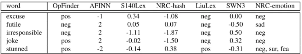
From the 609 words that are contained in all the lexicons, 292 of them present at least one disagreement between two different lexicons. A group of words presenting disagreements along the different types of lexicons is presented in Table 6. We can see that words such as “excuse”, “joke”, and “stunned” may be used to express either positive and negative opinions, depending on the context. Considering that it is very hard to associate all the words with a single polarity class, we think that emotion tags explain in a better manner the diversity of sentiment states triggered by these kinds of words. For instance, the word “stunned” which is associated with both positive and negative polarities, is also associated with surprise and fear emotions. As this word would more likely be negative in a context of “fear”, it would also be more likely to be “positive” in a context of “surprise”.

All the insights revealed from this analysis indicate that the resources considered in this work complement each other, providing different sentiment information and also present different levels of noise. A previous study on the relationship between different opinion lexicons was presented as a tutorial by Christopher Potts at the Sentiment Analysis Symposium13_.

(11)

word OpFinder AFINN S140Lex NRC-hash LiuLex SWN3 NRC-emotion

excuse pos -1 0.34 -1.08 neg 0.00 neg

futile neg 2 0.05 0.07 neg -0.50 sad

irresponsible neg 2 -1.11 -1.87 neg 0.50 neg

joke pos 2 -0.02 -1.50 neg 0.32 neg

stunned pos -2 -0.14 0.38 pos -0.31 neg, sur, fea

Table 6: Sentiment values for different words.

4.2. Sentiment Classification

We follow a supervised learning approach for which we model each tweet as a vector of sentiment features. A dataset of manually annotated tweets is required for training and evaluation purposes. Two classification tasks are considered: subjectivity and polarity classification. In the former, tweets are classified as subjective (non-neutral) or objective (neutral), and in the latter as positive or negative. Moreover, positive and negative tweets are considered as subjective.

Once the feature vectors of all the tweets from the dataset have been extracted, they are used together with the annotated sentiment labels as input for supervised learning algorithms. Several learning algorithms can be used to fulfill this task, e.g., naive Bayes, SVM, decision trees. Finally, the resulting learned function can be used to automatically infer the sentiment label regarding an unseen tweet.

4.2.1. Training and Testing Datasets

We consider three collections of labeled tweets for our experiments: Stanford Twitter Sentiment(STS)14_{, which} was used by Go et al. [13] in their experiments,Sanders15_{, and SemEval}16_{, which provide training and testing datasets} for a range of interesting and challenging semantic analysis problems, among them, tweets with human annotations for subjectivity and polarity prediction. Each tweet includes apositive,negativeorneutraltag. Table 7 summarizes the three datasets.

STS Sanders SemEval

#negative 177 636 3,639

#neutral 139 2,429 4,585

#positive 182 560 1,458

#total 498 3,625 9,682

Table 7: Datasets statistics.

STS and Sanders exhibit unbalance between the number of subjective/neutral instances. Something similar occurs in SemEval between the number of positive/negative instances. We balance these training instances by conducting resampling with replacement, avoiding the creation of models biased toward a specific class. The balanced datasets are available upon request.

Negative and positive tweets were considered as subjective. Neutral tweets were considered as objective. Sub-jective/objective tags favor the evaluation of subjectivity detection. For polarity detection tasks, positive and negative tweets were considered, discarding neutral tweets.

4.2.2. Feature Analysis

For each tweet of the three datasets we compute the features summarized in Table 1 and Table 2.

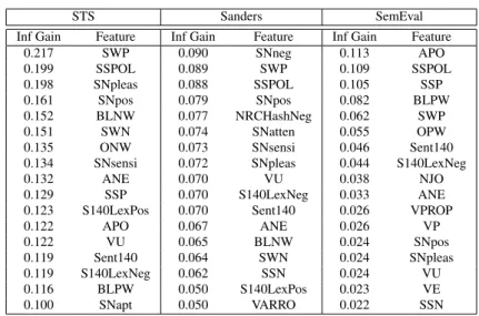
As a first analysis we explore how well each feature splits each dataset regarding polarity and subjectivity detection tasks. We do this by calculating the information gain criterion of each feature in each category. The information gain criterion measures the reduction of the entropy within each class after performing the best split induced by the feature. Table 8 shows the information gain values obtained for the subjectivity detection task and Table 9 for polarity.

14_{http://cs.stanford.edu/people/alecmgo/trainingandtestdata.zip}

15_{http://www.sananalytics.com/lab/twitter-sentiment/}

(12)

STS Sanders SemEval

Inf Gain Feature Inf Gain Feature Inf Gain Feature

0.217 SWP 0.090 SNneg 0.113 APO 0.199 SSPOL 0.089 SWP 0.109 SSPOL 0.198 SNpleas 0.088 SSPOL 0.105 SSP 0.161 SNpos 0.079 SNpos 0.082 BLPW 0.152 BLNW 0.077 NRCHashNeg 0.062 SWP 0.151 SWN 0.074 SNatten 0.055 OPW

0.135 ONW 0.073 SNsensi 0.046 Sent140

0.134 SNsensi 0.072 SNpleas 0.044 S140LexNeg

0.132 ANE 0.070 VU 0.038 NJO

0.129 SSP 0.070 S140LexNeg 0.033 ANE

0.123 S140LexPos 0.070 Sent140 0.026 VPROP

0.122 APO 0.067 ANE 0.026 VP 0.122 VU 0.065 BLNW 0.024 SNpos 0.119 Sent140 0.064 SWN 0.024 SNpleas 0.119 S140LexNeg 0.062 SSN 0.024 VU 0.116 BLPW 0.050 S140LexPos 0.023 VE 0.100 SNapt 0.050 VARRO 0.022 SSN

Table 8: Ranked features for subjectivity classification.

STS Sanders SemEval

Inf Gain Feature Inf Gain Feature Inf Gain Feature

0.318 S140LexNeg 0.323 SWN 0.261 S140LexNeg

0.318 Sent140 0.260 NRCHashNeg 0.261 Sent140

0.283 SSPOL 0.220 Sent140 0.190 SSPOL

0.260 BLNW 0.220 S140LexNeg 0.178 ANE

0.219 SSP 0.199 S140LexPos 0.151 NRCHashNeg

0.207 SSN 0.179 SNsensi 0.148 BLNW

0.204 ANE 0.172 SSPOL 0.142 S140LexPos

0.193 S140LexPos 0.162 NRCHashPos 0.137 SSP

0.172 APO 0.141 SNapt 0.131 SWN

0.152 BLPW 0.135 SNneg 0.131 APO

0.141 SWN 0.134 SSP 0.119 SSN

0.139 ONW 0.128 SNpleas 0.108 NRCHashPos

0.129 SNneg 0.126 ANE 0.107 BLPW

0.106 NRCHashPos 0.124 APO 0.098 SNpleas

0.099 NRCHashNeg 0.119 BLNW 0.095 SNneg

0.090 SNpleas 0.108 SSN 0.082 ONW

0.082 OPW 0.104 BLPW 0.070 NJO

Table 9: Ranked features for polarity classification.

As shown in Table 8 and Table 9, good subjectivity and polarity splits are achieved by using the outcomes of SSPOL and Sent140. Lexical-based features retrieved from SentiWordNet, OpinionFinder and AFINN are very useful for polarity and subjectivity detection. We observe also that features retrieved from SenticNet are useful for both tasks. In the case of subjectivity detection, the use of POS-based features is also useful, but is useless for polarity detection. Regarding information gain values for subjectivity, we observe that the best splits are achieved in STS. On the other hand, Sanders is very hard to split. Regarding polarity, we observe that the best splits are achieved in STS and Sanders, though SemEval is hard to split.

By analyzing the scope, we observe that polarity and strength-based features are the most informative for both tasks. This fact is intuitive because the target variables belong to the same scope. In addition, POS-based features are useful for subjectivity. Finally, although emotion features from NRC-emotion lexicon provide almost no information for subjectivity, the emotionjoyis able to provide some information for the polarity classification task.

We use information gain as a criterion for feature selection. Information gain allows us to use proper features for label separation. As this set of features comes from different lexical resources, this approach can be viewed as a

(13)

feature fusion approach. To explore the combination at the level of features, we discard the use of SSPOL and Sent140 in our classifiers, avoiding the combination of labels. In the next section we illustrate that this design decision allows us to elude the effect of label clashes, which is very significant in our evaluation datasets. Accordingly, SSPOL and Sent140 are only considered as baselines in our experiments.

4.2.3. Clash analysis

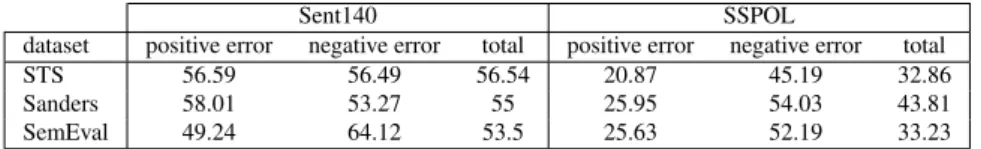
We conduct a label comparison between baselines and each evaluation dataset used in our experiments. We compare the nominal labels provided by the datasets, and the labels of Sent140 and SSPOL. The comparison was performed by splitting each dataset into two subsets for each task: 1) Neutral and subjective labeled instances, and 2) Positive and negative labeled instances. For each split, we count the number of label clashes. Then, an error rate (number of mismatches over total number of labeled instances) considered over the total amount of instances per label was calculated. Tables 10 and 11 show error rates for subjectivity and polarity tasks, respectively.

Sent140 SSPOL

dataset neutral error subj error total neutral error subj error total

STS 9.35 53.76 41.36 31.65 18.11 21.88

Sanders 26.53 48.95 35.2 50.65 22.01 39.58

SemEval 26.91 48.96 38.52 44.31 18.83 30.9

Table 10: Number of clashes (percentage over number of labeled instances) per dataset for neutral and subjectivity errors for the baseline methods used in our evaluation.

Sent140 SSPOL

dataset positive error negative error total positive error negative error total

STS 56.59 56.49 56.54 20.87 45.19 32.86

Sanders 58.01 53.27 55 25.95 54.03 43.81

SemEval 49.24 64.12 53.5 25.63 52.19 33.23

Table 11: Number of clashes (percentage over number of labeled instances) per dataset for positive and negative errors for the baseline methods used in our evaluation.

Tables 10 and 11 show that error rates are very significant. In particular, Sent140 consistently exhibits very high errors for the polarity task, with rates over the 50%, illustrating its incapacity to generalize to these datasets. On the other hand, SSPOL shows better properties for the detection of positive tweets, but poor abilities for negativity detection. These high error rates explain why these methods are not suitable for subjectivity detection, indicating that the combination of output labels introduces label inconsistency, discouraging the use of label ensemble methods. 4.2.4. Lexical Diversity

In this section we argue that the use of multiple lexical resources offers benefits for sentiment analysis tasks. The rationale behind our approach is based on diversity. Multiple lexical resources can be used to describe an object (e.g., a tweet) in the hope that if one or more fail, the others will compensate for it by producing correct features. This principle had sustained it over the independence assumption. As lexical resources were independently created, errors are also independent.

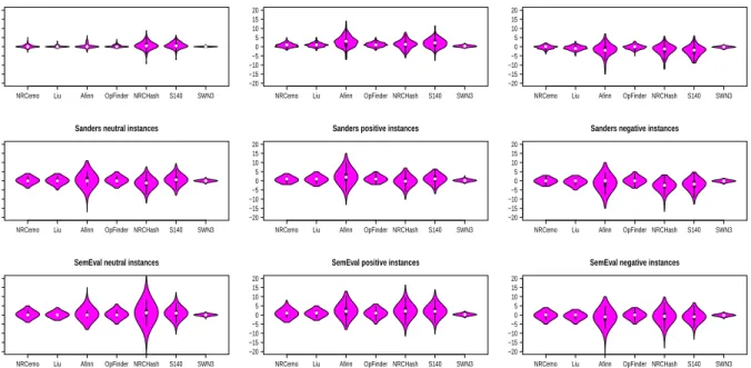
We explore diversity by showing the output scores of lexical resources in each dataset split (neutral, positive, and negative instances). Polarity or strength scores of each instance were calculated by adding positive and negative scores. Figure 2 shows these score distributions, using boxplots with density (a.k.a. vioplots).

Figure 2 allows us a side-by-side comparison between score distributions. We observe that in general, the median is located around zero for neutral instances, above zero for positive instances and below zero for negative instances, ratifying the correctness of several of the word hits. Regarding score variance, these plots show that the spread of AFINN, NRC-hash and S140Lex is bigger than the spread of NRC-emotion, Liu and OpFinder. Intuitively, this fact can be explained by the size of the lexicons. AFINN spreads more than NRC-hash and S140Lex in Sanders, but NRC-hash spreads more than AFINN and S140Lex in SemEval on neutral instances. The spread among these three

(14)

NRCemo Liu Afinn OpFinder NRCHash S140 SWN3 −20 −15 −10 −5 0 5 10 15 20 STS neutral instances

NRCemo Liu Afinn OpFinder NRCHash S140 SWN3 −20 −15 −10 −5 0 5 10 15 20 STS positive instances

NRCemo Liu Afinn OpFinder NRCHash S140 SWN3 −20 −15 −10 −5 0 5 10 15 20 STS negative instances

NRCemo Liu Afinn OpFinder NRCHash S140 SWN3 −20 −15 −10 −5 0 5 10 15 20

Sanders neutral instances

Sanders positive instances

Sanders negative instances

SemEval neutral instances

SemEval positive instances

SemEval negative instances

Figure 2: Neutral, positive and negative instances of each dataset used in our experiments and their polarity or strength score distributions (boxplots with densities, a.k.a. vioplots) in each lexical resource.

lexicons is very similar in positive and negative Sanders instances. We can conclude that polarity and strength scores vary in median and spread across the different datasets and lexical resources, offering multiple views of the same objects that can be combined using a feature-based fusion strategy.

4.2.5. Fusion of features for sentiment analysis

In this section we present the methodology we use to create our models for automatic subjectivity and polarity prediction for tweets. We do this by using labels and instances from STS, Sanders and SemEval. We train supervised classifiers to determine subjectivity at tweet level. For this supervised training task we use the labeled tweets obtained from each of the datasets. These labels consider two classes (SUBJECTIVE/NEUTRAL), discussed in Section 4.2.

We compare our classifiers against a number of strategies: Sent140 and SentiStrength Polarity (SSPOL), as base-line methods. We conduct a comparison with NRC-emotion, SenticNet, Liu lexicon, NRC-hash, S140Lex, AFINN, SWN3, and OpinionFinder.

We experimentally compare the performance of a number of learning algorithms: Naive Bayes, Logistic Regres-sion, Multilayer Perceptron, and Radial Basis Function SVM. All of the experiments are conducted using 10-fold cross-validation for evaluation.

The use of these learning algorithms allows for the exploration of different aspects of the datasets, such as their suitability for generalization or the presence/absence of non-linearities in the data.

We study how features contribute in the prediction of subjectivity and evaluate features by dividing them into the following subsets:

Polarity. Considers all of the features that are based on polarity estimates at tweet-level. This includes the features based on OpinionFinder, Bing Liu and NRC lexicons. For each of these lexicons we consider two features: number of positive and negative words. Table 1 shows a detailed description of these eight features.

Strength. Considers all the features that are based on strength estimates at tweet level. Table 1 shows a detailed description of these twelve features.

Emotion. Considers all the features that are based on emotion estimates at tweet level. This includes the features based on NRC-emotion, that is to say, the number of words that match each emotion list, which give us 8 features.

(15)

Also, those related to SenticNet, that consider the sum of the scores for each of the opinion aspects modeled by this method (pleasantness, attention, sensitivity and aptitude). These twelve features are described in Table 1.

POS. Considers all the features that are based on Part-Of-Speech estimates at tweet level. This includes the features based on TweetNLP, which give us the number of words in each tweet that match a given POS label. Tweet NLP considers five scopes, Three of them are related to conventional POS tags (Nominal, Open-class words, and closed-class words), another related to Twitter specific tags, and a last one related to punctuation. These five scopes contain twenty-one features described in Table 2.

We test combinations of feature subsets, selecting arbitrary sets of features with a best-first strategy based on information gain criteria. The best features and their information gain values are shown in Table 8. We observe that in each subset, SSPOL and S140 were selected as features. We exclude them from this subset because they are considered as methods, and their output ranges in the same label space as our learning task. Accordingly, each subset contains 15 features. In addition, we also test the use of all the features.

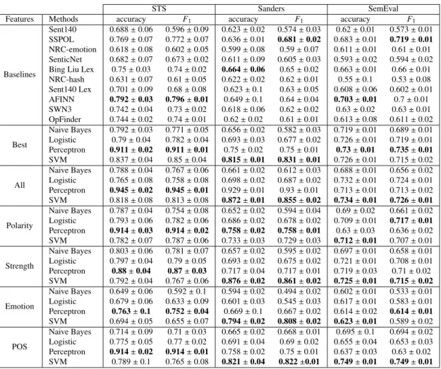
STS Sanders SemEval

Features Methods accuracy F1 accuracy F1 accuracy F1

Baselines

Sent140 0.688±0.06 0.596±0.09 0.623±0.02 0.574±0.03 0.62±0.01 0.573±0.01

SSPOL 0.769±0.07 0.772±0.07 0.636±0.01 0.681±0.02 0.683±0.01 0.719±0.01

NRC-emotion 0.618±0.08 0.602±0.05 0.599±0.08 0.59±0.07 0.611±0.01 0.61±0.01

SenticNet 0.682±0.07 0.673±0.02 0.611±0.09 0.605±0.03 0.593±0.02 0.594±0.02

Bing Liu Lex 0.75±0.03 0.74±0.02 0.664±0.06 0.65±0.02 0.663±0.01 0.66±0.01

NRC-hash 0.631±0.07 0.61±0.05 0.622±0.02 0.62±0.01 0.55±0.1 0.53±0.08 Sent140 Lex 0.701±0.09 0.68±0.08 0.623±0.1 0.63±0.05 0.608±0.06 0.602±0.01 AFINN 0.792±0.03 0.796±0.01 0.649±0.1 0.64±0.04 0.703±0.01 0.7±0.01 SWN3 0.742±0.04 0.73±0.02 0.618±0.06 0.62±0.02 0.63±0.02 0.63±0.01 OpFinder 0.744±0.02 0.74±0.01 0.62±0.02 0.61±0.01 0.613±0.08 0.611±0.02 Best Naive Bayes 0.792±0.03 0.771±0.05 0.656±0.02 0.582±0.03 0.719±0.01 0.689±0.01 Logistic 0.79±0.04 0.782±0.04 0.693±0.03 0.677±0.02 0.726±0.01 0.719±0.01 Perceptron 0.911±0.02 0.911±0.01 0.75±0.02 0.75±0.01 0.73±0.01 0.735±0.01 SVM 0.837±0.04 0.85±0.04 0.815±0.01 0.831±0.01 0.726±0.01 0.715±0.02 All Naive Bayes 0.788±0.04 0.767±0.06 0.661±0.02 0.612±0.03 0.688±0.01 0.656±0.02 Logistic 0.765±0.08 0.758±0.08 0.698±0.02 0.687±0.02 0.732±0.01 0.724±0.01 Perceptron 0.945±0.02 0.945±0.01 0.929±0.01 0.93±0.01 0.713±0.01 0.713±0.02 SVM 0.818±0.08 0.813±0.08 0.872±0.01 0.855±0.02 0.734±0.01 0.726±0.01 Polarity Naive Bayes 0.787±0.04 0.754±0.08 0.652±0.02 0.594±0.04 0.69±0.02 0.661±0.02 Logistic 0.793±0.06 0.782±0.06 0.686±0.02 0.678±0.02 0.709±0.01 0.717±0.01 Perceptron 0.914±0.03 0.914±0.02 0.758±0.02 0.758±0.01 0.63±0.03 0.636±0.02 SVM 0.782±0.07 0.787±0.06 0.733±0.03 0.729±0.03 0.712±0.01 0.707±0.01 Strength Naive Bayes 0.803±0.06 0.781±0.07 0.657±0.02 0.595±0.02 0.697±0.01 0.658±0.01 Logistic 0.797±0.04 0.79±0.05 0.693±0.02 0.675±0.02 0.721±0.01 0.708±0.01 Perceptron 0.88±0.04 0.87±0.03 0.717±0.04 0.717±0.01 0.719±0.03 0.71±0.02 SVM 0.792±0.04 0.767±0.06 0.876±0.02 0.861±0.02 0.725±0.01 0.715±0.02 Emotion Naive Bayes 0.649±0.06 0.592±0.1 0.594±0.02 0.494±0.02 0.602±0.01 0.533±0.01 Logistic 0.679±0.06 0.633±0.09 0.601±0.03 0.545±0.03 0.617±0.01 0.583±0.01 Perceptron 0.763±0.1 0.752±0.04 0.669±0.1 0.667±0.02 0.614±0.02 0.614±0.01 SVM 0.694±0.05 0.655±0.07 0.794±0.02 0.808±0.02 0.623±0.01 0.589±0.02 POS Naive Bayes 0.714±0.09 0.71±0.03 0.665±0.02 0.668±0.01 0.695±0.1 0.694±0.02 Logistic 0.775±0.05 0.77±0.02 0.691±0.04 0.69±0.02 0.655±0.04 0.653±0.03 Perceptron 0.914±0.02 0.914±0.01 0.758±0.02 0.75±0.01 0.637±0.03 0.63±0.02 SVM 0.789±0.1 0.765±0.08 0.821±0.04 0.822±0.01 0.749±0.01 0.749±0.01

Table 12: 10-fold cross-validation subjectivity classification performances.

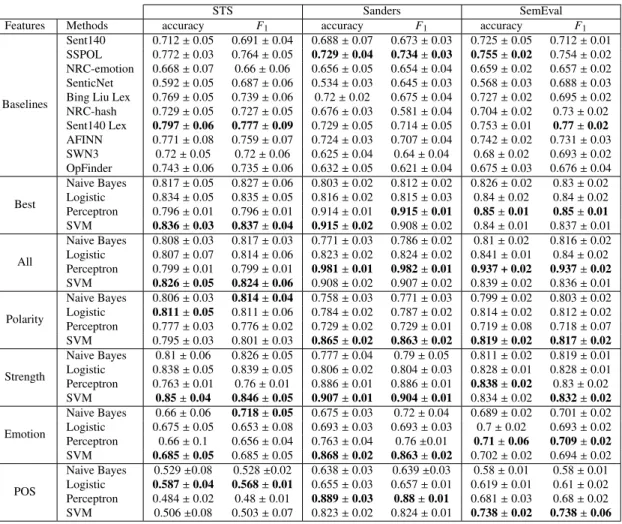
The results for the subjectivity classification task are shown in Table 12. The best baseline for STS and SemEval is AFINN. In the case of Sanders, the best baseline is Liu Lexicon. The combination of features outperforms the baselines by several accuracy and F-measure points. In particular, we observe that the use of the best features subset outperforms baselines and other feature subsets in STS and SemEval. In the case of Sanders, best results are achieved by using all the features, suggesting that this dataset is not well conditioned for generalization. We observe also that the best performance results are achieved by Perceptron and SVM learning algorithms, outperforming Logistic and Bayes learning methods by several accuracy points. This suggests the presence of non-linearities in the feature space.

(16)

For STS, best results are achieved by Perceptron using All and Best features. However, we observe that POS-based features are useful for this task, outperforming Best features performance. Something similar occurs in Sanders, where Best and All features outperform the other models by several points. In fact, we observe that the best result is achieved by Perceptron over the whole set of features. In this case we observe also that POS-based features are useful for this task, and that the use of Strength features in combination with SVMs offers good results. Regarding SemEval, the best results are achieved by combining Best features with Perceptron-based learning, without significant differences with an SVM model created over the whole feature set, suggesting that Best feature subset offers good generalization properties in this dataset. Once again, the use of POS features in combination with SVMs offers very good results.

We now study how features contribute to the prediction of polarity. We train supervised classifiers to determine polarity at tweet level. For this supervised training task we use the labeled tweets obtained from each of the datasets. These labels consider two classes (POSITIVE/NEGATIVE), discussed in Section 4.2. We evaluate features by divid-ing them into the same subsets considered in the former evaluation. In addition, we consider the same baselines.

We also test combinations of feature subsets, selecting arbitrary sets of features with a best-first strategy based on information gain criteria. The best features and their information gain values are shown in Table 9. As was done for subjectivity, we exclude SSPOL and S140 from this subset. In this way, each subset contains 15 features. We observe that for this task, POS-based features do not show good properties regarding information gain, being outperformed for feature selection by lexicon-based features. In addition, we test the use of all the features. Table 13 shows the results for the subjectivity classification task.

STS Sanders SemEval

Features Methods accuracy F1 accuracy F1 accuracy F1

Baselines

Sent140 0.712±0.05 0.691±0.04 0.688±0.07 0.673±0.03 0.725±0.05 0.712±0.01

SSPOL 0.772±0.03 0.764±0.05 0.729±0.04 0.734±0.03 0.755±0.02 0.754±0.02

NRC-emotion 0.668±0.07 0.66±0.06 0.656±0.05 0.654±0.04 0.659±0.02 0.657±0.02

SenticNet 0.592±0.05 0.687±0.06 0.534±0.03 0.645±0.03 0.568±0.03 0.688±0.03

Bing Liu Lex 0.769±0.05 0.739±0.06 0.72±0.02 0.675±0.04 0.727±0.02 0.695±0.02

NRC-hash 0.729±0.05 0.727±0.05 0.676±0.03 0.581±0.04 0.704±0.02 0.73±0.02 Sent140 Lex 0.797±0.06 0.777±0.09 0.729±0.05 0.714±0.05 0.753±0.01 0.77±0.02 AFINN 0.771±0.08 0.759±0.07 0.724±0.03 0.707±0.04 0.742±0.02 0.731±0.03 SWN3 0.72±0.05 0.72±0.06 0.625±0.04 0.64±0.04 0.68±0.02 0.693±0.02 OpFinder 0.743±0.06 0.735±0.06 0.632±0.05 0.621±0.04 0.675±0.03 0.676±0.04 Best Naive Bayes 0.817±0.05 0.827±0.06 0.803±0.02 0.812±0.02 0.826±0.02 0.83±0.02 Logistic 0.834±0.05 0.835±0.05 0.816±0.02 0.815±0.03 0.84±0.02 0.84±0.02 Perceptron 0.796±0.01 0.796±0.01 0.914±0.01 0.915±0.01 0.85±0.01 0.85±0.01 SVM 0.836±0.03 0.837±0.04 0.915±0.02 0.908±0.02 0.84±0.01 0.837±0.01 All Naive Bayes 0.808±0.03 0.817±0.03 0.771±0.03 0.786±0.02 0.81±0.02 0.816±0.02 Logistic 0.807±0.07 0.814±0.06 0.823±0.02 0.824±0.02 0.841±0.01 0.84±0.02 Perceptron 0.799±0.01 0.799±0.01 0.981±0.01 0.982±0.01 0.937 + 0.02 0.937±0.02 SVM 0.826±0.05 0.824±0.06 0.908±0.02 0.907±0.02 0.839±0.02 0.836±0.01 Polarity Naive Bayes 0.806±0.03 0.814±0.04 0.758±0.03 0.771±0.03 0.799±0.02 0.803±0.02 Logistic 0.811±0.05 0.811±0.06 0.784±0.02 0.787±0.02 0.814±0.02 0.812±0.02 Perceptron 0.777±0.03 0.776±0.02 0.729±0.02 0.729±0.01 0.719±0.08 0.718±0.07 SVM 0.795±0.03 0.801±0.03 0.865±0.02 0.863±0.02 0.819±0.02 0.817±0.02 Strength Naive Bayes 0.81±0.06 0.826±0.05 0.777±0.04 0.79±0.05 0.811±0.02 0.819±0.01 Logistic 0.838±0.05 0.839±0.05 0.806±0.02 0.804±0.03 0.828±0.01 0.828±0.01 Perceptron 0.763±0.01 0.76±0.01 0.886±0.01 0.886±0.01 0.838±0.02 0.83±0.02 SVM 0.85±0.04 0.846±0.05 0.907±0.01 0.904±0.01 0.834±0.02 0.832±0.02 Emotion Naive Bayes 0.66±0.06 0.718±0.05 0.675±0.03 0.72±0.04 0.689±0.02 0.701±0.02 Logistic 0.675±0.05 0.653±0.08 0.693±0.03 0.693±0.03 0.7±0.02 0.693±0.02 Perceptron 0.66±0.1 0.656±0.04 0.763±0.04 0.76±0.01 0.71±0.06 0.709±0.02 SVM 0.685±0.05 0.685±0.05 0.868±0.02 0.863±0.02 0.702±0.02 0.694±0.02 POS Naive Bayes 0.529±0.08 0.528±0.02 0.638±0.03 0.639±0.03 0.58±0.01 0.58±0.01 Logistic 0.587±0.04 0.568±0.01 0.655±0.03 0.657±0.01 0.619±0.01 0.61±0.02 Perceptron 0.484±0.02 0.48±0.01 0.889±0.03 0.88±0.01 0.681±0.03 0.68±0.02 SVM 0.506±0.08 0.503±0.07 0.823±0.02 0.824±0.01 0.738±0.02 0.738±0.06

Table 13: 10-fold cross-validation polarity classification performances.

(17)

combination of features exceeds the baselines performance by several accuracy and F-measure points. In particular, we observe that the use of the best features subset outperforms baselines and other feature subsets in STS and SemEval. We observe in this task that the use of the full feature space with a Perceptron-based learning strategy outperforms best feature-based models in Sanders and SemEval. This fact suggests that polarity prediction is a difficult to address problem and that the features explored in this evaluation cannot generalize to the whole dataset. We observe also that the performance gap between Bayes/Logistic and Perceptron/SVM is lower than the one observed for subjectivity, suggesting that the presence of non-linearities in the feature space for this task is insignificant. Regarding subset fea-tures, we observe that the use of strength-based features is useful for this task, outperforming polarity-based features in the three datasets. Emotion-based features are not helpful for this task, suggesting that polarity and emotion-based characterizations are different problems. Likewise, we observe that POS-based features are not useful for this task. 4.2.6. Error analysis

In this section we analyze error instances in each dataset used in our experiments. We conduct a comparison of the intra-variance of each feature vector between hits and error instances. The intra-variance of each feature vector is the variance calculated over the set of values that the feature vector registers for a specific data instance. Intuitively, the intra-variance decreases as lexical resources achieve more agreements. Thus, a high intra variance is a measure of disagreement. For each testing instance, we calculate the variance across the features used in the best features-based model. Figure 3 shows variance distributions for error and hits instances using boxplots with densities (a.k.a. violin plots). Errors Hits 0 5 10 15 20 25 30 35 40

STS subjectivity feature variance