Département des Sciences Économiques
de l'Université catholique de Louvain
Bayesian inference for the mixed
conditional heteroskedasticity model
L. Bauwens and J. V.K. Rombouts
CORE DISCUSSION PAPER 2005/85
BAYESIAN INFERENCE FOR THE MIXED CONDITIONAL HETEROSKEDASTICITY MODEL
L. Bauwens1 and J.V.K. Rombouts1 December 1, 2005
Abstract
We estimate by Bayesian inference the mixed conditional heteroskedasticity model of (Haas, Mittnik, and Paolella 2004a). We construct a Gibbs sampler algorithm to compute posterior and predictive densities. The number of mixture components is selected by the marginal likelihood criterion. We apply the model to the SP500 daily returns.
Keywords: Finite mixture, ML estimation, Bayesian inference, Value at Risk.
JEL Classification: C11, C15, C32
1CORE and Department of Economics, Universit´e Catholique de Louvain. 2HEC Montr´eal, CIRANO, CIRPEE and CREF.
We thank Viorel Maxim for excellent research assistance and Arie Preminger for his comments. Bauwens’s work was supported in part by the European Community’s Human Potential Programme under contract HPRN-CT-2002-00232, MICFINMA and by a FSR grant from UCL. Rombouts’s work was supported by a HEC Montr´eal Fonds de d´emarrage and by the Centre for Research on e-Finance.
This text presents research results of the Belgian Program on Interuniversity Poles of Attraction initiated by the Belgian State, Prime Minister’s Office, Science Policy Programming. The scientific responsibility is assumed by the authors.
1
Introduction
Finite mixture models, see e.g. (McLachlan and Peel 2000), are more and more used in statistics and econometrics. Their main advantage lies in the flexibility they provide in model specification, compared to the use of a more simple distribution. On the other hand, these models are more difficult to estimate than corresponding models without a mixture, but their estimation becomes more and more feasible as computational power increases. However, computational power is not sufficient, one needs also good algorithms. Maximum likelihood estimation of mixture models is not at all as easy as for non-mixture models, and not very reliable in some cases. The EM algorithm was initially developed in this perspective, see (Dempster, Laird, and Rubin 1977). Bayesian estimation is also very efficient for mixture models, see (Marin, Mengersen, and Robert 2005).
Conditionally heteroskedastic models are very widespread for modelling time-series of fi-nancial returns. The most used class of model is the GARCH family, see e.g. (Bollerslev, Engle, and Nelson 1994) for a survey. A lot of research has has been devoted to refine the dynamic specification of the conditional variance equation, for which the benchmark is the linear GARCH specification of (Bollerslev 1986). The conditional distribution of the model error term is chosen by most researchers among the Gaussian, Student-t, and too a smaller extent skewed versions of these and the GED distribution, see (Nelson 1991). Empirical mod-els typically include around five parameters to fit time-series of a few thousands observations. This may be considered as a powerful way to represent the data. Simultaneously such par-simonious models may be too restrictive: one should be able to fit the data better by using a more flexible model, like a mixture model. Mixture GARCH models have been recently developed, see (Haas, Mittnik, and Paolella 2004a), who build on the results of (Wong and Li 2000) and (Wong and Li 2001), and (Haas, Mittnik, and Paolella 2004b) and (Alexander and Lazar 2004). All these authors use ML estimation, while (Bauwens, Bos, van Oest, and van Dijk 2004) propose a particular two-component mixture GARCH model and estimate it by Bayesian inference.
Bayesian inference for the mixed normal GARCH model of (Haas, Mittnik, and Paolella 2004a) is the subject of this paper. The model is defined in Section 2. In Section 3 we explain how this model can be estimated in the Bayesian framework. We design a Gibbs sampler, and discuss how to obtain predictive densities and how to choose the number of components
of the mixture. In Section 4, we illustrate all this on simulated data, and in Section 5, we apply the approach to returns of the SP500 index.
2
Mixed conditional heteroskedasticity
(Haas, Mittnik, and Paolella 2004a) define a mixture model on a demeaned series yt = Yt−E(Yt|Ft) where Ft is the information set up to time t and the conditional mean does not depend on the components of the mixture. They call this model (diagonal) MN-GARCH (MN for mixed normal). The conditional cdf ofyt is the K-component mixture
F(yt|Ft) = K X k=1 πkΦ Ã ypt−µk hk,t ! (1) where hk,t =ωk+αkyt2−1+βkhk,t−1 (2) and Φ(·) is the standard Gaussian cdf. Note that the parameterπk is positive for all k and
PK
k=1πk= 1, which is imposed by settingπK = 1−
PK−1
k=1 πk. The other Greek letters denote the other parameters. The zero mean assumption onytis ensured by the restriction
µK =− KX−1 k=1 πkµk πK . (3)
(Haas, Mittnik, and Paolella 2004a) also consider a more general model where the hk,t’s are GARCH(pk, qk) and more importantly may depend on other hj,t’s, k 6= j (contrary to the diagonal specification defined above). The weak stationarity condition for a (diagonal) MN-GARCH model is ·XK k=1 πk e βk µ 1−αk−βk ¶¸YK k=1 e βk>0. (4)
whereβek= 1−βk. Its unconditional variance is then given by E(yt2) = c+ PK k=1πkωk/βek PK k=1πk(1−αk−βk)/βek (5)
wherec=PKk=1πkµ2k. One can check that the process may be stationary even if some compo-nents are not stationary provided that these compocompo-nents have sufficiently low corresponding component weights.
3
Bayesian inference
The likelihood of the MN-GARCH model forT observations is given by
L(Ψ|y) = T Y t=1 K X k=1 πkφ(yt|µk, θk) (6)
where Ψ is the vector regrouping the parametersπk,µk,θkfork= 1, . . . , K,y= (y1, y2, . . . , yT), φ(·|µk, θk) denotes a normal density with mean µk and variance hk,t that depends on θk = (ωk, αk, βk). A direct evaluation of the likelihood function is difficult because it consists of a product of sums. To alleviate this evaluation, we introduce for each observation a state variableSt∈ {1,2, . . . , K}that takes the value kif the observationyt belongs to component k. The vector ST contains the state variables for the T observations. We assume that the state variables are independent given the group probabilities, and the probability that St is equal tokis equal to πk: ϕ(ST|π) = T Y t=1 ϕ(St|π) = T Y t=1 πSt, (7)
whereπ= (π1, π2, . . . , πK). Given ST and y the likelihood function is
L(Ψ|ST, y) = T
Y
t=1
πStφ(yt|µSt, θSt), (8)
which is easier to evaluate than (6). SinceST is not observed we treat it as a parameter of the model. This technique is called data augmentation, see (Tanner and Wong 1987) for more details. Although the augmented model contains more parameters, inference becomes easier by making use of Markov chain Monte Carlo (MCMC) methods. In this paper we implement a Gibbs sampling algorithm that allows to sample from the posterior distribution by sampling from its conditional posterior densities, which are called blocks. The blocks of the Gibbs sampler, and the prior densities, are explained in the next subsections, using the parameter vectors π, θ = (θ1, θ2, . . . , θk), and µ = (µ1, µ2, . . . , µK). The joint posterior distribution is given by ϕ(ST, µ, θ, π|y)∝ϕ(µ)ϕ(θ)ϕ(π) T Y t=1 πStφ(yt|µSt, θSt), (9)
where ϕ(µ), ϕ(θ), ϕ(π) are the corresponding prior densities. Thus we assume prior inde-pendence between π, µ and θ. We define these prior densities below when we explain the different blocks of the Gibbs sampler.
3.1 Sampling ST from ϕ(ST|µ, θ, π, y)
Givenµ, θ, π and y, the posterior density of ST is proportional toL(Ψ|ST, y). It turns out that theSt’s are mutually independent, so that we can write the relevant conditional posterior density as
ϕ(ST|µ, θ, π, y) =ϕ(S1|µ, θ, π, y)· · ·ϕ(ST|µ, θ, π, y). (10)
As the sequence {St}Tt=1 is equivalent to a multinomial process, we simply have to sample from a discrete distribution where theK probabilities are given by
P(St=k|θ, µ, π, y) = PKπkφ(yt|µk, θk) k=1πkφ(yt|µk, θk)
, (k= 1, . . . , K). (11)
To sampleStwe draw one observation from a uniform distribution on (0,1) and decide which groupkto take according to (11).
3.2 Sampling π from ϕ(π|ST, µ, θ, y)
The full conditional posterior density ofπ is given by
ϕ(π|ST, y) =ϕ(π|ST)∝ϕ(π) K Y k=1 πxk k (12)
where xk is the number of times that St = k. The prior ϕ(π) is chosen to be a Dirichlet distribution, Di(a10, a20· · ·aK0) with parameter vector a0 = (a10, a20· · ·aK0)0. As a con-sequence, ϕ(π|ST, y) is also a Dirichlet distribution, Di(a
1, a2· · ·aK) with ak = ak0 +xk, k= 1,2, . . . , K. Notice that it does nor depend onµand θ. The Dirichlet density function is given by fDi(π|a1, a2· · ·aK) = Γ(A) QK k=1Γ(ak) K Y k=1 πak−1 k 11SK(π) (13) whereak>0 (k= 1, . . . , K),A=PKi=1ai andSK ={πk, k= 1, . . . , K|πk>0∀k, PK k=1πk= 1}. The first two moments are given byE(πi|a) = aAi,V(πi|a) = aAi2((AA−+1)ai) and cov(πi, πj|a) =
− aiaj
A2(A+1) respectively.
We sample a Dirichlet distribution by samplingK independent gamma random variables, Xk∼G(ak,1), and transforming them to
πi = X Xi
1+. . .+XK i= 1, . . . , K−1 πK = 1−π1−π2−. . .−πK−1.
It follows that (π1, . . . , πK) ∼Di(a1, . . . , aK). Other properties of the Dirichlet distribution can be found in (Wilks 1962).
3.3 Sampling µ from ϕ(µ|ST, π, θ, y)
Since the mean of the mixture is equal to zero, see (3), theµk’s cannot be drawn independently. We illustrate this for K = 3. Minus two times the log-kernels for the first two components are given by X t∈St=k µ yt−µk p hk,t ¶2 =ck+µ2k X t∈St=k 1 hk,t −2µk X t∈St=k yt hk,t (k= 1,2), (14)
whereckis a constant that does not depend onµk. The third mixture component contributes in the following way:
X t∈Sk=3 µ yt+ππ13µ1+ππ23µ2 √ h3t ¶2 =c3+µ21 µ π1 π3 ¶2 X t∈St=3 1 h3t + µ22 µ π2 π3 ¶2 X t∈St=3 1 h3,t + 2µ1 π1 π3 X t∈St=3 yt h3,t+ 2µ2ππ2 3 X t∈St=3 yt h3,t + 2 π1π2µ1u2 π2 3 X t∈St=3 1 h3,t (15)
The sum of (14) and (15) can be written compactly as
(µ−µ)¯ 0A(µ−µ) +¯ c, (16)
wherecis a constant not depending on µ, by defining the matrixAas
P t∈St=3 h11,t + µ π1 π3 ¶2 P t∈St=3h13,t π1π2 π2 3 P t∈St=3 1 h3,t π1π2 π2 3 P t∈St=3 h13,t P t∈St=3 1 h2,t + µ π2 π3 ¶2 P t∈St=3 h13,t , (17)
and the vector ¯µas−A−1b, where
b= π1 π3 P t∈Sk=3 yt h3t − P t∈Sk=1 yt h1t π2 π3 P t∈Sk=3 yt h3t − P t∈Sk=2 yt h2t . (18)
Minus one half times the first term of (16) is the log-kernel of a bivariate normal density with mean ¯µand covariance matrix A−1.
In general, forKcomponents, in this block of the Gibbs sampler, theK−1 first parameters µk are drawn from a multivariate normal density with mean −A−1b and covariance matrix A−1, where A= diag à X t∈St=1 1 h1,t, . . . , X t∈St=K−1 1 hK−1,t ! +π˜π˜ 0 π2 K X t∈St=K 1 hK,t, (19) denoting ˜π= (π1, . . . , πK−1), and b= π1 πK P t∈St=K hyK,tt − P t∈St=1hy1,tt .. . πK−1 πK P t∈St=K hyK,tt − P t∈St=K−1 hKy−t1,t . (20) 3.4 Sampling θ from ϕ(θ|Sk, µ, π, y)
By assuming prior independence between theθk’s, i.e. ϕ(θ) =
QK k=1ϕ(θk), it follows that ϕ(θ|ST, π, y) =ϕ(θ|ST, y) =ϕ(θ1|ey1)ϕ(θ2|ye2)· · ·ϕ(θK|yeK) (21) whereeyk ={y t|St=k} and ϕ(θk|eyk)∝ϕ(θk) Y t∈St=k φ(yt|µk, θk). (22)
Since we condition on the state variables, we can simulate each block θk separately. We do this with the griddy-Gibbs sampler. The algorithm works as follows at iteration n+ 1 (for lighter notations, we drop the indexk):
1. Using (22), compute κ(ω|αn, βn,y), the kernel of the conditional posterior density of˜ ω given the values of α and β sampled at iteration n, over a grid (ω1, ω2· · · , ωG), to obtain the vector Gκ= (κ1, κ2,· · · , κG).
2. By a deterministic integration rule usingM points, computeGf = (0, f2, . . . , fG) where
fi =
Z ωi
ω1
κ(ω|αn, βn,y)˜ dω, i=2,...,G. (23)
3. Generateu∼U(0, fG) and invertf(ω|α(n), β(n),y) by numerical interpolation to get a˜ draw ω(n+1) ∼ϕ(ω|α(n), β(n),y).˜
Note that intervals of values forω,αandβ must be defined. The choice of these bounds (such asω1 andωG) needs sometimes to be fine tuned in order to cover the range of the parameter over which the posterior is relevant. For the deterministic integration we used thirty-three points, which proved to be enough according to several experiments. For further details and remarks on the griddy-Gibbs sampler we refer to (Bauwens, Lubrano, and Richard 1999).
3.5 Predictive densities
Predictive densities are essential for financial applications such as portfolio optimization and risk management. Unlike prediction in the classical framework, predictive densities take into account parameter uncertainty by construction. The predictive density ofyT+1 is given by
f(yT+1|y) =
Z
f(yT+1 |Ψ)ϕ(Ψ|y) dΨ (24)
wheref(yT+1 |Ψ) =
PK
k=1πkφ(yt|µk, θk) as implied by (1). An analytical solution to (24) is not available but it can be approximated by
1 N N X j=1 Ã K X k=1 πk(j)φ ³ yT+1|µ(kj), θk(j) ´! (25)
where the superscript (j) indexes the draws generated with the Gibbs sampler andN is the number of draws. Therefore, simultaneously with the Gibbs sampler, we repeatN times the following two-step algorithm
step 1: simulate Ψ(j)∼ϕ(Ψ|y). This is done by the Gibbs sampler.
step 2: simulate yT(j+1) ∼f(yT+1 |Ψ(j)). Go to step 1.
Extending the idea used foryT+1, the predictive density foryT+s may be written as
f(yT+s|y) = Z ·Z Z . . . Z f(yT+s |yT+s−1, . . . , yT+1, y,Ψ) × f(yT+s−1 |yT+s−2, . . . , yT+1, y,Ψ)× . . .× f(yT+1|y,Ψ)dyT+s−1dyT+s−2dyT+1]ϕ(Ψ|y) dΨ (26) for which draws can be obtained by extending the above algorithm to a (s+1)-step algorithm. The draw of yT+1 serves as conditioning information to draw yT+2, both realisations serve
to draw yT+3, etc. All these draws are easily generated from the finite mixture of normal densities. A non-Bayesian procedure typically proceeds by conditioning on a point estimate of Ψ, which ignores the estimation uncertainty.
3.6 Marginal likelihood
The marginal likelihood ofy, also called predictive density, is useful for selecting the number of componentsK in the mixture. For example, Bayes factors are ratios of marginal likelihoods, see (Kass and Raftery 1995) for a detailed explanation. The marginal likelihood is defined as the integral of the likelihood with respect to the prior density
m(y) =
Z
L(Ψ|y)ϕ(Ψ)dΨ. (27)
Since this is the normalizing constant in Bayes’ theorem we can also write
m(y) = L(Ψ|y)ϕ(Ψ)
ϕ(Ψ|y) . (28) Notice that (28) is an identity that holds for every Ψ. Deterministic numerical integration of (27) is computationally too demanding for the finite mixture model of this paper. In-stead, we calculate the marginal likelihood by the Laplace approximation, see (Tierney and Kadane 1986). To explain this, let us define exp(h(Ψ)) = L(Ψ | y)ϕ(Ψ). The Laplace ap-proximation is based on a second order Taylor expansion ofh(Ψ) around the posterior mode
ˆ
Ψ = arg max lnL(Ψ|y), so that the first order term in the expansion vanishes:
h(Ψ)≈h( ˆΨ) + 1
2(Ψ−Ψ)ˆ
0 ∂2h(Ψ)
∂Ψ∂Ψ0|Ψ= ˆΨ(Ψ−Ψ).ˆ (29) Therefore the marginal likelihood can be computed as
Z exph(Ψ)dΨ≈exp(h( ˆΨ)) Z exp µ 1 2(Ψ−Ψ)ˆ 0∂2h(Ψ) ∂Ψ∂Ψ0|Ψ= ˆΨ(Ψ−Ψ)ˆ ¶ dΨ (30) or m(y) =L( ˆΨ|y)ϕ( ˆΨ) (2π)k/2|Σ( ˆΨ)|1/2, (31)
wherekis the dimension of Ψ and
Σ( ˆΨ) = · −∂2lnL(Ψ|y)ϕ(Ψ) ∂Ψ∂Ψ0 |Ψ= ˆΨ ¸−1 . (32)
We choose the model with the highest marginal likelihood value.
Another possibility to choose the number of components is to treat K as an additional parameter in the model as is done in (Richardson and Green 1997) who make use of the reversible jump MCMC methods. In this way, the prior information on the number of com-ponents can be taken explicitly into account by specifying for example a Poisson distribution onK in such a way that it favours a small number of components.
4
Illustration on simulated data
The purpose of this section is to validate, using simulated data, the Gibbs sampler described in the preceding section and to compare Bayesian results with maximum likelihood estimates. We simulate one dataset from the following two component model:
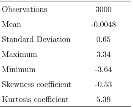
F(yt|Ft) = 0.8Φ Ã yt−0.08 p h1,t ! + 0.2Φ Ã yt−0.32 p h2,t ! (33) where h1,t = 0.003 + 0.03yt2−1+ 0.94h1,t−1 h2,t = 0.03 + 0.25yt2−1+ 0.85h2,t−1. (34) The sample size is fixed at 3000 and the conditional mean to zero. Although the second GARCH component is explosive, the model is weakly stationary because the expression given in equation (4) is equal to 0.0024. The parameters are chosen to be close to the estimates obtained for the same model using a comparable amount of real data in the empirical illus-tration described in Section 5. Table 1 provides descriptive statistics for the simulated data. The parameter values for this process clearly generate unconditional negative skewness and excess kurtosis, in addition to high persistence in the conditional variance process. This is also visible in Figure 1, which shows the sample path, the estimated kernel density, and the correlogram of the squared data.
In Table 2, we report the parameter estimates for the two component model by maximum likelihood (ML) and by Bayesian inference, using the simulated data. The ML estimator is obtained by maximizing the natural logarithm of (6) taking into account the restrictions on the component probabilities. The standard errors are obtained from the Hessian matrix evaluated at the ML estimates. The Bayesian results are the posterior means and standard
0 250 500 750 1000 1250 1500 1750 2000 2250 2500 2750 3000 −3 −2 −1 0 1 2 3
(a) Simulated data
−5 −4 −3 −2 −1 0 1 2 3 4 5 0.1 0.2 0.3 0.4 0.5 0.6 0.7
(b) Kernel density of the data
0 5 10 15 20 25 30 35 40 45 50 0.1 0.2 0.3 0.4 0.5 0.6 0.7 0.8 0.9 1.0
(c) Correlogram of squared data
Figure 1: Simulated data for the Gaussian two component mixture GARCH(1,1) model de-fined in (33)-(34).
Table 1: Descriptive statistics - simulated data Observations 3000 Mean -0.0048 Standard Deviation 0.65 Maximum 3.34 Minimum -3.64 Skewness coefficient -0.53 Kurtosis coefficient 5.39 Statistics for the simulated data of the two component model in (33)-(34).
deviations computed using 6500 draws of which the first 500 ones are discarded to warm up the Gibbs sampler. The parametersa0k of the Dirichlet prior forπare all equal to 1, implying that the prior density ofπ1 is uniform on (0,1). The prior densities for the other parameters are all independent and uniform on finite ranges, chosen to be wide enough not to truncate the posterior density but narrow enough not to waste computational time.
We see from Table 2 that the parameters estimates for both estimation methods are close to each other and of the same order of magnitude as the true values. Generally speaking, we also notice that the bias and the variance of the Bayes estimates are somewhat smaller, although some care has to be taken since the table contains only results for one simulated data set. We did a more detailed analysis of these estimators by running a Monte Carlo study, the results of which are reported in (Bauwens and Rombouts 2006), and it turns out that the smaller bias and variance for the Bayes estimator indeed are confirmed.
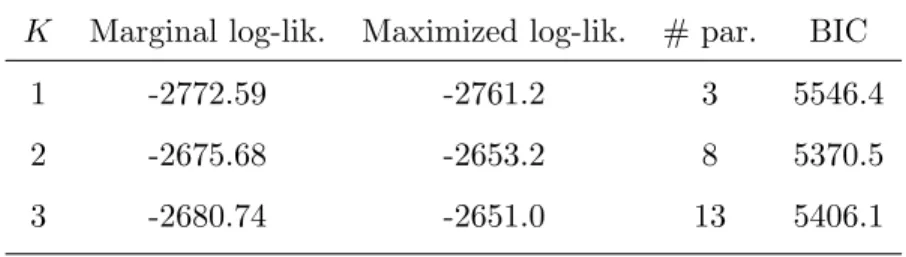
In Table 3, we report the marginal likelihood values, see Section 3.6, for the one, two and three component model. As expected, the marginal likelihood is maximized for the two component model since this is the true data generating process. To compare with the marginal likelihood, we also compute the Bayesian information criterion (BIC), defined as
−2L( ˆΨ|y)+klog(T), using the maximum likelihood estimator ˆΨ. Again, the two component model is preferred because it minimizes the BIC.
Table 2: Estimation results - simulated data
DGP MLE Bayes
estimate std error mean std dev π1 0.8 0.79824 0.040065 0.76908 0.046114 µ1 0.08 0.088729 0.011766 0.084313 0.0087951 ω1 0.003 0.0042042 0.0017198 0.0043303 0.0015511 α1 0.03 0.054952 0.0092736 0.054893 0.0081617 β1 0.94 0.89565 0.016395 0.89236 0.015149 ω2 0.03 0.019888 0.010659 0.024543 0.0094535 α2 0.25 0.18725 0.056536 0.19938 0.0494 β2 0.85 0.89226 0.027749 0.88094 0.025564 Results for two component mixture GARCH(1,1) model in (33)-(34).
Table 3: Model choice criteria - simulated data
K Marginal log-lik. Maximized log-lik. # par. BIC
1 -2772.59 -2761.2 3 5546.4
2 -2675.68 -2653.2 8 5370.5
3 -2680.74 -2651.0 13 5406.1
K is the number of components of the Gaussian mixture GARCH(1,1) model.
model performs well. In the next section we apply the model to a real dataset.
5
Application to S&P500 data
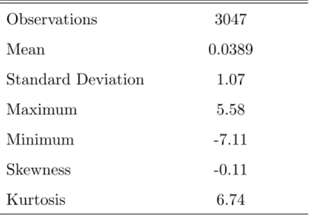
We fit the two component mixture model to daily S&P500 percentage return data from 01/03/1994 to 09/06/2005 (3047 observations). Descriptive statistics are given in Table 4. Figure 2 displays the sample path, estimated kernel density for the data and the correlogram for the squared data. It is clear from this that excess kurtosis and volatility clustering are present in the data. We analyzed whether a dynamic specification for the conditional mean is necessary and we found evidence for an autoregressive model of order three. The data are filtered for these effects in the rest of the empirical application.
Table 4: Descriptive statistics - S&P 500 returns
Observations 3047 Mean 0.0389 Standard Deviation 1.07 Maximum 5.58 Minimum -7.11 Skewness -0.11 Kurtosis 6.74
Statistics for S&P500 percentage daily returns from 01/03/1994 to 09/06/2005.
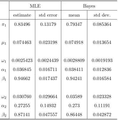
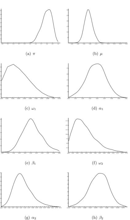
The ML estimates and the Bayes’ first two marginal posterior moments are given in Table 5. The parameters ak0 of the Dirichlet prior for π are all equal to 1 like in the simulation example. The prior densities for the other parameters are all independent and uniform on finite ranges given by 0.0001< ω1 <0.0097, 0.0005< α1 <0.08, 0.89< β1 <0.99, 0.001< ω2 < 0.13, 0.0001 < α2 < 0.73, 0.73 < β2 < 0.99. These values are the bounds used in the griddy-Gibbs sampler part of the algorithm described in Section 3.4. The posterior marginal distributions for all the parameters are given in Figure 3. The x-axes for the GARCH parameters are the prior intervals reported above. Note that the posterior marginals for ω1
0 250 500 750 1000 1250 1500 1750 2000 2250 2500 2750 3000 −6 −4 −2 0 2 4
(a) S&P 500 returns
−5 −4 −3 −2 −1 0 1 2 3 4 5 0.1 0.2 0.3 0.4 0.5
(b) Kernel density of the data
0 5 10 15 20 25 30 35 40 45 50 0.1 0.2 0.3 0.4 0.5 0.6 0.7 0.8 0.9 1.0
(c) Correlogram of squared data Figure 2: S&P 500 graphs
andω2 are somewhat truncated at zero given that they are restricted to be positive.
From Table 5, we conclude that the parameter estimates are close to each other but that the posterior standard deviations (std dev.) are smaller than the ML standard errors (std error). The latter are computed from the Hessian matrix evaluated at the ML estimates. The estimated probability is about 0.8 for the first component which is driven by a persistent α1 +β1 = 0.98 GARCH process. The second component of the mixture has a conditional variance process whereα2+β2= 1.14 with a probability of about 0.2.
Table 5: Estimation results - S&P 500
MLE Bayes
estimate std error mean std dev. π1 0.83496 0.13179 0.79347 0.085364 µ1 0.074463 0.023198 0.074918 0.013654 ω1 0.0025423 0.0024439 0.0028809 0.0019193 α1 0.036845 0.016711 0.038411 0.012836 β1 0.94662 0.017437 0.94241 0.016584 ω2 0.030760 0.029664 0.03589 0.023328 α2 0.27255 0.14932 0.273 0.11191 β2 0.87141 0.047557 0.86448 0.042872 Results for two component Gaussian mixture GARCH(1,1) model.
Figure 4 displays convergence plots for all the parameters. The convergence statistics for a parameterρ are computed as follows:
CSt= ¡1 t Pt n=1ρn ¢ −µρ σρ , (35)
whereµρandσρare the empirical mean and standard deviation, respectively, of theN draws ρ1, ρ2, . . . , ρN. If the sampler converges, the graph ofCSt againsttshould converge smoothly
0.0 0.1 0.2 0.3 0.4 0.5 0.6 0.7 0.8 0.9 1.0 0.5 1.0 1.5 2.0 2.5 3.0 3.5 4.0 (a) π 0.02 0.04 0.06 0.08 0.10 0.12 0.14 0.16 0.18 0.20 5 10 15 20 25 30 (b) µ 0.000 0.001 0.002 0.003 0.004 0.005 0.006 0.007 0.008 0.009 0.010 25 50 75 100 125 150 175 (c)ω1 0.00 0.01 0.02 0.03 0.04 0.05 0.06 0.07 0.08 5 10 15 20 25 (d) α1 0.89 0.90 0.91 0.92 0.93 0.94 0.95 0.96 0.97 0.98 0.99 5 10 15 20 25 (e)β1 0.00 0.01 0.02 0.03 0.04 0.05 0.06 0.07 0.08 0.09 0.10 0.11 0.12 0.13 2.5 5.0 7.5 10.0 12.5 15.0 17.5 (f) ω2 0.00 0.050.10 0.15 0.20 0.25 0.300.35 0.40 0.45 0.50 0.550.60 0.65 0.70 0.75 0.5 1.0 1.5 2.0 2.5 3.0 3.5 4.0 (g)α2 0.725 0.750 0.775 0.800 0.825 0.850 0.875 0.900 0.925 0.950 0.975 1 2 3 4 5 6 7 8 9 (h) β2
Figure 3: Posterior densities (kernel estimates from Gibbs output) for two component Gaus-sian mixture GARCH(1,1) model.
to zero. One can see from Figure 4 that convergence is indeed achieved for all the parameters. 500 1000 1500 2000 2500 3000 3500 4000 4500 5000 5500 6000 −1.00 −0.75 −0.50 −0.25 0.00 0.25 0.50 (a) π 500 1000 1500 2000 2500 3000 3500 4000 4500 5000 5500 6000 −0.4 −0.3 −0.2 −0.1 0.0 0.1 0.2 0.3 0.4 0.5 (b) µ 500 1000 1500 2000 2500 3000 3500 4000 4500 5000 5500 6000 −0.6 −0.4 −0.2 0.0 0.2 0.4 (c)ω1 500 1000 1500 2000 2500 3000 3500 4000 4500 5000 5500 6000 −1.00 −0.75 −0.50 −0.25 0.00 0.25 0.50 (d) α1 500 1000 1500 2000 2500 3000 3500 4000 4500 5000 5500 6000 −0.4 −0.2 0.0 0.2 0.4 0.6 0.8 (e)β1 500 1000 1500 2000 2500 3000 3500 4000 4500 5000 5500 6000 −0.4 −0.3 −0.2 −0.1 0.0 0.1 0.2 0.3 0.4 0.5 (f) ω2 500 1000 1500 2000 2500 3000 3500 4000 4500 5000 5500 6000 −0.5 −0.4 −0.3 −0.2 −0.1 0.0 0.1 0.2 0.3 0.4 0.5 (g)α2 500 1000 1500 2000 2500 3000 3500 4000 4500 5000 5500 6000 −0.4 −0.3 −0.2 −0.1 0.0 0.1 0.2 0.3 0.4 0.5 (h) β2
Figure 4: Convergence plots of Gibbs estimates of posterior means
As a comparison, we also estimate the one-component mixture model, i.e. the conventional GARCH(1,1) model. The maximum likelihood estimates and the Bayes’ first two marginal posterior moments are given in Table 6. The process looks like highly persistent, given that α1 +β1 is estimated as 0.996. This may be interpreted as a compromise between the less
persistent and explosive components of the mixture model. We obtain a similar result when we estimate the GARCH(1,1) model with the data simulated from the two component mixture of Section 4. Thus the observation that a quasi-integrated GARCH model (ˆα1+ ˆβ1 ≈1) is obtained in many empirical results can be explained by a lack of flexibility of this model.
Table 6: Estimation results (one component) - S&P 500
MLE Bayes
estimate std dev. mean std error ω1 0.0054295 0.0019993 0.0057050 0.001763 α1 0.062177 0.0082521 0.063294 0.0079359 β1 0.93494 0.0085043 0.93373 0.008198 Resulst for Gaussian GARCH(1,1) model.
in Table 7, we report the marginal likelihood and the BIC values for the one and two component models. The results indicate a strong preference for the two component model.
Table 7: Model choice criteria - S&P500 data
K Marginal log-lik. Maximized log-lik. # par. BIC
1 -4139.13 -4127.1 3 8278.2
2 -4090.87 -4071.0 8 8206.1
K is the number of components of the Gaussian mixture GARCH(1,1) model.
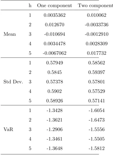
As for any time series model, prediction is essential. As we explained in Section 3.5 Bayesian inference allows to obtain predictive densities that by construction incorporate pa-rameter uncertainty. Furthermore, they can be easily computed together with the Gibbs sampler for the model parameters. We calculate predictive densities out of sample for a hori-zon up to five days, that for September 7, 2005 until September 11, 2005. Kernel density estimates for the predictive densities are given in Figure 5. The dotted line represents the two component model, the solid line represents the one component model. Eyeballing Figure
Table 8: Features of predictive densities
h One component Two components
1 0.0035362 0.010062 2 0.012670 -0.0033736 Mean 3 -0.010694 -0.0012910 4 0.0034478 0.0028309 5 -0.0067062 0.017732 1 0.57949 0.58562 2 0.5845 0.59397 Std Dev. 3 0.57378 0.57801 4 0.5902 0.57529 5 0.58926 0.57141 1 -1.3428 -1.6054 2 -1.3621 -1.6473 VaR 3 -1.2906 -1.5556 4 -1.3461 -1.5505 5 -1.3648 -1.5812
his the post-sample prediction horizon. VaR is the 5 percent value-at-risk quantile.
5, we see that the left tail of the predictive densities are fatter for the two component model compared to the simple GARCH model.
In Table 8 we give the mean, standard deviation and value-at-risk at 5 percent (VaR) for the five days. Because of the fatter left tail in the two component model, the VaR is smaller than for the one component model.
6
Conclusion
We have shown how a certain type of mixture GARCH model can be estimated by Bayesian inference. ML estimation is typically not easy because of the complexity of the likelihood
−4 −3 −2 −1 0 1 2 3 4 0.1 0.2 0.3 0.4 0.5 0.6 0.7 (a) T+1 −4 −3 −2 −1 0 1 2 3 4 0.1 0.2 0.3 0.4 0.5 0.6 0.7 (b) T+2 −4 −3 −2 −1 0 1 2 3 4 0.1 0.2 0.3 0.4 0.5 0.6 0.7 (c) T+3 −4 −3 −2 −1 0 1 2 3 4 0.1 0.2 0.3 0.4 0.5 0.6 0.7 (d) T+4 −4 −3 −2 −1 0 1 2 3 4 0.1 0.2 0.3 0.4 0.5 0.6 0.7 (e) T+5
Figure 5: Kernel density estimates of predictive densities from September 7, 2005 to Septem-ber 11, 2005. The dotted line represents the two component model, the solid line represents the one component model.
function. In Bayesian estimation, this is taken care of by enlarging the parameter space with state variables, so that a Gibbs sampling algorithm is easy to implement. Despite a higher computing time, the Bayesian solution is more reliable since estimation does not fail, while this may happen in MLE. Moreover, as we show in Section 3, the Gibbs algorithm can be extended to include the computation of predictive densities, which takes care of estimation uncertainty. Prediction in the ML approach is typically done by conditioning on the ML estimate and therefore ignores estimation uncertainty.
Bayesian estimation of other types of mixture GARCH models, including multivariate models, can probably be handled in a similar way as in this paper. Such extensions are on our research agenbda.
References
Alexander, C., and E. Lazar (2004): “Normal Mixture GARCH(1,1),” forthcoming in
Journal of Applied Econometrics.
Bauwens, L., C. Bos, R. van Oest,andH. van Dijk(2004): “Adaptive radial-based di-rection sampling: a class of flexible and robust Monte Carlo integration methods,”Journal of Econometrics, 123/2, 201–225.
Bauwens, L., M. Lubrano, and J. Richard (1999): Bayesian Inference in Dynamic Econometric Models. Oxford University Press, Oxford.
Bauwens, L., and J. Rombouts (2006): “A comparison of estimators for the mixed con-ditional heteroskedasticity model,” forthcoming CORE DP.
Bollerslev, T.(1986): “Generalized Autoregressive Conditional Heteroskedasticity,” Jour-nal of Econometrics, 31, 307–327.
Bollerslev, T., R. Engle, and D. Nelson (1994): “ARCH Models,” in Handbook of Econometrics, ed. by R. Engle, andD. McFadden, chap. 4, pp. 2959–3038. North Holland Press, Amsterdam.
Dempster, A., N. Laird, and D. Rubin (1977): “Maximum Likelihood for Incomplete Data via the EM Algorithm (with discussion),” Journal of the Royal Statistical Society Series B, 39, 1–38.
Haas, M., S. Mittnik, and M. Paolella (2004a): “Mixed Normal Conditional Het-eroskedasticity,”Journal of Financial Econometrics, 2, 211–250.
(2004b): “A New Approach to Markov-Switching GARCH Models,” Journal of Financial Econometrics, 2, 493–530.
Kass, R., and A. Raftery (1995): “Bayes Factors,” Journal of the American Statistical Association, 90, 773–795.
Marin, J., K. Mengersen,and C. Robert (2005): Bayesian Modelling and Inference on Mixtures of Distributions, Handbook of Statistics 25. D. Dey and C.R. Rao (eds), Elsevier-Sciences.
McLachlan, G., and D. Peel (2000): Finite Mixture Models. Wiley Interscience, New York.
Nelson, D. (1991): “Conditional Heteroskedasticity in Asset Returns: a New Approach,”
Econometrica, 59, 349–370.
Richardson, S., and P. Green (1997): “On Bayesian Analysis of Mixtures with an Un-known Number of Components,” Journal of the Royal Statistical Society, Series B, 59, 731–792.
Tanner, M., and W. Wong (1987): “The calculation of posterior distributions by data augmentation,”Journal of the American Statistical Association, 82, 528–540.
Tierney, L., and J. Kadane (1986): “Accurate Approximations for Posterior Moments and Marginal Densities,”Journal of the American Statistical Association, 81, 82–86.
Wilks, S.(1962): Mathematical Statistics. Wiley, New York.
Wong, C., and W. Li(2000): “On a Mixture Autoregressive Model,” Journal of the Royal Statistical Society, Series B, 62, 95–115.
(2001): “On a Mixture Autoregressive Conditional Heteroscedastic Model,”Journal of the American Statistical Association, 96, 982–995s.