Portland State University
PDXScholar
Dissertations and Theses Dissertations and Theses
Fall 10-27-2014
Analog Implicit Functional Testing using Supervised Machine
Learning
Neerja Pramod Bawaskar
Portland State UniversityLet us know how access to this document benefits you.
Follow this and additional works at:http://pdxscholar.library.pdx.edu/open_access_etds Part of theElectrical and Computer Engineering Commons
Recommended Citation
Bawaskar, Neerja Pramod, "Analog Implicit Functional Testing using Supervised Machine Learning" (2014).Dissertations and Theses.
Paper 2099. 10.15760/etd.2097
Analog Implicit Functional Testing using Supervised Machine Learning
by
Neerja Pramod Bawaskar
A thesis submitted in partial fulfillment of the requirements for the degree of
Master of Science in
Electrical and Computer Engineering
Thesis Committee: W. Robert Daasch, Chair
C. Glenn Shirley Mark Faust
Portland State University 2014
Abstract
Testing analog circuits is more difficult than digital circuits. The reasons for this difficulty include continuous time and amplitude signals, lack of well-accepted test-ing techniques and time and cost required for its realization. The traditional method for testing analog circuits involves measuring all the performance param-eters and comparing the measured paramparam-eters with the limits of the data-sheet specifications. Because of the large number of data-sheet specifications, the test generation and application requires long test times and expensive test equipment.
This thesis proposes an implicit functional testing technique for analog circuits that can be easily implemented in BIST circuitry. The proposed technique does not require measuring data-sheet performance parameters. To simplify the testing only time domain digital input is required. For each circuit under test (CUT) a cross-covariance signature is computed from the test input and CUT’s output. The proposed method requires a training sample of the CUT to be binned to the data-sheet specifications. The binned CUT sample cross-covariance signatures are mapped with a supervised machine learning classifier. For each bin, the classifiers select unique sub-sets of the cross-covariance signature. The trained classifier is then used to bin newly manufactured copies of the CUT.
The proposed technique is evaluated on synthetic data generated from the Monte Carlo simulation of the nominal circuit. Results show the machine learning clas-sifier must be chosen to match the imbalanced bin populations common in analog circuit testing. For sample sizes of 700+ and training for individual bins, classifier
Acknowledgements
I would like to express my deepest gratitude to all those people who have directly or indirectly helped me in the completion of my thesis. I would foremost like to thank my research advisor Dr.Robert Daasch for being such a wonderful mentor. His deep insight and research experience in the field of IC testing and our one-on-one and group meetings have given me invaluable knowledge and also helped me develop my presentation skills. Without his guidance, patience and motivation this thesis would not have been possible. I would also like to thank Dr.Glenn Shirley for his valuable feedback and meticulous suggestions for my work. Special thanks to Prof. Mark Faust for agreeing to serve on my thesis committee.
I am deeply grateful to all my ICDT colleagues for their support and motivation throughout my thesis program. Special thanks to Yushan, Nagarjun and Chris who helped me in tough times. Advice and warm encouragement from Dr. John Acken has been a great help to me. Special thanks to my dear friends Nikita, Madhura and Ketaki for the continued friendship, discussions and all the happy times we spent together.
Last but not the least, my deepest gratitude to my family here in US and back in my home town. I am eternally grateful to my parents and younger sister Anuja for being such a wonderful and loving support throughout my life. I cannot thank Rohan enough for his constant motivation, support and patience for putting up with my grumpiness at times.
Contents
Abstract i
Acknowledgments ii
List of Tables vii
List of Figures viii
1 Introduction 1
1.1 Brief description of the thesis . . . 1
1.2 Introduction to IC Test . . . 1
1.3 Problem Statement . . . 2
1.4 Proposed Solution . . . 4
1.5 Contribution of Thesis . . . 4
1.6 Organization of Thesis . . . 5
2 Background and Previous Work 6 2.1 Cross covariance . . . 6
2.2 Performance Space Testing . . . 7
2.3 Signature Space Testing . . . 8
2.4 Monte Carlo method . . . 8
2.5 Supervised machine learning . . . 10
2.5.1 AdaBoost algorithm . . . 10
2.6 Previous Work . . . 15
3 Strategy to evaluate implicit functional testing 19 3.1 Circuit Under Test . . . 19
3.2 Synthetic process variation using Monte Carlo method . . . 20
3.3 Constructing the signature . . . 20
3.4 Mapping performance space to signature space . . . 21
3.5 Training a strong classifier . . . 22
4 Results for evaluating IFT using Monte Carlo data 26 4.1 Infrastructure for constructing signature . . . 26
4.1.1 Circuit Under Test (CUT) . . . 26
4.1.2 Synthetic Process Variation . . . 27
4.1.3 Waveform Generator . . . 28
4.1.4 Cross covariance as a signature . . . 34
4.1.5 Mapping performance parameters to the signature . . . 37
4.2 Classifier training and testing . . . 40
4.2.1 Classifier details . . . 41
4.2.2 Results table description . . . 42
4.2.3 Pass-gain fail only classifier . . . 44
4.2.4 Pass-gain-bandwidth fail only classifier . . . 44
4.2.5 Pass-both fail classifier . . . 45
4.2.6 Summary of over-kill and test-escape for the trained classifiers 47 4.2.7 Pass-all fails combined classifier . . . 49
4.2.8 Pass, gain fail only, gbw fail only, both fail classifier . . . 49
5 Conclusion and Recommendations for Future Work 55
5.1 Conclusion . . . 55 5.2 Recommendations for future work . . . 56
List of Tables
4.1 Transistor dimensions of the OTA . . . 27
4.2 Functional and non-functional inputs . . . 31
4.3 Input test patterns . . . 32
4.4 Sampling rates for input patterns . . . 32
4.5 Signature set . . . 37
4.6 Limits set . . . 37
4.7 Data table . . . 39
4.8 Subsets of signature used by the trained classifiers . . . 42
4.9 Pass-gain fail only classifier results. . . 44
4.10 Cross-covariances used by pass-gain fail only classifier. . . 44
4.11 Pass-gain-bandwidth fail only classifier results. . . 44
4.12 Cross-covariance used by pass-gain-bandwidth fail only classifier. . . 44
4.13 Pass-both fail classifier results. . . 45
4.14 Cross-covariance used by pass-both fail classifier. . . 45
4.15 Testing both fail instances on pass-gain classifier . . . 45
4.16 Testing both fail instances on pass-gain-bandwidth fail only classifier. 45 4.17 Over-kills for trained classifiers . . . 47
4.18 Test-escapes for the trained classifiers. . . 48
4.19 Pass-all fails combined classifier results. . . 49
4.20 Cross-covariance used by pass-all fails combined classifier. . . 49
4.22 Cross-covariance used by pass,gain fail only, gbw fail only, both fail classifiers. . . 51 4.23 Ideal and Noisy classifier results. . . 53 4.24 Cross-covariance used by ideal and noisy classifier. . . 53
List of Figures
1.1 Reduced accessibility of analog signals in mixed signal SOC . . . 3
2.1 AdaBoost pseudo-code . . . 11
2.2 Traning data for toy example . . . 12
2.3 Hypothesis by weak learners . . . 13
2.4 Final hypothesis . . . 14
2.5 RUSBoost Pseudocode . . . 15
2.6 Analog test flow . . . 16
2.7 LTI system . . . 18
3.1 Embedding CUT in data converters . . . 19
3.2 Strategy for constructing the signature . . . 21
3.3 Mapping performance space to signature space . . . 22
3.4 Weak learner . . . 23
3.5 Strong classifier . . . 24
3.6 Strategy for testing analog circuits . . . 25
4.1 Schematic of OTA . . . 27
4.2 Waveform generator . . . 29
4.3 Schematic of 10-bit DAC . . . 30
4.4 Input test patterns in time and frequecy domain . . . 33
4.5 Sampling inputs and outputs . . . 34
4.6 Inputs, outputs and cross-covariance . . . 36
4.8 Imbalanced data . . . 40
4.9 Strong classfier using 300 weak learners . . . 41
4.10 Zoomed performance plot . . . 48
4.11 Weak learners for multilabel classifiers . . . 50
4.12 Sampling digital input . . . 52
Chapter 1 Introduction
1.1 Brief description of the thesis
This thesis proposes an implicit functional testing technique for analog circuits. The technique involves classification using a set of signatures without measuring all the performance parameters to test analog circuits. A classifier is trained selecting the subset of the signature by a supervised machine learning algorithm. The trained classifier is used to bin new copies of the circuit as pass or fail.
1.2 Introduction to IC Test
Testing integrated circuits to differentiate between faulty and fault-free circuits basically involves three steps- generating a suitable test input pattern, capturing the response of the circuit and comparing the response with the expected response. If the captured and expected responses match, the circuit is classified as fault-free else it is classified as faulty. For digital circuits, the expected response is a unique value. Whereas for analog circuits, the expected response can have a wide range of accepted values. In analog testing, if the difference between the responses is greater than a predetermined tolerance limit the circuit is considered as faulty else it is considered as fault-free. The predetermined tolerance limit is set depending on factors such as process variation and measurement accuracies [1].
Faults in analog circuits can be classified as catastrophic faults or parametric faults [2]. Catastrophic faults are hard faults such as short circuit or open circuit that
occur in gate-level interconnects. These faults can also occur anywhere in the topology of the circuit resulting in dead-on-arrival circuits (DOA). Parametric faults are soft faults that cause the performance parameters of the circuit to fall outside the acceptable tolerance limits. The shift in the performance parameters can cause the circuit to fail to meet the data-sheet specifications.
In semiconductor test, the circuit fails in test even if a single fault is detected. A fault-free circuit passes in test since all the requirements are met. An ideal test passes all fault-free circuits and fails all the faulty ones. However, in practice, a faulty circuit maybe classified as free resulting in a test escape and a fault-free circuit maybe classified as faulty resulting in over-kill. The goal of the test is to minimize the percentage of test escapes and over-kills at an acceptable cost.
An end use defect level should be between 10 to 1000 defective parts per million (DPPM) for analog circuits for maintaining the quality of the product [3]. For example, the dataset of a mixed signal automotive product consists of 6800 dies per wafer. The number of passing and failing dies in test is around 6560 and 240 respectively. This is an example of imbalanced data where there is a significantly dominant population group and a minority population group.
1.3 Problem Statement
There is a need for new techniques to bin analog circuits as pass or fail. Analog circuits are integrated along with digital and mixed-signal circuits on the same substrate to reduce circuit packaging and assembly costs [1]. Integration on the same substrate results in reduced controllability and observability of input and
in Figure 1.1.
Figure 1.1: The observability of analog signals is reduced in mixed-signal SOC. Testing analog modules in mixed-signal SOC becomes difficult and expensive [4]
.
Testing analog circuits is more difficult than digital circuits. There are several sources for the difficulty such as continuous amplitude and time signals, lack of broadly-applicable testing techniques, and the time and cost required for testing analog circuits [4]. Conventional methods for testing analog circuits measure the performance parameters and compare the measured response with the tolerance limit of the design specifications. But the number of design specifications for an analog circuit is large. Measuring the performance parameters for all such specifica-tions requires complex test equipment as well as long test application time. Analog signals are multi-valued signals because a wide range of values about a nominal value is acceptable [1]. Generating input test patterns in the frequency domain and analyzing the responses of the analog circuits requires expensive equipment. In contrast to digital testing, analog testing determines whether the output response values are within the acceptable tolerance limit rather than a specific value. The response is not a sequence of zeros or ones but frequency characteristics, phase
margin, current gain and so on.
The performance of analog circuits is strongly dependent on manufacturing process variation. Process variation can cause the component parameter values to deviate from the expected value by as much as 20% [1]. Proper functioning of the circuit may be affected resulting in failure to meet the performance specifications.
1.4 Proposed Solution
As a solution for the above mentioned problems, an implicit functional testing technique is proposed in this thesis . The proposed implicit functional testing technique uses a set of test signatures to bin circuits as pass or fail. The test signature is easier to compute than measuring all the performance parameters. The technique proposes digital measurements in the time domain. For testing analog circuits, time domain measurements are easier and less time consuming than frequency measurements. The analog circuit is embedded with data converters and measures the signals in digital time domain. The response of the circuits is captured and post processed to construct a signature. The signature is then mapped to the data-sheet specifications. The subsets of the signature are selected by the classifier using a supervised machine learning algorithm. The trained classifier is used to bin new copies of the circuits as pass or fail based on the signature of the circuits.
1.5 Contribution of Thesis
The main contribution of this thesis is to propose an analog testing technique similar to present digital testing techniques. The proposed technique can be easily implemented in Built In Self Test (BIST) circuitry. The method of generation
of the input test pattern and capturing the response of the CUT is analogous to digital testing. Cheng’s [5] implicit functional testing used a set of signatures rather than explicitly measuring the performance parameters to bin analog circuits as pass or fail. This thesis extends Cheng’s work by further mapping the signature to data-sheet specifications using supervised machine learning technique to bin the circuits as pass or fail.
1.6 Organization of Thesis
This thesis is organized in five chapters. The second chapter describes concepts used in this study and summarizes previous work done in the field of analog testing. The concepts are cross-covariance, performance space, signature space testing, Monte Carlo method, supervised machine learning. The strategy for testing analog circuits is proposed in Chapter 3. Results of the proposed strategy are presented in Chapter 4. Conclusions and recommendations for future work are presented in Chapter 5.
Chapter 2
Background and Previous Work
This chapter describes background concepts such as cross-covariance, performance space testing, signature space testing, Monte Carlo method and supervised machine learning as well as the similar work done in the field of analog testing.
2.1 Cross covariance
A linear time invariant(LTI) system is fully characterized by its impulse response function [5]. The impulse response can be constructed from the cross-covariance between the input and the output of the LTI system. Cross-covariance is a measure of similarity of two signals as a function of time-shift between them. The cross-covariance of two random vectors x and y is given as,
cov(x, y) =E[(x−µx)(y−µy)] (2.1)
where E is the expectation operator, µx and µy are the mean scalars subtracted
from the vectors that contain the expected values of x and y [6].
In this thesis, the cross-covariance is calculated using the Matlab statistics toolbox [7]. Consider two random vectors x and y of length N with sample means of µx,
and µy, respectively. The cross-covariance vector φxy has length m=1...2N-1 and
φxy(m)= N−|m|−1 P n=0 xn+m− N1 N−1 P i=0 xi yn−N1 N−1 P i=0 yi m ≥0 φyx(−m) m <0 (2.2)
In order to ease the comparison between cross-covariances for different input and outputs, normalization at zero lag is selected.
φxy(m)= E[(x−µx)(y−µy)] E[xn, yn] = E[(x−µx)(y−µy)] φxy(0) (2.3) At a particular offset m,
φxy(m)= 1 indicates that the two vectors are identical.
φxy(m)= 0 indicates that there is no similarity between the two vectors.
φxy(m)= -1 indicates that the vectors are identical but out of phase.
2.2 Performance Space Testing
Performance space testing involves measuring the data-sheet specifications that need to be satisfied by the circuit. The circuit is binned as either pass or fail by comparing its measured performance parameters with the data-sheet specifications. The wide range of data-sheet specifications leads to difficulty in the test generation and application. Testing in performance space, called explicit functional testing, establishes that the manufactured circuits lie within the ranges of the data-sheet specifications. To bin circuits based on the data-sheet specifications, the input test patterns must be functional. Since the data-sheet specifications are different for different analog circuits, testing in performance space can be used to test only a certain class of circuits.
2.3 Signature Space Testing
In signature space testing, the response of a circuit is captured for any given input test pattern. The captured response is post-processed to construct a signature. The signature is then used to bin analog circuits. Since the testing is not confined to data-sheet specifications in signature space, there is no restriction for the input test patterns: they can be either functional or functional. Testing with non-functional inputs is analogous to digital circuit testing where the inputs that can detect stuck-at faults are not the expected inputs during use. The signature is mapped to the data-sheet specifications to bin circuits based on their performance parameters. Another advantage of signature space testing is that it can be used to test different class of circuits. Analog circuit test in signature space is called as implicit functional testing because measuring the function of the CUT is not necessary [5].
2.4 Monte Carlo method
Monte Carlo is the most common method to simulate process variations syntheti-cally in the circuit. There are two aspects of process variation modeled by Monte Carlo: process and mismatch [8]. In process variation, all the n-type transistors are varied in the same manner and all the p-type transistors are varied in the same manner. Whereas in mismatch a n-type transistor or a p-type transistor is varied individually in a different manner. Process variation can be used to analyze the design margin of the circuit whereas mismatch variation can be used to evaluate the yield statistics of the circuit.
The compact modeling technique [9] assumes that the model parameters of the transistors vary statistically . The transistor model parameters are assumed to be normally distributed statistical variables. For example, the deviation of the pa-rameters lengthl, threshold voltagevth and oxide thicknesstox from their nominal values is given as,
Ml Mvth Mtox = g11 g12 g13 g21 g22 g23 g31 g32 g33 x1 x2 x3 ≡G x1 x2 x3 (2.4)
where x1, x2, x3 are random variables with standard normal distribution [9].
The G matrix can be properly determined to closely resemble the real device variations. The generalized form of the equation can be expressed as,
Mp1 Mp2 . . Mpm = g11 g12 ... g1M g21 g22 ... g2M . . ... . . . ... . gm1 gm2 ... gmM x1 x2 . . xM ≡G x1 x2 . . xM (2.5)
whereMpi is the deviation of the ith compact model parameters, G is the
In this thesis, TSMC 90nm compact modeling technique is used [26]. The TSMC 90nm compact modeling technique is implemented using the general compact mod-eling technique. The Gaussian random variablesx1, x2, ..., xM achieve the
random-ization.
2.5 Supervised machine learning
Supervised machine learning trains a model from a known input data and a known response to the data in order to predict unknown response of new data. Supervised learning is split into two broad categories, namely: classification trees and regres-sion trees. Classification trees are used when categorical response values (eg. pass or fail) are required whereas regression trees are used when continuous response values are required (eg. miles of a car per gallon [10]).
A classification tree is known as a weak learner when its prediction is slightly better than random guessing [11]. A weak learner outputs a correct hypothesis only for a small fraction of the data. The classification can be improved by combining the majority vote of multiple weak learners to build a strong classifier using boosting algorithms [12]. Depending on the nature of the data, there are various boost-ing algorithms available such as AdaBoost,RUSBoost, LogitBoost, Gentle Boost, LPBoost , RobustBoost [13].
2.5.1 AdaBoost algorithm
The most common boosting algorithm used is the AdaBoost or Adaptive boost algorithm [14]. AdaBoost tweaks the subsequent weak learners depending on the instances misclassified by the previous weak learners. The pseudo-code for the
AdaBoost algorithm is shown in Figure 2.1.
Figure 2.1: The AdaBoost algorithm adaptively tweaks the weights of the in-stances misclassified by the previous weak learner. The weights are increased if the instances is misclassified and decreased if the instance is correctly classified. The weights are updated after every iteration.
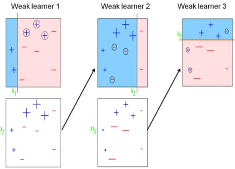
The pseudo-code is explained with the help of a simple example of boosting [?] where the aim is to train a classifier to classify any new sign as ’+’ or ’-’ . The training data is a group of five minus and five plus signs as shown in Figure 2.2. The strong classifier is trained using three weak learners (T=3). The ten instances (N) are initialized to equal weights.(Line 1 from Fig 2.1)
Figure 2.2: The training data consists of 5 instances of plus signs and 5 instances of minus signs. All the instances are initialized to equal weights.
Figure 2.3 shows that weak learner 1 outputs a hypothesis h1 (Line 3 from Fig 2.1). The error of the hypothesis of weak learner 1 is calculated (Line 4 from Fig 2.1). The weights of the instances are now updated (Line 5 from Fig 2.1). The weights of the three misclassified pluses are increased (Line 6) and the weights of the remaining correctly classified instances are decreased (Line 7 from Fig 2.1). For the next iteration (t), weak learner 2 concentrates on the misclassified instances and outputs a hypothesis h2 as shown in Figure 2.3 that correctly classifies the three pluses. So the weights of the correctly classified instances are decreased and the weights of three misclassified minus signs are increased. For the third iteration, weak learner 3 outputs a hypothesis h3 to correctly classify the three minuses.
Figure 2.3: Each weak learner outputs a hypothesis to classify the instances into two groups. The weights of the misclassified instances are increased and the weights of the correctly classified instances are decreased. The subsequent weak learner concentrates on the instances misclassified by the previous weak learner.
The final hypotheses is obtained by combining the weighted sum of the individual hypothesis (Line 8 from Fig 2.1). A strong classifier is built by combining the three weak learners as shown in Figure 2.4. Any new instance will be classified as plus or minus by taking the weighted majority vote of the weak learners.
Figure 2.4: The weighted sum of the individual hypothesis of the weak learners is combined to form the final hypothesis.
2.5.2 RUSBoost algorithm for imbalanced data
The data may not always have equal number of pass and fail instances. For such imbalanced data, the data is first sampled before applying the boosting technique. RUSBoost (Random Under Sampling) is one algorithm used for training with im-balanced data [15]. The difference between RUSBoost and AdaBoost algorithm is that the dataset is randomly under-sampled before applying the boosting technique ( Line 3 2.5) [15]. In under-sampling, the instances from the majority population group are removed until they are equal to the number of instances in the minority population group.
Figure 2.5: The figure shows the pseudo-code for RUSBoost algorithm. The Ran-dom Undersampling Boost algorithm is similar to the AdaBoost except for line 3. The instances from the majority population group are undersampled until they are equal with the minority population group. After the appropriate sampling, the boosting is done.
2.6 Previous Work
Research in testing analog circuits has received substantial attention because of the increased advancement in digital IC testing techniques and algorithms. Several testing techniques for analog circuits have been suggested in the past years as shown in the figure below.
Figure 2.6: The flowchart represents the different techniques proposed by re-searchers for testing analog circuits. Most of the proposed work has been related to explicit functional testing for analog circuits. This thesis proposes an implicit functional testing technique.
Milor [16] suggested an explicit functional testing technique using a reduced spec-ification test set to reduce the time required for testing. The reduced specspec-ification test set consisted of list of parameters such as phase margin, output swing, power dissipation, gain, output swing, slew rate. Wagner [17] suggested isolation of ana-log modules from the digital modules to apply test inputs. The bandwidth, current and voltage parameters were measured with the help of additional circuitry to test analog circuits. However, even for the reduced test set, these suggested techniques of specification based testing is cumbersome because of the range of accepted values
for analog circuits.
Kaminska [18] proposed a DFT technique to alter the structure of the circuit-under-test (CUT) during testing. The functional building blocks such as filters, PLL, amplifiers, comparators were transformed into oscillators. The oscillation frequency of the oscillator was measured and used as a signature. The tolerance limit for the oscillation frequency was obtained by the Monte Carlo analysis of the altered circuit. Altering the CUT can help detect structural faults. However, the functionality of the CUT is not tested with this technique.
Papakostas [19] and Wang [20] explored the concept of using spectrum of the power-supply current as a signature to classify analog circuits as faulty or fault-free. The analysis of the power-supply current spectrum was performed during the design stage of the circuit so that it can be used as a signature in the testing stage. This type of testing is called explicit functional testing since the mapping of the signature is done to every value in the performance space.
Bachir [21] suggested a signature space testing technique where a fault-free and faulty CUT are excited with the same test input signal. The power spectral density of the output response is used as a signature. The signature of the faulty CUT is compared with the fault-less signature to classify the CUT as faulty or fault free. The mapping of the signature is not done to the performance space, hence this testing technique is also called as explicit testing technique.
Cheng [5] first introduced implicit functional testing where the analog linear time invariant (LTI) circuit was modeled as a digital LTI circuit as shown in Figure
2.7. The impulse response function of the LTI circuit can be constructed using cross-correlation. [5]
Figure 2.7: The output random process Y is a linear tranformation of the input random process X by the LTI circuit. The cross correlation between X and Y is proportional to the impulse response h(n) [5].
The CUT was embedded between data converters during testing. The input pat-tern was generated using LFSR and applied to the CUT. The cross correlation between the input and the delayed input pattern with the output was computed. Cheng used cross correlation as a signature to classify circuits as faulty or fault-free. The limits for the signature were obtained by mapping the performance space to signature space. This thesis extends Cheng’s work [5] by using subsets of signature to train a classifier to bin circuits as pass or fail.
Chapter 3
Strategy to evaluate implicit functional testing
This chapter describes the strategy implemented for the evaluation of the proposed implicit functional testing (IFT).
3.1 Circuit Under Test
Analog signals are difficult to generate and measure during testing. In order to ease the manipulation of the analog signals, the analog circuit is treated as a digital circuit by embedding the circuit between a digital-to-analog converter and an analog-to-digital converter during testing. [5].
Figure 3.1: The analog circuit is the CUT which is embedded between data con-verters during testing. The input to the DAC is a n-bit digital signal. The analog output of the DAC is provided as an input to the analog circuit (CUT). The analog output of the circuit is converted to the n-bit digital signal using the ADC.
The analog circuit is tested using time domain digital measurements as opposed to the frequency domain measurements traditionally employed in analog test. Digital measurements are easier to implement and require simple circuitry.
3.2 Synthetic process variation using Monte Carlo method
The Monte Carlo method introduced in Chapter 2 is used to achieve the synthetic process variation of the CUT. The specified design margin takes into consideration the environmental and process variations that can affect the performance of the circuit. In order to simulate the manufacturing process variations that affect the circuit performance, the nominal circuit is simulated over a wide range of device parameters using the standard Monte Carlo method. The variation of n-type transistors is the same and the variation of the p-type transistors is the same. The synthetic process variation is achieved by the Monte Carlo simulation using the Cadence Spectre tool. The compact modeling technique implemented by TSMC is used to achieve the randomization for the model parameters.
3.3 Constructing the signature
An input test pattern to the CUT is applied through a 10-bit DAC. The response of the circuit to the input is captured. The captured response is converted to digital signal using the 10-bit ADC quantizer. There are four possible ways for sampling the input and output: digital input-digital output, analog input-analog output, analog input-digital output and digital input-analog output. Cheng [5] computed the cross-correlation of the digital input and digital output signal to construct the signature. In this thesis, the digital input-digital output as well as the analog input-digital output is sampled.
In this thesis, the cross-covariance of the input and output of the simulated in-stances is computed to construct the signature. The covariance is the cross-correlation of the mean-removed sequence. The cross-covariance is unique for each
instance. This thesis uses the cross-covariance vector as a signature to bin circuits as pass or fail. Matlab Signal Processing Toolbox is used to compute the cross covariance [22]
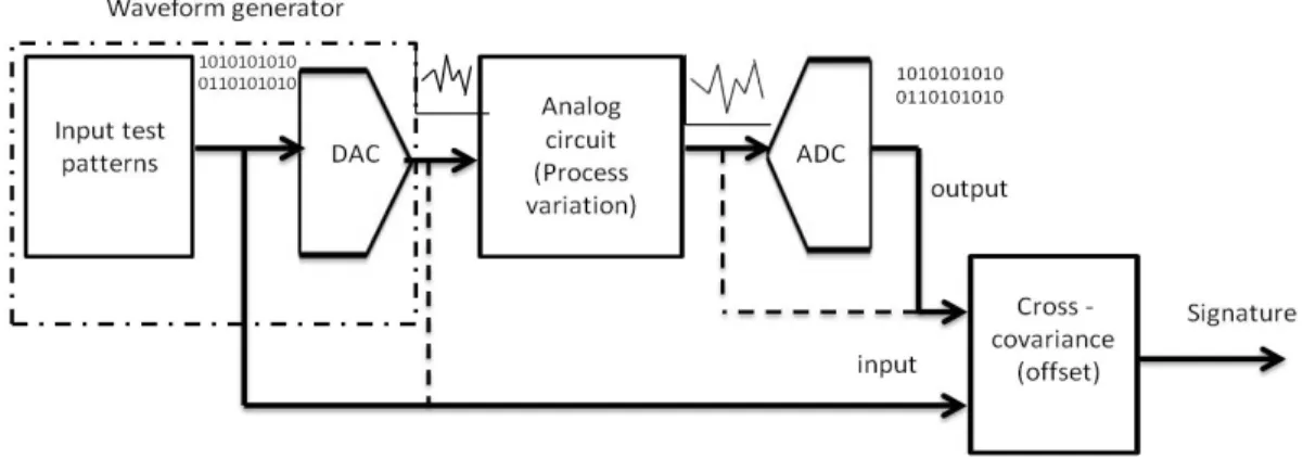
Figure 3.2: The figure shows the strategy for constructing the signature. The waveform generator is used to generate input test patterns for the analog CUT. The cross-covariance of the input and output of the Monte Carlo instances are computed. The cross-covariance vector is used as a signature.
3.4 Mapping performance space to signature space
When testing in performance space, the circuit response is compared directly to the data-sheet specifications and classified as pass or fail. Figure 3.3a shows an example where performance space is a one-dimensional space. If an instance’s response lies within the data-sheet limits, it is classified as pass else it is classified as fail. However, testing in signature space requires mapping the signature to data-sheet specification because cross-covariance is not a deciding factor to bin a circuit as pass or fail. Every instance in performance space can be mapped to signature space by either simulation or regression so instances in performance space can lie anywhere in the two-dimensional signature space as shown in Figure 3.3b. In
this thesis, the cross-covariance at two different offsets forms the two-dimensional signature space.
Figure 3.3: The figure shows the mapping between performance space and signa-ture space. Depending on the data-sheet specifications, an instance in the perfor-mance space is classified as either pass or fail. Every instance in the perforperfor-mance space is mapped to an instance in the signature space. The cross-covariance forms the two-dimensional signature space. The axes in the signature space are cross-covariances at two different offsets. The boundaries in the signature space are obtained by using supervised machine learning.
Even though the signature space is a high dimensional space, the testing is easier to implement in signature space as discussed in Chapter 2. The mapped signature is used to bin circuits as pass or fail. The constructed signature is the cross covariance along with the corresponding bin from the performance space.
3.5 Training a strong classifier
The concept of supervised machine learning illustrated in Chapter 2 is described in this section. The classifiers are trained using Matlab statistics toolbox version R2014a. The tolerance limits for the mapped signature are obtained by training
a strong classifier using supervised machine learning. A strong classifier is built with the help of supervised machine learning to bin any new instance as pass or fail. The strong classifier is built by combining the majority votes of the number of weak learners. As mentioned in Chapter 2, weak learners are the classifiers that perform slightly better than random guessing. Figure 3.4 shows a weak learner. The weak learner with the help of a weak learning algorithm classifies the instances into two bins namely pass and fail. The misclassification error is slightly less than 50%.
Figure 3.4: A weak learner. The weak learner classifies the pass and fail instances with a misclassification error slightly less than 50%. The fail instances may be misclassified as pass leading to test-escapes (TE) and the pass instances may be misclassified as fail leading to over-kills (OK). The percentage of the test-escapes and over-kills is dependent on the population of the data.
To reduce the misclassification error, the weighted majority vote of the weak learn-ers is combined to build a strong classifier as seen in Figure 3.5. In real test data, the number of pass instances is more than the number of fail instances. The imbal-ance in the data can lead to under-training of the fail instimbal-ances and over-training of the pass instances. In this case the classifier outputs more number of test es-capes than over-kill units. The increase in the number of test eses-capes will result in shipping the faulty circuits to the customer. To avoid this situation, the pass instances are under-sampled until the number of pass and fail instances is equal
before applying the boosting technique.
Figure 3.5: Training a strong classifier by combining weak learners (WL) with the help of supervised machine learning algorithm. The number of test-escapes (TE) and over-kills (OK) is reduced after appropriate sampling of the data and boosting of the weak learners .
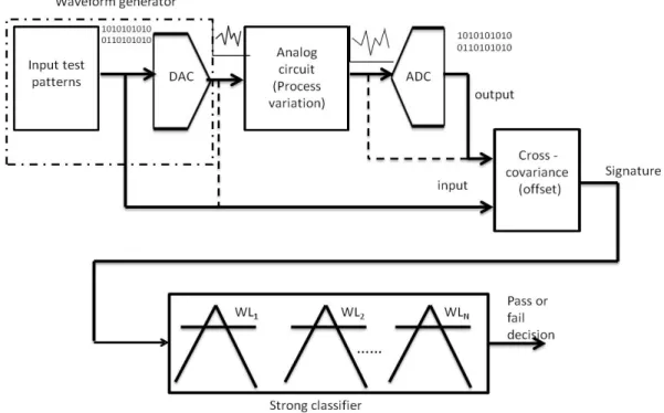
The trained strong classifier is used to bin new copies of the circuit. Based on the signature of a circuit, the classifier outputs a result whether an instance is pass or fail. The following figure shows the entire strategy for testing analog circuits as proposed in this work.
Figure 3.6: The figure shows the complete strategy to evaluate the proposed im-plicit functional testing for analog circuits. The constructed signature is used to train a strong classifier. The trained classifier uses subsets of signature to bin copies of the circuits as pass or fail.
Chapter 4
Results for evaluating IFT using Monte Carlo data
This chapter is organized in two main sections. The first section describes the infrastructure for constructing the signature. The second section demonstrates the results obtained by training the classifier with the constructed signature.
4.1 Infrastructure for constructing signature
This section is organized in four subsections. The first subsection describes the Circuit Under Test (CUT) designed to demonstrate the results for the proposed strategy. Subsection 2 explains the synthetic process variation done using Monte Carlo simulation. Subsection 3 describes the input test patterns generated by the waveform generator. The construction of the signature is described in the last subsection.
4.1.1 Circuit Under Test (CUT)
The Circuit Under Test (CUT) chosen for this work is an analog amplifier built using an operational transconductance amplifier (OTA). The OTA is designed in 90nm technology and is a common analog building block. The OTA has nominal gain of 4 and bandwidth of 300 kHz at typical operating conditions (Vdd=0.9V,27◦C). The data-sheet input operating range is 400mV- 600mV. Fig-ure 4.1 shows the schematic of the OTA and Table 4.1 provides the dimensions of the transistors in the OTA.
Figure 4.1: The figure shows the schematic of the OTA designed in 90nm technol-ogy. The input test pattern is applied to the inverting input VIN−.
Transistor Type Width (nanometer) Length (nanometer)
MP1 PMOS 1000 240 MP2 PMOS 1000 240 MP3 PMOS 1000 240 MN1 NMOS 1000 200 MN2 NMOS 1000 200 MN3 NMOS 90 200 MN4 NMOS 1000 200 MN5 NMOS 1000 200
Table 4.1: Transistor dimensions of the OTA
4.1.2 Synthetic Process Variation
The Monte Carlo method is used to simulate the manufacturing process variations of the OTA. The synthetic process variation of the transistor model parameters in the OTA is done using the compact modeling technique implemented by TSMC as discussed in Chapter 2. The Monte Carlo method is used to generate 1500
instances with the synthetic process variations. Each instance is indexed by four Monte Carlo parameters: random1, random2, random3, random4. The four Monte Carlo parameters are varied independently with Gaussian distribution having mean (µ) equal to 0 and standard deviation (σ) equal to 0.5. Two random parameters are then used to vary 18 device model parameters of the NMOS transistors and the other two random parameters are used to vary 18 device model parameters of the PMOS transistors. The Monte Carlo parameters vary the junction capacitances, oxide thickness, threshold voltages, width and length of the transistors. The Monte Carlo method is done using process variation only i.e. all the PMOS transistors are varied in the same manner and all the NMOS transistors are varied in the same manner to generate 1500 instances.
4.1.3 Waveform Generator
In order to test the CUT, the input test patterns are generated using a waveform generator. The waveform generator comprises the input test pattern and a 10-bit DAC designed in 90nm technology.
Figure 4.2: Figure shows the waveform generator used to generate input test pat-terns. The input test pattern consists of 1050 10-bit vectors. The vectors are applied to the 10-bit DAC. The analog output of the DAC is fed as an input to the OTA.
Digital to Analog Converter
The 10-bit digital to analog converter (DAC) is designed to enable application of the input test patterns to the OTA. The DAC is a series of 10 ratio-ed inverters designed in 90nm technology. Figure 4.3 shows the schematic of the 10-bit DAC.
Figure 4.3: The figure shows the schematic of 10-bit DAC with Vdd=1.2 V, Gnd=0 V, R=25 Ω, C=100 nF. The minimum width transistor is 90nm.
The input to the DAC is a pattern of 1050 10-bit binary vectors. The analog output of the DAC is fed as a test input to the OTA. As mentioned in Chapter 2, there is no restriction for the test inputs in signature space, they can be functional as well as non-functional. The main aim of non-functional test inputs is to drive the circuit into stress so that potentially failing circuits can be detected. The DAC is sized so that the analog output lies both inside and outside the input data-sheet operating range of the OTA. Table 4.2 shows the range of decimal numbers for generating functional and non-functional inputs.
Input Test Patterns
The waveform generator is used to generate three input test patterns - random, square and triangle. Table 4.3 shows the decimal vectors provided to the DAC to generate the desired input test patterns. As the name suggests, random input test pattern is a number of decimal numbers selected at random between 0-1023. The
Decimal numbers Input voltage to OTA Input type 0- 399 >600mV Non-functional 400-900 400-600mV Functional 901-1023 <400mV Non-functional
Table 4.2: There are 210 = 1024 possible input decimal numbers that be applied
to the DAC. The DAC is designed to generate input test patterns inside as well as outside the data-sheet operating range of the OTA. The decimal numbers between 400 and 900 are the functional test inputs since the analog output of the DAC lies within the data-sheet operating range of the OTA (400-600mV). The remaining decimal numbers are the non-functional inputs for the OTA.
square input pattern is basically a square wave going from the lowest decimal (0) to the highest decimal (1023). The triangle input pattern gradually increases from 100 to 1000 then decreases from 1000 to 100 in steps of 100. The vectors are then repeated for the square and triangle inputs to get a 1050 long vector. There is no such repetition for the random input pattern. All three input test patterns exceed the data-sheet operating range of the OTA by ±50mV.
The sampling rate of the input test patterns is an important factor for testing the circuit efficiently. The input test patterns applied to the OTA are sampled with seven different sampling rates. The random input test pattern is sampled at 100kHz, 200kHz, 500kHz and 1Mhz. Sampling rates 500kHz and 1Mhz are outside the 300kHz bandwidth of the OTA. Testing outside the bandwidth of the OTA is done to drive the circuit in a stress condition. Square and triangle input test patterns are sampled at 10kHz, 20kHz, 50kHz and 100kHz frequencies which are well within the bandwidth of the OTA.
Number of Input test pattern (decimal) vectors Random Square Triangle
1 716 0 100 2 786 1023 200 3 447 0 300 4 683 1023 400 . . . . 9 20 0 900 10 802 1023 1000 11 1021 0 1000 . . . . 20 250 1023 100 . . . . 1050 300 0 100
Table 4.3: The table illustrates the three input test patterns generated by us-ing functional as well as non-functional decimal numbers. The decimal numbers between 400-900 lead to functional inputs and the remaining numbers lead to non-functional input. The generated input patterns are inside as well as outside the data-sheet operating range of the OTA. The vectors for square and triangle input are repeated whereas there is no such repetition in random input.
Input SR1 SR2 SR3 SR4 SR5 SR6 SR7 test 10 20 50 100 200 500 1000 pattern kHz kHz kHz kHz kHz kHz kHz Random X X X X Square X X X X Triangle X X X X
Table 4.4: The table describes different sampling rates for the input test patterns. Each input pattern is sampled with four different sampling rates. The higher two sampling rates for the random input test pattern drive the circuit outside the operating bandwidth i.e 300 kHz. The square and triangle input test patterns drives the circuit well within the operating bandwidth of the OTA.
The input test patterns generated by the DAC are applied to the OTA. Figure 4.4 shows the input test patterns in the time domain along with their FFT plots in the frequency domain.
Figure 4.4: The figure shows the input test patterns sampled at 100kHz in the time and frequency domain at the input to the OTA as seen in Figure 4.2. All the three input test patterns are driving the circuit outside the operating input range (400-600mV)of the OTA. The FFT plots on the right side show that the random input test pattern has the highest spectral content as compared to square and triangle input pattern. The vertical dotted line shows the bandwidth of the amplifier.
From the FFT plots, it is apparent that the random input pattern has more spectral content than the square or triangle input patterns. The square input has a number of harmonics whereas the triangle input is almost a pure signal. The spectral
content rolls off at the same rate for all the three input patterns because of the filtering effect of the DAC. The input test patterns have three distinctly different spectral contents by which the OTA is tested.
The input patterns are applied to the OTA and the synthetic process variation of the devices in the OTA is done using the Monte Carlo method. The response of the OTA to the input test patterns and synthetic process variation is captured.
Figure 4.5: The figure shows the sampling of the input and the output for con-structing the signature. The input is sampled at the output of the DAC and the response of the OTA is sampled as the output.
The inputs and outputs are sampled at twice the frequency of the input to minimize sampling error. The sampled output of the Monte Carlo instances is digitized using the ideal 10-bit analog-to-digital converter.
4.1.4 Cross covariance as a signature
2100 for output. The signature is computed for the 1500 instances. The length of the cross-covariance vector is 4201 (2N+1 where N is 2100) for each instance. The cross-covariance between the input and output is computed for the four sampling rates at which each input is sampled. Each instance has an unique cross-covariance vector of 4201*4= 16804. Figure 4.6 shows that the cross-covariance of square and triangle is almost the same. The cross-covariance of random input and output is different from the square and triangle.
Figure 4.6: Input(top), output(middle) and cross-covariance(bottom) of a single Monte Carlo instance of the OTA. Two clock periods are shown. The negative values x-axis indicate the cross-covariance when the input is shifted left. The positive values indicate the cross-covariance when the input is shifted right. The cross-covariance of the actual input and output without any time shift is shown at x=0.
Table 4.5 shows a schematic representation of the signature set for the 1500 Monte Carlo instances. Each input pattern with the corresponding output of the Monte Carlo instances leads to a set of signature. Signature comes from the bottom graph of Figure 4.6. The signature is mapped to the performance bins. The performance
will be discussed in the next section.
Signature Performance Number Sampling Sampling Sampling Sampling
of rate 1 rate 2 rate 3 rate 4 Bin instances (4201) (4201) (4201) (4201)
1 Pass
2 Cross-covariance Gain fail only
3 values Gbw fail only
. .
1500 Both fail
Table 4.5: Cross covariance vector for 1500 Monte Carlo instances for a input test pattern. Each instance has unique 16804 cross-covariance values for the four sampled rates of the input pattern. The cross-covariance values are within the range of -1 and 1. The last column shows the performance space bins to which the signature is mapped.
4.1.5 Mapping performance parameters to the signature
After the signature is constructed, the mapping of the performance parameter to the signature needs to be implemented to bin the instances. Testing the OTA in the performance space is done by evaluating the frequency response of the Monte Carlo instances to an ac input with magnitude equal to 1 and phase equal to 0 . The mapping of the signature space to the performance space is done by binning the Monte Carlo instances based on their two performance parameters- gain and gain-bandwidth of the OTA. A single value limit is set for the performance parameters that rendered a yield of 82% for the Monte Carlo instances.
Performance parameter Limits Set Nominal Units Gain 3.881 3.8898 V/V Gain-bandwidth 1.09e6 1.1486e6 Hz
The gain and gain-bandwidth attributes of each instance is compared with the set limits. The instance is binned into one of the following four bins depending on the gain and gain-bandwidth values:
1. Pass (Gain pass and gain-bandwidth pass)
2. Gain fail only (Gain fail and gain-bandwidth pass)
3. Gain-bandwidth fail only (Gain pass and gain-bandwidth fail)
4. Both fail (Gain fail and gain-bandwidth fail)
The Monte Carlo instances are generated after the nominal circuit is simulated with the synthetic process variations. The performance space scatter plot for the nominal and the Monte Carlo instances is shown in Figure 4.7. The instances in the last three bins are the fail instances. There is imbalance in the data with the pass instances forming the majority population and the fail instances forming the minority population. There is further imbalance in the fail bins with the gain fail only forming the majority population and the gain-bandwidth fail forming the minority population. The table shows the number of instances in each quadrant of the scatter plot.
Figure 4.7: The performance scatter plot of 1500 Monte Carlo instances. Each instance has a corresponding gain and gain-bandwidth attribute associated to it. The attributes for each instance is compared with the set limits. Depending on the value of the gain and gain-bandwidth an instance is binned as either pass, gain fail only, gain-bandwidth fail only or both fail.
Group Number of instances
Pass 1268
Gain fail only 164 Gain-bandwidth fail only 19
Both fail 49
Table 4.7: The grouping of the Monte Carlo instances based on the performance parameters gain and gain-bandwidth. The first bin indicates the pass instances and the last three bins indicate the fail instances.
Each instance in the signature space corresponds to an instance in the performance space. The cross-covariance of each instance is mapped to the bin of the instance in the performance space. The signature set is a cross-covariance vector values for the Monte Carlo instances with the corresponding bin of the instances from the performance space as shown in Table 4.5.
4.2 Classifier training and testing
As mentioned in Chapter 3, the mapped signature is employed to train a strong classifier using supervised machine learning algorithm. The Monte Carlo data has a majority population group of pass instances and the minority population group of the fail instances. The fail group has further imbalance with different populations for the gain fail only, gain-bandwidth fail only and both fail groups.
Figure 4.8: There is imbalance in the population of pass and fail group and there is further imbalance in the population of the fail group.
RUSBoost algorithm is used to appropriately sample the data before training to take care of the imbalanced data. Random-Under-Sampling Boost (RUSBoost) al-gorithm randomly removes instances from the majority group (pass group) till the population of both the majority and the minority group is equal. After the appro-priate sampling the boosting algorithm AdaBoost is applied. The strong classifier is trained using the two algorithms. MATLAB statistics toolbox version R2014a is used to train the strong classifier using RUSBoost and AdaBoost algorithms.
4.2.1 Classifier details
The mapped signature is provided as input to the classifier. Each strong classifier is trained with 300 weak learners. Each weak learner selects a cross-covariance value from the signature set as a cut-off to classify instance as pass or fail. All the instances having their cross-covariance values less than the cut-off fall in one group and the remaining instances fall in other group. The strong classifier is trained with the majority vote of the weak learners. The depth of the classification tree for each weak learner is restricted to a single level to reduce the time and memory required for the training.
Figure 4.9: The figure shows the strong classifier. The strong classifier is trained by combining 300 weak learners (WL). Each weak learner chooses a cross-covariance value to classify instances as pass (P) or fail (F). All the instances having their cross-covariance value less than a particular value (X) will fall in one group and the remaining instances will fall in another group. The classifier uses a subset of the signature to train the weak learners. After the training is completed, an instance is binned as pass or fail depending on its signature and weighted majority votes of the weak learners.
The classifiers are trained using different combinations of the groups in the dataset. The data is randomly partitioned into a training set and testing set. 60% of the data is used for training the classifier and the remaining 40% is used for testing
the trained classifier. The table summarizes the various classifiers trained for this thesis along with the size of the subset of the signature used. Since the proposed IFT technique can be implemented in BIST circuitry, a small size of subset is considered favorable because it reduces the cost and computation time for the cross-covariance.
Classifier Using Using Using name random signature square signature triangle signature Pass-gain fail only 7 6 14
Pass-gbw fail only 28 41 15
Pass-both fail 7 4 2
Pass-all fails
combined 25 7 9
Pass,gain fail,
gbw fail, both fail 53 66 46
Table 4.8: The table shows the subsets of signature used by the trained classifiers. The classifiers are trained with pass and individual fail groups, with pass and all fail groups combined and multi-label classifiers with all four individual groups as separate groups. Out of the entire size of the signature (16804), each classifier selects subsets of the signature to train the weak learners.
4.2.2 Results table description
The results for the five classifiers are reported in two tables. The tables are orga-nized in the following way:
First table describes the performance of the trained classifier. The first two columns describes the instances used for training and testing the classifiers. The last three columns indicate the number of correctly and incorrectly binned instances by the classifier trained with the three signatures. [Refer 4.9].
signature used by the trained classifier and the second column shows the details of the subsets of the signature used from the different sampling rates. [Refer 4.10].
4.2.3 Pass-gain fail only classifier
Group of Instances Correctly binned/Incorrectly binned instances Train/Test Random Square Triangle
Pass 761/507 506/1 504/3 504/3 Gain fail only 99/65 62/3 57/8 64/1
Total 860/572 568/4 561/11 568/4
Table 4.9: Pass-gain fail only classifier results.
Signature used by Number of unique the classifier cross-covariances used
Random 7(4/SR4,1/SR5,SR6,SR7) Square 6(2/SR1,SR2,SR3) Triangle 14(6/SR1,7/SR2,1/SR3)
Table 4.10: Cross-covariances used by pass-gain fail only classifier.
4.2.4 Pass-gain-bandwidth fail only classifier
Group of Instances Correctly binned/Incorrectly binned instances Train/Test Random Square Triangle
Pass 761/507 506/1 501/6 501/6 Gbw fail only 12/7 6/1 6/1 6/1
Total 773/514 512/2 507/7 507/7
Table 4.11: Pass-gain-bandwidth fail only classifier results.
Signature used by Number of unique the classifier cross-covariances used
Random 28(16/SR4, 8/SR5, 3/SR6, 1/SR7) Square 41(6/SR1, 9/SR2, 13/SR3,SR4) Triangle 15(8/SR1, 1/SR2, 6/SR4)
4.2.5 Pass-both fail classifier
Group Instances Correctly binned/ Incorrectly binned Train/Test Random Square Triangle Pass 761/507 507/0 506/1 505/2 Both fail 30/19 19/0 18/1 19/0
Total 791/526 526/0 524/2 524/2
Table 4.13: Pass-both fail classifier results.
Signature used by Number of unique the classifier cross-covariances used
Random 7(7/SR4) Square 4(3/SR3, 1/SR4) Triangle 2(2/SR1)
Table 4.14: Cross-covariance used by pass-both fail classifier.
XX XX XX XX XXX Testing Classifiers
Correctly binned/Incorrectly binned Random Square Triangle With random signature 44/5 49/0 0/49 With square signature 0/49 30/19 0/49 With triangle signature 0/49 49/0 49/0
Table 4.15: The row indicates the signature of the both-fail instances provided as testing instances. The column indicates the binning by the classifier trained with different signatures. XX XX XX XX XXX Testing Classifiers
Correctly binned/Incorrectly binned Random Square Triangle With random signature 13/36 0/49 49/0 With square signature 49/0 5/45 49/0 With triangle signature 49/0 0/49 17/32
Table 4.16: Testing both fail instances on pass-gain-bandwidth fail only classifier.
The pass-gain fail only classifier trained with square signature correctly binned the maximum number of both-fail instances. The classifier trained with random
signature misclassified all the both fail instances having square and triangle sig-nature. Similarly, the classifier trained with triangle signature misclassified all the both fail instances having random and square signature.
The pass gain-bandwidth fail only classifier trained with random and triangle sig-nature performed better in binning the both-fail instances correctly. Training pass-gain fail only classifier with square signature is recommended for correctly binning the both-fail instances. Training pass-gain-bandwidth fail only classifier with random or triangle signature is recommended for correctly binning the both-fail instances. Training such classifiers will eliminate the need to train a different classifier for the both-fail instances.
4.2.6 Summary of over-kill and test-escape for the trained classifiers
This section summarizes the over-kills and test-escapes produced by the above three classifiers. The format of the table for over-kill and test-escape is the same. The trained classifiers are tested with new unknown instances. Two cases: majority vote and union case are considered for the DPPM calculation. The number of misclassified instances out of the total number of testing instances is shown for the two cases (Column 2 and Column 4 ). Majority vote indicates the number of misclassified instances by at-least two signature sets whereas union indicates misclassified instances by any one of the signature set. The Upper Confidence Limit (UCL) DPPM for each case is calculated at 50% confidence interval (Column 3 and Column 5). Figure 4.10 shows the misclassified instances by the trained classifiers for the union case. Most of the misclassified instances are marginal instances which indicate that the classifier found it difficult to determine the boundary for the bins.
Trained classifier Over-kill Majority vote UCL 50% CI DPPM Union UCL 50% CI DPPM Pass-gain fail 2/572 4,675 4/572 8,166 Pass-gbw fail 4/514 9,087 8/514 16,866 Pass-both fail 0/526 1,318 3/526 6,981
Table 4.17: The table summarizes the over-kills for the trained classifiers. The majority vote indicates the best performance whereas the union case indicates the worst performance estimate. The classifier result yields 1,318 DPPM for the best case and 16,866 DPPM for the worst case.
Trained classifier Test-Escape Majority vote UCL 50% CI DPPM Union UCL 50% CI DPPM Pass-gain fail 2/572 4,675 10/572 18,651 Pass-gbw fail 1/514 3,265 1/514 3,265 Pass-both fail 0/526 1,318 1/526 3,191
Table 4.18: The trained classifiers yielded similar number of test-escapes as the over-kills with 1,318 DPPM for the best case and 18,651 DPPM for the worst case.
Figure 4.10: The figure shows the zoomed performance plot to highlight the mis-classified instances by the trained classifiers. The mismis-classified instances are shown for the union case. The classifier found it difficult to correctly bin the marginal instances.
4.2.7 Pass-all fails combined classifier
The three fails groups are combined together to form a fail group. A classifier is trained with the pass and all-fails combined group.
Group of Instances Correctly binned/Incorrectly binned instances Train/Test Random Square Triangle
Pass 760/508 502/6 502/6 505/3 All fails 140/92 83/9 76/16 83/9
Total 900/600 585/15 578/22 588/12
Table 4.19: Pass-all fails combined classifier results.
Signature used by Number of unique the classifier cross-covariances used
Random 25(7/SR4, 6/SR5,SR6,SR7) Square 7(1/SR1,SR2, 3/SR3, 2/SR4) Triangle 9(4/SR1,SR2, 1 /SR3)
Table 4.20: Cross-covariance used by pass-all fails combined classifier.
Training classifier with all the separate individual groups is not at all recommended as it yields high misclassification error and also requires high number of cross-covariances.
4.2.8 Pass, gain fail only, gbw fail only, both fail classifier
Apart from the binary classifiers, multi-label classifiers are also trained by assigning bins to all four groups. Each weak learner will bin the instances into two groups as shown in Figure 4.11. The strong classifier is built with the majority vote of the weak learners to bin instances into either of the four groups.
Figure 4.11: The weak learners in multilabel classifiers are binary classifiers. A weak learner bin all the instances into gain fail and pass group. Another weak learner bins all the instances into both-fail and gbw fail group. The final output of the multi-label strong classifier is the weighted majority vote of the weak learners.
Group of Instances Correctly binned/Incorrectly binned instances Train/Test Random Square Triangle
Pass 761/507 469/38 402/105 423/84 Gain fail only 98/66 55/11 59/7 53/13 Gbw fail only 11/8 7/1 8/0 8/0
Both fail 30/19 19/0 18/1 19/0 Total 900/600 550/50 487/113 503/97
Signature used by Number of unique the classifier cross-covariances used
Random 53(53/SR4)
Square 66(17/SR1, 24/SR2, 13/SR3, 12/SR4) Triangle 46(35/SR1, 5/SR2,SR3, 1/SR4)
Table 4.22: The classifier trained with square signature used the highest number of cross-covariances as compared to random and triangle signature. The classifier trained with all the signatures used the subset from the lower sampling rates (SR1-SR4).
The training of classifier with multi-labels yielded poor results with high misclas-sification error. The number of cross-covariances used by the classifier is more as compared to other trained classifiers.
4.3 Effect of ideal input sampling on classifiers
As mentioned in section 4.1, the input is sampled at the output of the DAC. The previous sections did not consider the effect of the noise created by the DAC on the classifiers. There are four possible ways for sampling the input and output. This section demonstrates results for sampling the digital input-digital output. The digital input is the the ideal input instead of the noisy analog input. The ideal input is sampled at the input of the DAC as was originally implemented by Cheng [5]. The random input test pattern is considered for evaluation of the experiment. The covariance of ideal random input and output and the cross-covariance of noisy random input and output is computed. The effect of the noisy input and ideal input on the classifiers is studied by training classifiers using the noisy and ideal signature. Pass and all-fail combined classifier is trained using the noisy and ideal signatures. The best performance (random signature) for the worst possible situation (pass-all fail combined classifier) is considered to evaluate this experiment.
Figure 4.12: The ideal input is sampled at the input of the DAC. The sampled output is the same for the ideal and noisy input.
The figure shows the ideal and noisy random input in time and frequency domain. The noisy and ideal input are almost identical except for a minor difference in the FFT spectrum at higher frequencies.
Figure 4.13: The ideal and noisy input in time domain and the corresponding FFT of the inputs. The ideal input is sampled at the input of the DAC and the noisy input is sampled at the output of the DAC.
The classifiers are trained with pass and all fails combined instances. The same method is followed where 60% of the data is used for training and 40% of the data is used for testing the trained classifiers.
Group of Instances Correctly binned/Incorrectly binned instances Train/Test Ideal Noisy
Pass 760/508 504/4 503/5 All fails 140/ 92 83/9 83/9
Total 900/600 587/13 586/14
Table 4.23: Ideal and Noisy classifier results.
Signature used by Number of unique the classifier cross-covariances used
Ideal 10(10/SR4) Noisy 11(11/SR4)
The performance of the classifiers using ideal random and noisy random signatures is almost identical. The classifier trained with ideal random signature lead to 4 pass instances being misclassified as fail whereas when trained with noisy random signature lead to 5 pass instances misclassified as fail. Both the classifiers got the same number of test escapes. The number of cross-covariances used also are almost equal and they are used from the same sampling rate. The classifiers trained with both the classifiers used the cross-covariances from 100 kHz sampling rate.
The experiment proves that combining the data converters along with the analog circuit to form the Circuit Under Test (CUT) is a good idea as it does not affect the performance of the classifier. The sampling of the digital word at the input of the DAC is more easier than sampling the analog output of the DAC. From the results of the classifier, it is suitable to embed the CUT in either ideal or non-ideal data converters without affecting the performance of the classifier.
Chapter 5
Conclusion and Recommendations for Future Work
5.1 Conclusion
The implicit functional testing (IFT) technique for analog circuits proposed in this thesis has been evaluated and the results are presented for the implemented strategy. The main takeaways from this thesis are described as follows:
IFT is easy to implement because measuring all the performance parameters is not required. IFT can be used to test different class of circuits because testing is not dependent on data-sheet specifications. The technique is anal-ogous to digital testing and can also be implemented in BIST circuitry. IFT along with machine learning can ease the binning of analog circuits.
Time domain digital measurements using data converters are easy to imple-ment. The sampling of the signals from data converters eased the problem of measuring analog signals. Cross covariance as a signature can fully char-acterize the LTI analog circuit.
For binning, the test signature is insensitive to the qualities of input. The input test patterns are easy to generate in signature space testing. The random input pattern can be applied externally to the circuit through an ATE. The triangle and square input patterns can be generated internally with the help of counters. The triangle and square inputs can be applied to the circuit through BIST circuitry.
new circuits as pass or fail. Training strong classifier from a number of weak learners boosted the performance of the classifier. Training binary classifier separately for each fail group focused on the common scenario of imbalanced data in real world.
5.2 Recommendations for future work
In this thesis, cross-covariance is used as a signature to train the classifier. Other attributes of signal such as power spectral density or power supply current can be researched to be used as signature. The classifiers are trained with signatures generated from functional as well non-functional input test patterns. The effect of functional and non-functional test patterns on the classifier can be explored and studied. The strategy is implemented on a linear analog circuit (OTA). The implementation of the implicit functional testing strategy can be evaluated for other linear and non-linear analog circuits . The dataset is partitioned as 60-40, all classifiers are trained using 60% of the data and tested on the remaining 40%. Training the classifier with different sampling sizes and the effect on the classifier results can be explored. In this thesis the depth of the classifier tree is restricted to level one. Relaxing the constraint to generate deeper trees can be implemented to observe the effect of depth of trees on classifier results.