The Joint Cross Section of
Stocks and Options
*Andrew Ang
†Columbia University and NBER
Turan G. Bali
‡Baruch College, CUNY
Nusret Cakici
§Fordham University
This Version: 1 March 2010
Keywords
: implied volatility, risk premiums, return predictability, momentum
JEL Classification
: G10, G11, C13.
*
We thank Larry Glosten, Bob Hodrick, and Yuhang Xing for helpful comments.
† Columbia Business School, 3022 Broadway, 413 Uris, New York, NY 10027. Phone: (212) 854-9154, Email: [email protected].
‡ Department of Economics and Finance, Zicklin School of Business, Baruch College, One Bernard Baruch Way, Box 10-225, New York, NY 10010. Phone: (646) 312-3506, Email: [email protected].
§ School of Business, Fordham University, 1790 Broadway, New York, NY 10019, Phone: (212) 636-6776, Email: [email protected].
The Joint Cross Section of
Stocks and Options
ABSTRACT
Option volatilities have significant predictive power for the cross section of stock returns and vice versa. Stocks with large increases in call implied volatilities tend to rise over the following month whereas increases in put implied volatilities forecast future decreases in next-month stock returns. The spread in average returns and alphas between the first and fifth quintile portfolios formed by ranking on lagged changes in implied call volatilities is approximately 1% per month. Going in the other direction, stocks with high returns over the past month tend to have call option contracts that exhibit increases in implied volatility over the next month, but realized volatility tends to decrease. The results are consistent with the slow diffusion of information across option and underlying equity markets and are suggestive of informed trading occurring in both asset markets.
1. Introduction
Options are redundant assets only in a world of complete and competitive markets with no transactions costs, symmetric information, and no restrictions on shorting. Not surprisingly, since in the real world none of these assumptions hold, options are not spanned by stock prices and option prices are not merely functions of underlying stock prices and risk-free securities. Many theoretical models jointly pricing options and underlying asset prices in incomplete markets have incorporated many of these real-world frictions, such as Detemple and Selden (1991), Back (1993), Cao (1999), Buraschi and Jiltsov (2006), and Vanden (2008), among others. In addition, if informed traders tend to choose certain markets over others, information-based models such as Easley, O’Hara and Srinivas (1998) predict that those markets where informed trading takes place will lead other markets where informed trading does not predominate.
Option markets have significant advantages for informed traders, which are enumerated by Black (1975), Grossman (1977), Diamond and Verrechia (1987), and others. Options offer an alternative way to take short positions when short positions in the underlying asset would be prohibitively expensive. Options provide additional leverage which may not be possible to obtain in stock and bond markets (see Back, 1993; Biais and Hillion, 1994). Options also reduce transactions costs of making replicating trades in the underlying stocks. On the other hand, it is not obvious that an informed trader would first choose options markets over underlying equity markets. As Easley, O’Hara and Srinivas (1998) show, only when the implicit leverage available in options is large and the option market offers sufficient liquidity will informed investors first trade in option markets. Conversely, if informed traders can more easily hide in equity markets, then equity returns will lead option prices.
In this paper we document that the cross section of option volatilities contains information that forecasts the cross section of expected stock returns. We find that news arrivals, as measured by option volatility innovations, significantly predict the cross section of stock returns. Puts and calls contain different information. Stocks with call options which have experienced large increases in volatilities over the past month tend to experience high expected returns over the next month while large increases in put option volatilities predict decreases in future stock returns. We also uncover evidence of reverse directional predictability that past stock returns cross-sectionally predict option implied volatilities. Stocks with high past returns over the previous month tend to have call options which exhibit increases in volatility over the next month.
Our results are remarkable for several reasons. First, the predictability of stock returns and option implied volatilities we document is at the standard monthly horizon used by many studies examining cross-sectional stock return predictability. Most of the literature examining lead-lag effects of options
2 versus stock markets, which includes Manaster and Rendleman (1982), Bhattacharya (1987), Kumar, Sarin and Shastri (1992), and Stephan and Whaley (1990), among many others, have examined intra-day or daily frequencies. The monthly frequency suggests the predictability is unlikely due to microstructure trading effects of asymmetric information trades.
Second, our preferred measures of news arrivals in option and stock markets are very simple: the first difference in option volatilities over the past month or the stock return, relative to a factor model, over the previous month. We also consider more sophisticated measures of option implied volatility information that take advantage of information in the time series of option prices and cross-sectional stock and option information. These measures produce very similar results. Some recent studies including Bali and Hovakimian (2009), Cremers and Weinbaum (2009), and Xing, Zhang, and Zhao (2009) document that various statistics computed from option volatilities predict underlying stock returns. These include measures of the difference between implied and realized volatilities, put-call parity deviations, and measures of risk-neutral skewness. Cremers and Weinbaum (2009) show that put-call parity deviations can predict stock returns only at very short horizons and the effect has become much weaker in more recent data. The option volatility innovation measure we use is a very simple measure of news information in option market and is very different to implied minus realized volatilities and risk-neutral skewness measures.
Similarly, there are some recent studies documenting that the cross section of options is predictable by various instruments. For example, Goyal and Saretto (2009) show that delta-hedged options with a large positive difference between historical, or realized, volatility and implied volatility have low average returns. They also find that several standard stock characteristics also have predictive power for the cross section of option returns. Roll, Schwartz and Subrahmanyam (2009) examine the contemporaneous, but not predictive, relation between options trading activity and stock returns. To our knowledge we are the first to document that simple lagged stock returns cross-sectionally predict option volatilities. Call option volatilities increase, on average, over the next month for stocks which have experienced high returns over the past month. The call volatilities also tend to increase more than put volatilities. Surprisingly, future realized volatilities tend to move in the opposite direction and decrease while implied volatilities tend to increase. Covariances with stock characteristics and option instruments, like the difference between realized and implied volatilities, are not high enough to explain the predictive role of past stock returns on the cross section of option implied volatilities.
Third, our results are very robust. Naturally, they are robust to the usual cross-sectional risk factor and characteristic controls using both stock and option information. The predictability of stock returns by option innovations is also robust in several subsamples. Whereas many cross-sectional
strategies have reversed sign or become much weaker during the recent financial crisis, the ability of option volatilities to predict returns is still seen in very recent data. In particular, the predictive relation between large put volatility innovations and future low stock returns is very prominent in 2008. In addition, we find that the economic source of the return predictability by option innovations is almost all due to changes in idiosyncratic, not systematic, components of implied volatilities.
Finally, the predictability we document is statistically very strong and economically large. Quintile portfolios formed on past changes in call option volatility have a spread of approximately 1% per month in both raw returns and alphas computed using common systematic factor models. The difference between the top and bottom quintile portfolios in ranking stocks by past changes in put implied volatilities is approximately 60 basis points per month after controlling for the effect of call volatility innovations. In the other direction, stocks with abnormal returns of 1% relative to the CAPM tend to see call volatilities increase over the next month by approximately 3%.
Our empirical findings are consistent with models where information slowly diffuses across option and underlying equity markets and are suggestive of both informed trading impacting option and stock markets. In particular, our results are partially consistent with both demand-based option pricing models where marginal end users of derivatives place informed option trades. They may also be explained by behavioral under-reaction models where options and underlying stock markets have different types of agents who do not optimally take advantage of all price signals and information. Importantly, the cross-predictability of stocks to options and vice versa indicates that price discovery takes place in both asset markets.
The rest of this paper is organized as follows. In Section 2 we describe the data and describe the various measures of innovations in option volatilities. Sections 3 and 4 present the main empirical results on the sectional predictability of stock returns by option implied volatities. We consider cross-sectional regressions predicting future stock returns with option volatility innovations in Section 3 and construct portfolios ranked on past call and put volatility innovations in Section 4. Section 5 presents results from predicting the cross section of implied volatility innovations using the cross section of stock returns. Section 6 interprets our results in an economic context and Section 7 contains some concluding remarks.
4
2. Data and Volatility Innovations
We describe the implied volatility data in Section 2.1 and the other factor risk loadings and characteristics in Section 2.2. We introduce several measures of option volatility innovations ranging from simple first differences to time-series and cross-sectional estimates in Section 2.3.
2.1. Implied Volatilities
The daily data on option implied volatilities are from OptionMetrics. The OptionMetrics Volatility Surface computes the interpolated implied volatility surface separately for puts and calls using a kernel smoothing algorithm using options with various strikes and maturities. The underlying implied volatilities of individual options are computed using binomial trees that account for the early exercise of individual stock options and the dividends expected to be paid over the lives of the options. The volatility surface data contain implied volatilities for a list of standardized options for constant maturities and deltas. A standardized option is only included if there exists enough underlying option price data on that date to accurately compute an interpolated value. The interpolations are done each day so that no forward-looking information is used in computing the volatility surface. One advantage of using the Volatility Surface is that it avoids having to make potentially arbitrary decisions on which strikes or maturities to include in computing an implied call or put volatility for each stock. In our empirical analyses, we use at-the-money call and put options’ implied volatilities with a delta of 0.5 and an expiration of 30 days. Some robustness tests will also investigate an expiration of 91 days. We use the longest sample available from January 1996 to September 2008.
Panel A of Table 1 reports the average number of stocks per month for each year from 1996 to 2008. There are 1292 stocks per month in 1996 rising to 2175 stocks per month in 2008. We report the average and standard deviation of the end-of-month annualized call and put implied volatilities of at-the-money, 30-day maturities, which we denote as CVOL and PVOL, respectively. Both call and put volatilities are highest during 2000 and 2001 which coincides with the large decline in stock prices, particularly of technology stocks, during this time. During the recent finance crisis in 2008, we observe a significant increase in average implied volatilities from around 40% to 54% for both CVOL and PVOL.1
1 There are many reasons why Black-Scholes (1973) and put-call parity do not hold, as documented by Ofek,
Richardson and Whitelaw (2004) and Cremers and Weinbaum (2009), among others. The exchange-traded options are American and so put-call parity only holds as an inequality. The implied volatilities we use are interpolated from the Volatility Surface and do not represent actual transactions prices, which in options markets have large bid-ask spreads and non-synchronous trades. These microstructure issues do not affect the use of our option volatilities as predictive instruments observable at the beginning of each period.
2.2. Factor Loadings and Stock Characteristics
We obtain underlying stock return data from CRSP and accounting and balance sheet data from COMPUSTAT. We construct the following factor loadings and firm characteristics that are widely known in the literature to be associated with expected stock returns:
BETA: To estimate the monthly beta of an individual stock we estimate market model regressions at a daily frequency: d i d f d m i i d f d i
r
R
r
R
,−
,=
α
+
β
(
,−
,)
+
ε
, , (1) where Ri,d is the return on stock i on day d, Rm,d is the market return on day d, and rf,d is the risk-free rate on day d. We take Rm,d to be the CRSP daily value-weighted index and rf,d to be the Ibbotson risk-free rate. We estimate equation (1) for each stock using daily returns within a month. The estimated slope coefficient βˆi,t is the market beta of stock i in month t.SIZE: Following the existing literature, firm size is measured by the natural logarithm of the market value of equity (a stock’s price times shares outstanding in millions of dollars) at the end of month for each stock.
Book-to-Market Ratio (BM): Following Fama and French (1992), we compute a firm’s book-to-market ratio in month t using the market value of its equity at the end of December of the previous year and the book value of common equity plus balance-sheet deferred taxes for the firm’s latest fiscal year ending in prior calendar year. To avoid issues with extreme observations we follow Fama and French (1992) and Winsorize the book-to-market ratios at the 0.5% and 99.5% levels.
Momentum (MOM): Following Jegadeesh and Titman (1993), the momentum variable for each stock in month t is defined as the cumulative return on the stock over the previous 11 months starting 2 months ago to avoid the short-term reversal effect, i.e., momentum is the cumulative return from month t–12 to month t–2.
6 Illiquidity (ILLIQ): We use the Amihud (2002) definition of illiquidity and for each stock in month t define illiquidity to be the ratio of the absolute monthly stock return to its dollar trading volume:
t i t i t i R VOLD
ILLIQ, =| , |/ , , where Ri,t is the return on stock i in month t, and VOLDi,t is the respective monthly trading volume in dollars.
Short-term reversal (REV): Following Jegadeesh (1990), Lehmann (1990), and others, we define short-term reversal for each stock in month t as the return on the stock over the previous month from t–1 to t. Realized volatility(RVOL): Realized volatility of stock i in month t is defined as the standard deviation of daily returns within month t, i.e. RVOLi,t= var(Ri,d) . We denote the monthly first differences in RVOL as ΔRVOL.
Call/Put (C/P) volume: Following Pan and Poteshman (2006), we use the ratio of call/put option trading volume over the previous month as a potential determinant of future stock returns.
Call/Put open interest (C/P OI): As an additional control variable we use the ratio of call/put open interest which may potentially predict future stock returns.
Realized-Implied volatility spread (RV-IV): Following Bali and Hovakimian (2009) and Goyal and Saretto (2009), we control for the difference between the monthly realized volatility and the average of the at-the-money call and put implied volatilities (using the Volatility Surface standardized options with a delta of 0.50 and maturity of 30 days).
Risk-neutral measure of skewness (QSKEW): Following Conrad, Dittmar and Ghysels (2009) and Xing, Zhang and Zhao (2009), we control for the risk-neutral measure of skewness defined as the difference between the out-of-the-money put implied volatility (with delta of 0.20) and the average of the at-the-money call and put implied volatilities (with deltas of 0.50), both using maturities of 30 days.
2.3. Measures of Volatility Innovations
First Differences of Implied Volatility Levels
The first, and simplest, definition of volatility innovations is the change in call and put implied volatilities, which we denote as ΔCVOL and ΔPVOL, respectively. As an additional robustness check,
we also consider proportional changes in CVOL and PVOL defined as
(
(
)
)
. % , % 1 , 1 , , , 1 , 1 , , , − − − − − = Δ − = Δ t i t i t i t i t i t i t i t i PVOL PVOL PVOL PVOL CVOL CVOL CVOL CVOL (2)While the first difference of implied volatilities is a very attractive measure because it is simple, it ignores the fact that implied volatilities are predictable in both the time series and cross section. Our two other measures account for these dimensions of predictability.
Time-Series Innovations
Implied volatilities are well known to be persistent. To take account of this time-series predictability we assume an AR(1) model for implied volatilities and estimate the following regression using the past two years of monthly data:
, , 1 , , , 1 ,
,
.
c i t ci ci i t i t p i t pi pi i t i tCVOL
a
b CVOL
PVOL
a
b
PVOL
ε
ε
− −=
+
⋅
+
=
+
⋅
+
(3)We define the current shock in call and put implied volatilities for stock i in month t as the monthly innovations in call and put implied volatilities. That is, we assign the time t value of c
t i, ε and p t i, ε
as the option innovations and denote them as shock ts
CVOL and shock
ts
PVOL , respectively, with the “ts” subscript denoting that they are innovations derived from time-series estimators. Note that the ΔCVOL and ΔPVOL first difference measures implicitly assume that
b
ci=
b
pi=
1
.Cross-Sectional Innovations
We can alternatively estimate monthly innovations in volatilities by exploiting the cross-sectional predictability of implied volatilities. We denote the cross-sectional innovations as CVOLshockcs and
shock cs
PVOL , with the “cs” subscript denoting they are cross-sectional estimators of implied volatility innovations, and estimate them using firm-level cross-sectional regressions for each month t:
,
, 1 , , , 1 , , p t i t i pt pt t i c t i t i ct ct t iPVOL
b
a
PVOL
CVOL
b
a
CVOL
ε
ε
+
⋅
+
=
+
⋅
+
=
− − (4)
8 where the cross section of call and put implied volatilities are regressed on their one-month lagged values for each month t. The residuals of these cross-sectional regressions at time t, c
t i, ε and p t i, ε , are used as measures of volatility innovations, denoted by shock
cs
CVOL and shock cs
PVOL , respectively. Correlations of Volatility Innovations
Panel B of Table 1 presents the average firm-level cross correlations of the level and innovations in implied and realized volatilities. The average correlation between the levels of call and put implied volatilities (CVOL and PVOL) is 92%. This high correlation reflects a general volatility effect where when current stock volatility increases, all option contracts across all strikes and maturities reflect this general increase of volatility. Both CVOL and PVOL have a correlation of 67% with past realized volatility which reflects the persistence of volatility.
The first differences in implied volatilities, ΔCVOL and ΔPVOL, are less correlated, at 57%, than the levels CVOL and PVOL, which have a correlation of 92%. This lower correlation implies that the cross section of put volatility innovations may contain different information from the cross section of call volatility innovations, which we confirm below, but nevertheless indicates that there is a strong common component in both call and put volatility innovations. The changes in implied volatilities are not correlated with either RVOL or ΔRVOL, with correlations of ΔCVOL with RVOL and ΔRVOL being 0.04 and 0.10, respectively. The correlations of ΔPVOL with RVOL and ΔRVOL are also low at 0.05 and 0.11, respectively. This shows that the forward-looking CVOL and PVOL estimates are reacting to more than just past volatility captured by RVOL and that innovations in implied volatilities represent new information not captured by backward-looking volatility measures.
The time-series and cross-sectional innovations of CVOL and PVOL are similar to the first-difference estimates. This is seen in the high correlations of ΔCVOL with shock
ts
CVOL , at 0.83, and of
ΔCVOL with shock cs
CVOL , at 0.95. Similarly ΔPVOL has correlations of 0.81 and 0.95 with shock ts PVOL
and shock
cs
PVOL , respectively. Thus, the information in all three measures of implied volatility innovations is similar and we expect that all the innovation measures may have roughly the same degree of predictive ability.
3. Predicting the Cross Section of Stock Returns with Implied Volatilities
In this section we investigate the cross-sectional relation between implied volatility shocks and expected stock returns at the firm level using cross-sectional regressions. These regressions take the form:
R
i t, 1+=
λ
0t+
λ
1t⋅
X
i t,+
ε
i t, 1+,
(5) where Ri,t+1 is the realized return on stock i in month t+1 and Xi,t is a collection of stock-specific variables observable at time t for stock i, which includes information from the cross section of stocks and the cross section of options. Following Fama and MacBeth (1973), we estimate the regression in equation (5) across stocks i at time t and then report the cross-sectional coefficientsλ
1t averaged across the sample. The cross-sectional regressions are run at the monthly frequency over 152 months from February 1996 to September 2008. To compute standard errors we take into account potential autocorrelation and heteroscedasticity in the cross-sectional coefficients and compute Newey-West (1987) t-statistics on the time series of slope coefficients.We first examine the effect of unexpected changes of implied volatilities on the cross section of stock returns using first-difference innovations of implied volatilities in Section 3.1. We find strong evidence that increases in call volatility and decreases in put volatility forecast high future stock returns in the cross section. We examine the effect using alternative measures of volatility innovations and a range of control variables in Section 3.2. In Section 3.3 we extend our analysis to time-series and cross-sectional estimators of option volatility innovations. We examine whether the significantly positive (negative) relation between expected returns and the call (put) implied volatility changes is driven by the systematic and/or idiosyncratic components in Section 3.4.
3.1. First-Difference Innovations of Implied Volatilities
In Table 2 we report cross-sectional coefficients of various implied volatility measures. Regressions (1) and (2) use the level of option implied volatilities CVOL and PVOL, respectively, while regression (3) sets RVOL as the regressor. We report Newey-West (1987) adjusted t-statistics in parentheses. In regressions (1)-(3) all the coefficients are negative and statistically insignificant. The negative coefficient on the realized or option volatilities is consistent with the well-known leverage effect operating at the individual stock level (see, among many others, Bekaert and Wu, 2000; Figlewski and Wang, 2000) where high volatilities forecast low stock returns. From these results we cannot reject the hypothesis that
10 there is no link between the level of implied and realized volatilities and the cross section of expected returns.
In regressions (4)-(6) we use first-difference innovations of implied and realized volatilities to predict the cross section of stock returns. Regression (4) reports that the slope on ΔCVOL is 1.87 with a t-statistic of 2.90. The coefficient on ΔPVOL is –0.95 with a t-statistic of –2.09 in regression (5). In contrast, there is no predictive power of changes in RVOL in regression (6), which has a coefficient close to zero with a t-statistic of 0.30. Thus, unexpected news in implied volatilities, but not past volatilities, cross-sectionally predict stock returns. Unexpectedly high call volatilities forecast increases in future stock returns while unexpectedly high put volatilities predict declines in future stock returns.
Regressions (7) and (8) report that these results are robust to measuring innovations in percentage terms rather than just using level differences. In percent changes the results have even higher statistical significance. The coefficient on %ΔCVOL is 1.11 with a t-statistic of 3.63 and the slope on %ΔPVOL is –0.70 with a t-statistic of –3.27, compared to t-statistics of 2.90 and –2.09 corresponding to the coefficients on ΔCVOL and ΔPVOL in regressions (4) and (5), respectively. Regression (9) again shows that innovations in realized volatility measured in percentage terms have no ability to cross-sectionally predict stock returns.
The univariate regressions show that there is strong evidence that changes in call and put implied volatilities affect stock returns. We next ask if the predictability extends to multivariate specifications. In regressions (10) and (11) we use both changes in call and put implied volatilities in bivariate cross-sectional regressions.2 Table 2 shows that the average slopes on ΔCVOL and %ΔCVOL are positive and highly significant with t-statistics of 5.02 and 5.76, respectively. Similar to our earlier findings with changes in put volatilities in univariate regressions, the average slopes on ΔPVOL and %ΔPVOL are negative with coefficients of –2.86 and –1.68, respectively. These coefficients are also highly significant with t-statistics of –5.32 and –6.84, respectively. The statistical significance of these coefficients is much stronger when including changes in both call and put volatilities jointly in the cross-sectional regressions (10) and (11) compared to the univariate regressions (4)-(5) and (7)-(8). This is not due to collinearity; Table 1 makes clear that the correlation between ΔCVOL and ΔPVOL is 0.57 and so changes in call and put volatilities capture different information. The stronger statistical significance is due to exploiting this information jointly in one regression and controlling simultaneously for each effect. We also explore the joint information in put and call option changes in Section 5 below by constructing portfolio returns ranked on both call and put volatility innovations.
2 When ΔRVOL is included as an additional regressor the coefficients on ΔCVOL and ΔPVOL are almost
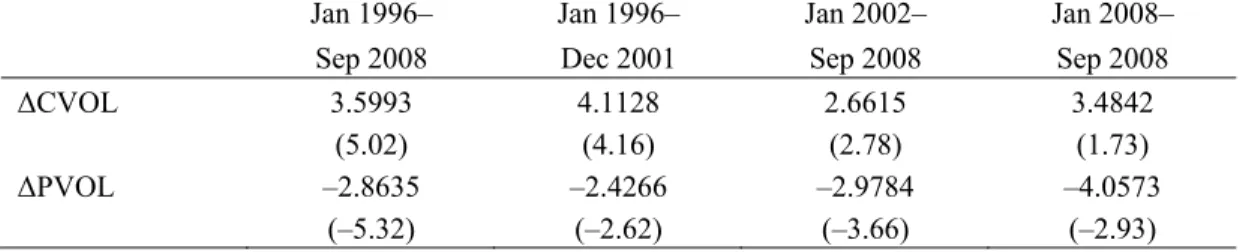
To check whether our results are sensitive to the sample period we report subsample analysis in Table 3 for the bivariate ΔCVOL and ΔPVOL cross-sectional regression. We first decompose the original sample period of January 1996–September 2008 into two subsamples: January 1996 to December 2001 and January 2002 to September 2008. We report the full sample coefficients in the first column, which are identical to regression (10) in Table 2, for comparison. As shown in the second two columns of Table 3, the average slopes on ΔCVOL (ΔPVOL) are positive (negative) and highly significant for both sample periods. The coefficient on ΔCVOL is slightly lower, at 2.66, over the second subsample compared to a value of 3.60 over the whole sample, but is still statistically significant at the 99% level with a Newey-West t-statistic of 2.78. In comparison the coefficients on ΔPVOL are relatively unchanged across the whole sample at –2.86 and across each subsample, with coefficients of –2.43 and –2.98, respectively.
In the last column of Table 3, we investigate the predictive power of ΔCVOL and ΔPVOL during the financial crisis in 2008. During this period volatilities on all stocks increased tremendously. Table 3 reports that the coefficients on both ΔCVOL and ΔPVOL remain positive and negative, respectively, with coefficients of 3.48 and –4.06, respectively. These are similar to the full sample estimates of 3.60 for
ΔCVOL and –2.86 for ΔPVOL. Despite the very short sample of only nine months, the coefficient on
ΔPVOL is even statistically significant with a Newey-West t-statistic of –2.93. Clearly the recent financial crisis has not dented the predictive ability of these variables.
Overall, these results indicate strong significance of the call and put implied volatility shocks as joint determinants of the cross-section of future returns. Increases in call volatilities forecast increases in stock expected returns and increases in put volatilities act in the opposite direction, forecasting decreases in future stock returns.
3.2. Volatility Innovations and Other Cross-Sectional Predictors
Table 4 presents firm-level cross-sectional regressions with volatility innovations measured by first differences from two maturities and other control variables. The first regression in Table 4 reports the coefficients on ΔCVOL and ΔPVOL in the same bivariate cross-sectional regression specification reported in regression (10) from Table 2 for comparison which uses an expiration of 30 calendar days. We also repeat the analysis for option volatilities for an expiration of 91 days in columns (4)-(6).
Regression (2) introduces other risk loadings and characteristics. In the presence of these variables the coefficient on ΔCVOL falls from 3.60 in the bivariate specification (1) to 1.58 in regression (2) but is still significant with a t-statistic of 3.27. The coefficient on ΔPVOL remains almost unchanged at –2.84 with a t-statistic of –4.46 compared to –2.86 in the first column. Thus, the positive coefficient on
12
ΔCVOL and the negative coefficient on ΔPVOL are robust to the standard cross-sectional predictors and have very strong statistical predictability in the presence of the standard risk variables.
In Table 4 the signs of the estimated Fama-MacBeth coefficients on the factors are consistent with earlier studies, but the relations are generally not statistically significant. The log market capitalization (SIZE) and log book-to-market ratio (BM) coefficients indicate a small-large and a value-growth effect with negative and positive coefficients, respectively, but both are insignificantly different from zero. The momentum (MOM) and short-term reversal (REV) effects are also statistically weak. This is because we use optionable stocks that are generally large and liquid where the book-to-market effect is weaker (see Loughran, 1997) . Optionable stocks are significantly different from the usual CRSP universe which contains many more small, illiquid, and low-priced stocks with strong reversal and momentum effects (cf. Hong, Lim and Stein, 2000).
In regression (2) the coefficient on historical volatility, RVOL, is –1.14 and highly statistically significant with a t-statistic of –3.11. This is similar to the cross-sectional volatility effect of Ang et al. (2006, 2009) where stocks with high past volatility have low returns, except Ang et al. work mainly with idiosyncratic volatility defined relative to the Fama and French (1993) model instead of total volatility. Panel B of Table 1 reports that RVOL has very low correlations of 0.04 and 0.05 with ΔCVOL and
ΔPVOL, respectively. This indicates that the effect of past volatility is very different from our cross-sectional predictability of ΔCVOL and ΔPVOL.
We use four additional cross-sectional variables from options in addition to ΔCVOL and ΔPVOL, which are the log call-put ratio of option trading volume (C/P Volume), the log ratio of call-put open interest (C/P OI), the realized-implied volatility spread (RV-IV), and the risk-neutral measure of skewness (QSKEW). The relation between option volume and underlying stock returns has been extensively studied in the literature by Stefan and Whaley (1990), Amin and Lee (1997), Easley, O’Hara, and Srinivas (1998), Chan, Chung, and Fong (2002), Cao, Chen, and Griffin (2005), and Pan and Poteshman (2006), and others.
Pan and Poteshman (2006) find that stocks with high C/P Volume outperform stocks with low call-put volume ratios by more than 40 basis points on the next day and more than 1% over the next week. Our results in Table 5 show that there is a small positive relation, less than 0.03, between C/P Volume and the cross-section of expected returns, but C/P Volume is not significant in regressions (2) and (3). This is consistent with Pan and Poteshman who show that publicly available option volume information contains little predictive power whereas their proprietary measure of option volume from private information does predict future stock returns. As an alternative to option trading volume, we also examine C/P OI. This variable is highly insignificant with a coefficient close to zero.
Bali and Hovakimian (2009) find that stocks with low RV-IV spreads outperform stocks with high RV-IV spread by 63 to 73 basis points in the next month. In regression (3) we include RV-IV but drop the RVOL measure to avoid collinearity. The results in regression (3) confirm the same direction of a relation between a negative RV-IV spread and positive expected returns, but the relation is insignificant at the 95% level. In the presence of RV-IV, the coefficient on ΔCVOL decreases slightly to 1.26 compared to 3.60 in regression (1) and 1.58 in regression (2), but it is still significant at the 95% level. In all three regressions (1)-(3), the coefficient on ΔPVOL remains remarkably unchanged close to –2.9 with t-statistics well below –4.
The last variable in Table 4 is the measure of skewness from option prices, QSKEW. Xing, Zhang and Zhao (2009) find that stocks which exhibit a pronounced degree of negative skewness in option markets, measured by high out-of-the-money put implied volatility compared to at-the-money call implied volatilities, have low returns. On the other hand, Conrad, Dittmar and Ghysels (2009) find the opposite relation with a more general measure of option skewness derived from using the entire cross section of options based on Bakshi, Kapadia and Madan (2003). In regression (2), the coefficient on QSKEW is –3.40 and this carries a highly significant t-statistic of –5.16. This confirms the negative predictive relation between option skew and future stock returns in Xing, Zhang and Zhao (2009). The highly statistically significant loadings on ΔCVOL and ΔPVOL in the presence of the negative QSKEW coefficient imply that the information in option volatility innovations is different from the previously documented predictive ability of the option skew for the cross section of stock returns.
The second set of columns (4)-(6) in Table 4 repeat the same exercise with the Volatility Surface data using a maturity of 91 days. For this maturity we find that the coefficients in the cross-sectional regression controlling for all risk variables on ΔCVOL and ΔPVOL are larger in magnitude and have higher statistical significance than the 30-day maturity coefficients. With the 91-day maturity the
ΔCVOL and ΔPVOL coefficients in regression (5) are 4.37 and –4.73, with t-statistics of 5.70 and –5.79, respectively, compared to 1.58 and –2.85 with t-statistics of 3.27 and –4.46 for the 30-day maturity in regression (2). Volumes for options with longer maturities tend to be lower as these contracts tend to be more illiquid than the shortest maturity option contracts so these results should be interpreted with caution. On the other hand, the Volatility Surface data uses all available option information across all strikes and maturities in the interpolation of the 91-day maturity. Table 4 shows that the longer horizon allows for stronger predictability of the cross section of stocks, perhaps because longer-dated options are more sensitive to directional information captured by ΔCVOL and ΔPVOL on the underlying stocks.
14 The clear conclusion in Table 4 is that cross-sectional regressions with and without risk factors and characteristics provide strong evidence for a significantly positive (negative) relation between the changes in call (put) options’ implied volatilities and future stock returns.
3.3. Time-Series and Cross-Sectional Innovations of Implied Volatilities
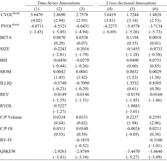
In Table 5 we extend our analysis to the time-series and cross-sectional measures of option volatility innovations. The results in Table 5 echo the main conclusions in Table 4. This is perhaps not surprising since Table 1 shows the correlations between the time-series innovations, shock
ts
CVOL and shock ts
PVOL , and the cross-sectional innovations, shock
cs
CVOL and shock cs
PVOL , with the simple first-difference counterparts
ΔCVOL and ΔPVOL are very high.
First, the average slope coefficients on the CVOL innovation measures are significantly positive. In the cross-sectional regression (2) with risk controls, the coefficient on shock
ts
CVOL is 2.87 with a t-statistic of 2.94. Similarly, the coefficient on the cross-sectional innovation, shock
cs
CVOL , is 1.72 with at t-statistic of 3.14 controlling for other predictors in regression (5).3 In regressions (3) and (6) with RV-IV instead of RVOL, the coefficients on CVOLshockts and CVOLshockcs are similar. Second, put volatility innovations again enter with a highly statistically significant negative sign. These coefficients are larger in absolute value than the coefficients on the call volatility innovations. The implied put volatility time-series (cross-sectional) innovation coefficient in the regression is –4.53 (–3.46), with a t-statistic of –5.05 (–5.26). Again these coefficients are very similar when RV-IV is included as a control variable in regressions (3) and (6). Third, the predictive ability of the call and put innovations estimated from time-series and cross-sectional relations is robust to controlling for the standard predictive characteristics such as SIZE, BM, MOM, and the option predictive variables C/P Volume, C/P OI, RVOL or RV-IV, and QSKEW.
Overall, our findings from the monthly changes and monthly time-series and cross-sectional innovations indicate that unexpected news or information shocks to call and put implied volatilities are able to predict the cross-sectional variation in stock returns.
3 In unreported results we comment that predictive coefficients are slightly larger in absolute value on the
cross-sectional shocks when we augment the regression in equation (4) with one-month lagged realized volatilities for each firm i at time t.
3.4. Systematic vs. Idiosyncratic Volatility Innovations
Implied call and put volatilities contain both systematic and idiosyncratic components. In this section, we investigate if the predictive information in implied volatility innovations reflects news arrivals in systematic risk, idiosyncratic components, or both. This exercise sheds light on whether the forecasting power of call and put volatility innovations is coming from news in risk premium components, at least measured by exposure to the market factor, or by non-market related volatility changes.
We decompose the total implied variance into a systematic component and an idiosyncratic component using a conditional CAPM relation:
2 2 2 2 , , , , , i t i t m t εi t
σ
=β σ
+σ
, (6) where 2 ,t iσ is the risk-neutral variance of stock i, 2 ,t m
σ is the risk-neutral variance of the market m,βi,t is
the market beta of stock i, and
σ
ε2, ,i t is the idiosyncratic risk-neutral variance of stock i, all at time t. We follow Duan and Wei (2009) and estimate the beta from the risk-neutral, not the real, measure to obtain estimates of the systematic and idiosyncratic components of implied volatilities using only option data. This is done by inferring the stock beta from the risk-neutral skewness of the individual stock, Skewi,t, and the risk-neutral skewness of the market, Skewm,t :3/2
, , ,
i t i t m t
Skew =
β
Skew , (7) where the risk-neutral measures of skewness are estimated following Bakshi, Kapadia, and Madan (2003). We provide further details in the Appendix.4We define the systematic and idiosyncratic call implied volatilities as:
,
, , , , , , , , , t m t i t i t i idio t i t m t i sys t iCVOL
CVOL
σ
β
σ
σ
σ
β
ε=
−
=
=
(8) where the betas are estimated from call and put implied volatilities. We use the corresponding expressionssys t i
PVOL, and PVOLidioi,t when put implied volatilities along with the corresponding betas are used to decompose the changes in put implied volatilities. The systematic vs. idiosyncratic decomposition is in terms of standard deviations and follows Ben-Horian and Levy (1980) and others, and it is consistent with our previous empirical work looking at changes in option volatilities, rather than variances. We consider the predictive ability of first-difference innovations
Δ
CVOL
sys,Δ
PVOL
sys,Δ
CVOL
idio, and
4 Christoffersen, Jacobs and Vainberg (2008) argue that betas computed from option prices contain different
16 idio
Δ
PVOL
on the cross section of stock returns. As expected, the cross-sectional correlation of the innovations in the systematic component of volatilities,Δ
CVOL
sysandΔ
PVOL
sys, is very high at above 0.99, whereas the correlation between the idiosyncratic terms,Δ
CVOL
idio andΔ
PVOL
idio, is much lower at 0.64.We report the systematic vs. idiosyncratic decomposition in Table 6. Since the correlation between
Δ
CVOL
sysandΔ
PVOL
sys is close to one, we do not use them simultaneously in one regression to avoid severe multicollinearity. In regressions (1) and (2), the coefficients onΔ
CVOL
sys andsys
Δ
PVOL
are statistically insignificant, whereas the coefficient onΔ
CVOL
idio is positive, reminiscent of the positive coefficient on ΔCVOL in Tables 2-4. The coefficient onΔ
PVOL
idio is negative, also similar to the negative coefficient on ΔPVOL in the previous cross-sectional regressions, showing that only the idiosyncratic components are relatively large in magnitude and carry highly significant t-statistics: in regression (1), the coefficient onΔ
CVOL
idio is 3.18 with a t-statistic of 4.10 and the coefficient onΔ
PVOL
idio is –2.43 with a t-statistic of –4.42. In regression (2), the coefficients onidio
Δ
CVOL
andΔ
PVOL
idio are almost unchanged with effectively the same degrees of significance. Clearly it is changes in the idiosyncratic volatility components that are driving the predictability.Regressions (3)-(6) introduce the same control variables as Tables 2-5 and the finding of that the predictive component in the innovations of call and put volatility changes is idiosyncratic, not systematic, is robust. When the other risk variables and characteristics are introduced, there is a decrease in the coefficient on
Δ
CVOL
idio from 3.2 to around 1.4 and also a smaller decrease in absolute value in the coefficient onΔ
PVOL
idio from –2.4 to around –2.2. However, in all regressions (3)-(6), the coefficients onΔ
CVOL
idio andΔ
PVOL
idio remain significant at the 99% level.In summary, the predictive ability of innovations in call and put volatilities for the cross section of stock returns stems from idiosyncratic, not systematic, components in volatilities. This implies that it is unlikely that the predictability can be explained by systematic risk premiums, at least from market-level returns and aggregate volatility.
4. Returns on Volatility Innovation Portfolios
So far we have documented the predictive ability of option volatility innovations for future stock returns by estimating cross-sectional regressions. In this section we examine the potential investable returns that can be generated by forming portfolios sorted on option implied volatility innovations. In constructing portfolios we are necessarily restricted to using optionable stocks. We concentrate on the simplest measures of option volatility innovations, ΔCVOL and ΔPVOL.
4.1. Portfolios Ranked on ΔCVOL
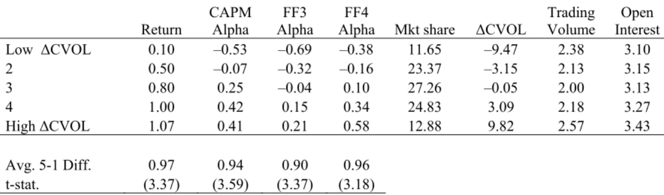
In Panel A of Table 7 we form quintile portfolios ranked on ΔCVOL rebalanced every month. Portfolio 1 (LowΔCVOL) contains stocks with the lowest changes in call implied volatilities in the previous month and Portfolio 5 (High ΔCVOL) includes stocks with the highest changes in call implied volatilities in the previous month. We equal weight stocks in each quintile portfolio. The first panel in Table 7 presents the average raw returns and risk-adjusted returns of the quintile portfolio returns over the whole sample from January 1996 to September 2008. The CAPM alpha is produced by taking the intercept term in a regression of the excess portfolio return on the excess value-weighted market portfolio constructed using all stocks listed on the NYSE, AMEX, and NASDAQ. We denote the alpha produced controlling for the Fama and French (1993) factors by “FF3”. In “FF4” we follow Carhart (1997) and augment the FF3 model by a momentum factor constructed by Kenneth French. Table 7 also reports the average market share, monthly change in call implied volatility (ΔCVOL), monthly trading volume, and open interest of call options in each quintile portfolio. By construction the average monthly ΔCVOL increases across the portfolios from –9.47% for quintile 1 to 9.82% for quintile 5. All the t-statistics reported in Table 7 are computed with robust Newey-West (1987) standard errors.
Panel A shows the average raw return of stocks in quintile 1 with the lowest ΔCVOL is 0.10% per month and this monotonically increases to 1.07% per month for stocks in quintile 5. The difference in average raw returns between quintiles 1 and 5 is 0.97% per month with a highly significant t-statistic of 3.37. This translates to a monthly Sharpe ratio of 0.28 and an annualized Sharpe ratio of 0.98 for a strategy with monthly rebalancing going long High ΔCVOL stocks and shorting Low ΔCVOL stocks. When we perform a CAPM, FF3, and FF4 risk adjustment the differences in alpha between quintile portfolios 1 and 5 are remarkably similar with approximately the same significance levels. In particular, the FF4 alpha difference between the extreme quintiles with the highest and lowest ΔCVOL is 0.96% per month with a t-statistic of 3.18. For the FF4 factor specification, the extreme quintile alphas are
18 themselves significant: the LowΔCVOL FF4 alpha of –0.38% per month has a t-statistic of –2.27 and the FF4 alpha of the High ΔCVOL quintile is 0.58% per month with a t-statistic of 2.21. These results provide strong evidence for an economically and statistically significant, positive relation between
ΔCVOL and expected returns. They complement the positive coefficients on ΔCVOL reported in the cross-sectional regressions of Section 3.
In Panel B of Table 7 we obtain similar results forming quintile portfolios ranked on the percentage change in call implied volatilities, %ΔCVOL. Specifically, the difference in raw average returns between the highest and lowest %ΔCVOL portfolios is 0.92% per month with a t-statistic of 4.07. The average risk-adjusted return differences range from 0.88% to 0.93% per month and are also highly significant. We obtain a similar, strong positive link between the call implied volatility shocks and average returns when forming portfolios using the cross-sectional innovations shock
cs
CVOL as defined in equation (4).
4.2. Portfolios Ranked on ΔCVOL and ΔPVOL
We found in Section 3 that changes in implied put volatilities predicted stock returns but with the opposite sign to call volatilities. We now examine this finding in the context of producing tradable returns by producing double sorts of portfolios ranked on ΔCVOL and ΔPVOL in Table 8. By performing a series of sequential sorts, we produce the portfolio equivalents of placing both ΔCVOL and
ΔPVOL jointly in a bivariate cross-sectional regression.
In Panel A of Table 8 we perform a sequential sort first by creating quintile portfolios ranked by past ΔPVOL. Then, within each ΔPVOL quintile we form a second set of quintile portfolios ranked on
ΔCVOL. This creates a set of portfolios with similar past ΔPVOL characteristics with spreads in ΔCVOL and thus examines expected return differences due to ΔCVOL rankings controlling for the effect of
ΔPVOL. Panel A shows that in each ΔPVOL quintile, the lower (higher) ΔCVOL quintiles have lower (higher) average returns. The column labeled “ΔCVOL5–ΔCVOL1” shows the raw return difference between the High ΔCVOL (ΔCVOL5) and Low ΔCVOL (ΔCVOL1) portfolios within each ΔPVOL quintile. Within the lowest ΔPVOL quintile (ΔPVOL1), the average raw return increases from –0.10% to 1.24% per month when moving from the first to the fifth quintiles. The average raw return difference between ΔCVOL5 and ΔCVOL1 is 1.34% per month with a Newey-West t-statistic of 4.17. This pattern
is repeated across all ΔPVOL quintiles and, with one minor exception, the raw returns are all monotonically increasing as ΔCVOL increases. 5
Panel A also reports the average return difference between highest and lowest quintiles ranked on
ΔCVOL averaged across the ΔPVOL quintiles. This average return difference is 1.13% per month with a t-statistic of 5.39. While the order of magnitude is similar to the raw return difference across extreme quintile portfolios of 0.97% per month in Panel A, Table 7, the statistical significance has increased in Table 8 when we control for the information in ΔPVOL. The difference in FF3 alphas between extreme quintile portfolios ranked on ΔCVOL after controlling for ΔPVOL is very similar at 1.12% per month with a robust t-statistic of 4.95.
In Panel B we repeat the same exercise as Panel A but perform sequential sorts first on ΔCVOL and then on ΔPVOL. This produces sets of portfolios with different ΔPVOL rankings after controlling for the information contained in ΔCVOL. This set of sequential sorts produces lower returns as ΔPVOL increases consistent with the negative coefficients on ΔPVOL in the cross-sectional regressions. For example, in the first ΔCVOL1 quintile, the average raw returns to the quintile with the highest (lowest) past ΔPVOL is 0.27% per month (–0.31% per month). The difference between these extreme quintile returns is –0.58% per month, which is statistically significant at the 95% level. The negative relation between increasing ΔPVOL and lower average returns is repeated in every ΔCVOL quintile and is impressively monotonically decreasing in all cases.
Interestingly, the difference in average returns between the last and first ΔPVOL quintiles is largest for stocks which have experienced the largest changes in CVOL. This is seen in the large –1.44% per month return difference between the extreme ΔPVOL quintiles in the fifth ΔCVOL portfolio. No such skewed pattern is observed in Panel A, which examines the differences in average returns for
ΔCVOL after controlling for ΔPVOL. This indicates that since volatility generally increases for both calls and puts (Table 1 shows the correlation between ΔCVOL and ΔPVOL is 0.57), there are large incremental returns generated by shorting stocks with the largest increases in call volatility and with large put volatility changes.
The last two rows of Table 8, Panel B average the differences between the first and fifth ΔPVOL quintiles across the ΔCVOL quintiles. This summarizes the returns to ΔPVOL after controlling for
ΔCVOL. The average return difference is –0.63% per month with a t-statistic of –4.81. The difference in FF3 alphas is very similar at –0.68% per month with a t-statistic of –5.51. Again there is a strong negative relation between ΔPVOL and stock returns in the cross section.
20
5. Predicting the Cross Section of Implied Volatilities with Stock Returns
Sections 3 and 4 present strong evidence that the cross section of implied volatilities contains valuable information to predict the cross section of stock returns. In this section we examine the other direction of predictability and test if stock returns contain predictive information for the cross section of implied and realized volatilities. We follow our earlier research design and examine one of the very simplest of variables, the change in the stock return, as a proxy for information changes in stock prices, which is analogous to the change in the implied volatility for options.Our empirical tests differ significantly from many studies in the literature investigating the predictability of option volatilities. Many extent studies focus on time-series relations, particularly between implied and realized volatility at the aggregate index level (see, for example, Christensen and Prabhala, 1998, and more recently Chernov, 2007). Bollen and Whaley (2004) examine time-series predictability of 20 individual options focusing on net buying pressure. Dennis and Mayhew (2002) examine cross-sectional predictability of the risk-neutral skewness but do not examine the cross section of implied volatilities. Goyal and Saretto (2009) document that the difference between realized and implied volatilities predicts the cross section of option returns. Naturally, our focus on the cross section of implied volatilities does translate into option holding period returns and we use the realized-implied volatility spread as a control variable, but our variable of interest is much more simple. We study if unusually large returns in underlying equities predict the cross section of implied volatilities.
We examine the significance of information spillover from individual stocks to individual equity options based on the firm-level cross-sectional regressions:
, 1 0, 1, , , 1
, 1 , 1 0, 1, , , 1,
i t t t i t i t
i t i t t t i t i t
CVOL Alpha Controls
CVOL PVOL Alpha Controls
λ
λ
ε
λ
λ
ε
+ + + + + Δ = + ⋅ + + Δ − Δ = + ⋅ + + (9)where the dependent variables, ΔCVOL and ΔPVOL, denote the monthly changes in call and put implied volatilities for stock i over month t to t+1. Alpha is the abnormal return (or alpha) for stock i over the previous month t obtained from the CAPM and the three-factor Fama-French (FF3) model using specifications similar to regression (1). The monthly alphas are computed by summing the daily idiosyncratic returns over the previous month. To test the significance of information flow from stock to options market, the cross-section of implied volatility changes over month t+1 are regressed on the abnormal returns of individual stocks in month t.
The first specification in equation (9) examines how call volatilities over the next month respond to stock returns over the previous month in the Alpha term. The second cross-sectional regression in
equation (9) looks at how call volatilities move relative to put volatilities. Call and put volatility changes, while containing significantly different information for the cross section of equity returns, are correlated at 0.57 (see Table 1). Thus, call and put volatilities tend to move in unison for the same firm. Predicting the spread between put and call implied volatilities, ΔPVOL – ΔCVOL, attempts to control for the common component in both call and put volatilities.
We deliberately do not use option returns as the dependent variable in equation (9). Option returns exhibit marked skewness and have pronounced non-linearities from dynamic leverage making statistical inference difficult (see, among others, Broadie, Chernov and Johannes, 2008; Chaudhri and Schroder, 2009). By focusing on implied volatilities we avoid many of these inference issues.
The control variables we use include market beta, size, book-to-market, momentum, illiquidity, realized volatility, and call and put option trading volume measures.6 Following Bollen and Whaley (2004) and Ni, Pan and Poteshman (2008), we construct ΔOIC and ΔOIP which are the changes in the call and put trading open interest over the previous month, respectively. We also include the RV-IV measure and the risk-neutral measure of skewness, QSKEW.
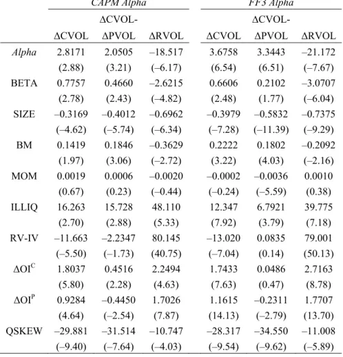
Table 9 presents the average slope coefficients and their Newey-West t-statistics in parentheses. Table 9 reports that for both the CAPM and FF3 alphas, the average slopes on Alpha are positive and
significantly predict both the call and put options’ implied volatility changes over the next month. We find that options where the underlying stocks experienced high abnormal returns over the past month tend to increase their implied volatilities over the next month. Specifically, a 1% CAPM (FF3) alpha over the previous month increases call volatilities by 2.82% (3.68%), on average, with a highly significant t-statistic of 2.88 (6.54). This shows a short-term momentum effect across asset markets with one-month stock momentum positively predicting increases in call implied volatilities.
The positive persistence of lagged stock returns affecting next-period option volatilities is the opposite finding in the literature of the so-called leverage effect, where volatility increases after past low returns (see originally Black, 1976). The leverage effect is a time-series phenomenon where negative shocks to returns contemporaneously increase current volatility and since volatility is persistent, future volatility, on the same stock. The predictive relation in Table 9 is in the cross section where short-term persistence in the stock market filters through to option markets so that call option prices on stocks with high past returns increase next period relative to call options on stocks with low past returns.
6 We do not include short-term reversal (REV) as an additional control variable because of the strong correlation
between REV and the monthly alphas, which leads to a severe multicollinearity problem in cross-sectional regressions. The average correlations among CAPM Alpha, FF3 Alpha, and REV are in the range of 0.92 to 0.96. Hence, predicting the changes in options’ implied volatilities with REV and Alphas produces very similar results.
22 Several of the coefficients on the control variables in Table 9 are interesting results in their own right. As expected from the one-factor decomposition in equation (6), betas are positively related to future volatility changes in the cross section. This goes beyond the finding of Duan and Wei (2009) who show that option levels, not changes, are positively related to the proportion of systematic risk. Increases in volatility are also larger for small firms and value stocks. Underlying stock momentum, MOM, plays no role in determining the cross section of volatility changes. Consistent with Goyal and Saretto (2009), options with large RV-IV tend to predict decreases in implied volatilities and so holding period returns on these options tend to be low. Increases in call and put open interest strongly predict future increases in call and put volatilities. Finally, changes in call (put) implied volatilities tend to be lower (higher) for options where the smile exhibits more pronounced negative skewness.
Table 9 also reports results for cross-sectionally predicting the spread in put and call volatility changes. A stock with a CAPM (FF3) alpha of 1% over the past month has, on average, changes in call volatility 2.05% (3.34%) higher than changes in put volatility. Put another way, momentum in stock returns over the previous month feeds into cross-sectional predictability in option markets. Positive short-term stock momentum tends to produce higher increases in call volatilities relative to put volatilities. It should be noted that from the implied coefficients on predicting ΔPVOL in Table 9, which are positive but much smaller than the coefficients on ΔCVOL, that the implied volatilities of both calls and puts tend to increase when the underlying stock has appreciated. What Table 9 also documents is that call volatilities increase significantly more than put volatilities.
We also test whether the abnormal returns of individual stocks (CAPM, FF3 alphas) can predict the cross-section of realized volatility changes:
Δ
RVOL
i,t+1=
λ
0,t+
λ
1,t⋅
Alpha
i,t+
Controls
+
ε
i,t+1,
(10) where ΔRVOL is the change in realized return volatility of stock i using daily returns from month t to t+1.Table 9 shows that, after controlling for the stock and option characteristics, the cross-sectional regression of ΔRVOL on the CAPM alpha yields an average slope coefficient of –18.52 with a t-statistic of –6.17. Similar results are obtained when the CAPM alpha is replaced by the FF3 alpha; the average slope remains negative at –21.17 with a highly significant with a t-statistic of –7.67. These coefficients are approximately ten times larger in absolute value than in the regressions predicting ΔCVOL and
ΔCVOL – ΔPVOL. The different sign on lagged Alpha to predict next-month ΔRVOL compared to
ΔCVOL is surprising: high past stock returns predict increases in future implied volatilities that are not accompanied by increases in realized volatilities. In fact, future realized volatility tends to decline.
In summary, Table 9 presents strong evidence of cross-asset class predictability at the monthly frequency from stocks to options. On the one hand, positive previous month stock momentum produces increases in call volatilities and higher call versus put volatilities. On the other hand, positive previous one-month stock momentum produces decreases in realized volatilities.
6. Economic Interpretation
The summary of our results is that the cross section of options predicts the cross section of stock returns and vice versa. Both directions of this predictability involve simple changes in prices: changes in option implied volatilities or changes in stock prices over the previous month. Stocks which have experienced large positive changes in call option implied volatility tend to exhibit high expected returns over the next month and stocks with large positive shocks to put option implied volatilities tend to decline over the next month. The returns on portfolios formed by sorting optionable stocks ranked by past changes in call volatility exhibit a spread in average returns and alphas of approximately 1% per month. In the other direction, stocks with abnormal returns of 1% relative to their CAPM beta tend to see call implied volatilities increase over the next month by approximately 3%.
Our findings immediately rule out (noisy) rational expectations models of underlying and derivatives in incomplete markets such as Back (1993), Cao (1999), Buraschi and Jiltsov (2006), and many others. Despite being non-redundant securities, the prices of options in these models immediately adjust to any asymmetric or heterogeneous information possessed by agents, or the costs and incentives of acquiring such information, and thus these models predict that there is no predictability from option to stock markets or vice versa.7
Our results clearly indicate that options and underlying equities play an important role in price formation of both asset markets. Our empirical findings are partly consistent with the microstructure sequential trade model of Easley, O’Hara and Srinivas (1998) in which uninformed liquidity traders place orders in the equity market, the options market, or both. Option markets are not always venues for information-based traders if informed traders cannot satisfactorily hide their trades, but if at least some
7 Much of this literature focuses on the effects of introducing options into incomplete market economies. Because of asymmetric information, Back (1993) and Biais and Hillion (1994) show that introducing an option can cause underlying stock volatility to become stochastic and significantly increase. Most recently, Cao and Yang (2009) show that when options are introduced when agents have differences of opinion, trading volumes reflect the differences of agents’ opinion but all asset prices are formed as if a representative investor existed whose belief reflects the average beliefs across all investors. These issues are not empirically relevant for our results because we have focused on stock returns for which options already exist.
24 informed investors choose to trade in options before trading in underlying stocks, then option prices will predict future stock price movements. Conversely, if stock markets are more liquid and informed traders can more easily hide their trades in equities, then stock markets may lead option markets. Easley, O’Hara and Srinivas find evidence that option volumes of certain types of trades forecast future stock prices within the next hour using intraday data. Motivated from the Easley, O’Hara and Srinivas model, Cremers and Weinbaum (2009) show that deviations from put-call parity document that option prices can predict stock prices by several days.
One key insight of the first microstructure information-based model of Glosten and Milgrom (1985) is that the trading process reveals underlying information and affects the future path of prices. How fast this price adjustment occurs is a key issue. All microstructure models like Easley, O’Hara and Srinivas (1998) are designed to operate at high frequencies and the market maker’s adjustment to informed trades is exponentially fast in terms of the numbers of subsequent trades and since trades for stocks with options occur rapidly, certainly extremely fast in chronological time. The predictability we uncover of the cross-sectional predictability of equity returns by options and vice versa are at the monthly frequency. This is a greater challenge to the microstructure models which are designed to work at high, usually intra-day, frequencies.
We follow an older literature that debates whether options or stocks lead or lag each other. However, these studies were conducted primarily at the daily frequency. Manaster and Rendleman (1982), Bhattacharya (1987), and Anthony (1988) find that options predict future stock prices. Fleming, Ostdiek and Whaley (1996) document options lead the underlying markets using futures and options on futures. In contrast, Stephan and Whaley (1990) and Chan, Chung and Johnson (1993) find stock markets lead option markets. Chakravarty, Gulen and Mayhew (2004) find that both stocks and option markets contribute to price discovery. They find the contribution of option markets to the total variance of common, permanent price movements is around 20%, which is consistent with informed investors trading in both stock and option markets and options playing an important role in price formation. Our findings are very different from this literature because we find that option volatility innovations contain strong predictive power for the cross section of equity returns at the much lower monthly frequency. Similarly, we find a remarkable predictability of past one-month stock returns for future implied volatilities at the monthly frequency.
A more recent literature uses the standard monthly frequency common in the cross-sectional literature to examine how option information predicts underlying stock returns. This literature includes Ofek, Richardson and Whitelaw (2004), Bali and Hovakimian (2009), Cremers and Weinbaum (2009), and Xing, Zhang, and Zhao (2009), who document the predictive ability of various statistics computed
from the cross section of options can predict future equity returns. Our analysis controlled for some of these effects, in particular the option skew examined by Conrad, Dittmar, and Ghysels (2009) and Xing, Zhang and Zhao (2009). None of these papers document that first-difference innovations and other more sophisticated time-series and cross-sectional measures of risk-neutral volatilities predict future returns. This is a surprisingly simple, and strongly significant, measure of news arriving in options markets. Of course, we also find a simple measure of news – past equity returns – forecasts future option volatilities.
Our results on the predictability of equity returns by option information are partly consistent with a more recently developed strand of literature which advocates that investor demand for an option can affect its price. Bollen and Whaley (2004) build a demand-based option model for setting option prices and show that an excess of buyer-motivated traders cause option prices and implied volatility to rise and an excess of seller-motivated trades will cause implied volatility to fa