1-19-2011
A Flexible Spatio-Temporal Model for Air
Pollution: Allowing for Spatio-Temporal
Covariates
Johan Lindstrom
Lund University, johanl@math.lth.se
Adam A. Szpiro
University of Washington, aszpiro@u.washington.edu
Paul D. Sampson
University of Washington - Seattle Campus, pds@stat.washington.edu
Lianne Sheppard
University of Washington, sheppard@u.washington.edu
Assaf Oron
University of Washington, assaf@uw.edu See next page for additional authors
Johan Lindstrom, Adam A. Szpiro, Paul D. Sampson, Lianne Sheppard, Assaf Oron, Mark Richards, and Tim Larson
POLLUTION: ALLOWING FOR SPATIO-TEMPORAL COVARIATES
By Johan Lindstr¨om∗,†, Adam A Szpiro∗, Paul D Sampson∗, Lianne Sheppard∗, Assaf Oron∗, Mark Richards∗, and Tim
Larson∗
University of Washington∗ and Lund University†
AbstractGiven the increasing interest in the association between exposure to air pollution and adverse health outcomes, the develop-ment of models that provide accurate spatio-temporal predictions of air pollution concentrations at small spatial scales is of great impor-tance when assessing potential health effects of air pollution. The methodology presented here has been developed as part of the Multi-Ethnic Study of Atherosclerosis and Air Pollution (MESA Air), a prospective cohort study funded by the US EPA to investigate the relationship between chronic exposure to air pollution and cardiovas-cular disease. We present a spatio-temporal framework that models and predicts ambient air pollution by combining data from several different monitoring networks with the output from deterministic air pollution model(s). The model can accommodate arbitrarily missing observations and allows for a complex spatio-temporal correlation structure.
We apply the model to predict long-term average concentrations of gaseous oxides of nitrogen (NOx) — one of the primary pollutants of
interest in the MESA Air study — during a ten year period in the Los Angeles area, based on measurements from the EPA Air Quality Sys-tem and MESA Air monitoring. The measurements are augmented by a spatio-temporal covariate based on the output from a source dispersion model for traffic related air pollution (Caline3QHC) and the model is evaluated using cross-validation. The predictive ability of the model is good with cross-validated R2
of approximately 0.7 at subject sites.
The incorporation of a dispersion model output into the overall prediction model was feasible, but the particular implementation of Caline3QHC used here did not improve predictions in a model that also includes road information. However, excluding the road infor-mation the inclusion of model output improves predictions and we find some evidence that the source dispersion model can replace road covariates.
The model presented in this paper has been implemented in an R package,SpatioTemporal, which will be available on CRAN shortly.
1. Introduction. There is growing epidemiological evidence of an asso-ciation between exposure to air pollution and adverse health outcomes. The seminal cohort studies were based on assigning exposures using area-wide monitored concentrations in different geographic regions (Dockery et al., 1993; Pope et al., 2002). While straightforward to implement based on reg-ulatory monitoring data, this approach fails to take advantage of variation between individuals living in the same geographic region and may be subject to unmeasured confounding by region.
More recent cohort studies have assigned individual concentrations based on estimates of intra-urban variations in ambient concentrations using nearest-monitor interpolation (Miller et al., 2007; Basu et al., 2000; Ritz et al., 2006; Goss et al., 2004), “land use” regression estimates based on Geographic In-formation System (GIS) covariates (Hoek et al., 2008; Brauer et al., 2003; Jerrett et al., 2005a), geostatistical methods such as kriging (Jerrett et al., 2005b; Kunzli et al., 2005), and semi-parametric smoothing in space and/or time (Kunzli et al., 2005; Puett et al., 2009).
The primary objective of the work described in this paper is develop methods that can be used to produce accurate spatio-temporal predictions of ambient air pollution concentrations for subjects in the Multi-Ethnic Study of Atherosclerosis and Air Pollution (MESA Air). The primary pollutants of interest for MESA Air are particulate matter with aerodynamic diameter less than 2.5 µm (PM2.5) and gaseous oxides of nitrogen (NOx).
MESA Air is a cohort study funded by the Environmental Protection Agency (EPA) with the aim of assessing the relationship between chronic exposure to air pollution and the progression of sub-clinical cardiovascular disease. The MESA Air cohort is comprised of more than 6000 male and female subjects, from six major US metropolitan areas (Los Angeles, CA; New York, NY; Chicago, IL; Minneapolis-St. Paul, MN; Winston-Salem, NC; and Baltimore, MD). The subjects cover four racial/ethnic groups (White, African-American, Hispanic, and Asian, predominantly of Chinese descent) and were aged 45-84 years and free of cardiovascular disease at baseline (see Bild et al., 2002, for details).
A primary focus of the MESA Air study is the development of accurate predictions of ambient air pollution at the home locations of study partici-pants. Combining these predictions with subject-level data — e.g. building infiltration factors, time-activity patterns, and address history — will al-low for subject-specific estimates of chronic ambient source exposure. Using subject-specific exposures, instead of simpler exposure estimates such as the regional average or nearest monitor, provides greater heterogeneity in the exposure estimates. The greater heterogeneity will improve health effect
studies by 1) allowing us to control for confounding between region where appropriate; 2) reducing measurement error from using predicted exposures (Szpiro et al., 2010b; Gryparis et al., 2009; Carroll et al., 2006); and 3) increasing study power.
The primary interest for MESA Air is predicting the chronic exposure of our subjects, but due to several considerations our statistical model needs to account for complex spatio-temporal variability in the data (see Section 3 for details). Overviews of statistical modeling approaches for spatially and spatio-temporally correlated data can be found in Cressie (1993) and Baner-jee et al. (2004). For modeling of spatio-temporally correlated air pollution data, Fanshawe et al. (2008) used carefully selected covariates to eliminate the need for correlated residuals. Several different techniques that allow for complex spatio-temporal dependence structures have been proposed. Two examples are Sahu et al. (2006) and Paciorek et al. (2009), both modeling PM; however these approaches require relatively complete observation ma-trices. Their methods are also developed for much larger geographic regions than those of interest for MESA Air. Smith et al. (2003) handles arbitrary missing observations through an expectation-maximization (EM) algorithm, but their model does not allow for complex spatio-temporal dependencies.
An alternative to statistical modeling is to use numerical models to pro-vide deterministic spatio-temporal predictions of air pollution (Irwin, 2002; Appel et al., 2008). However, when compared to measurements, air quality model output often shows varied prediction performance (Lindstr¨om et al., 2010; Appel et al., 2008; Hogrefe et al., 2006; Mathur et al., 2008). Integrat-ing model output with observations in an attempt to obtain better predic-tions is an active field of research. Most existing studies use output from grid-based models over large geographic areas (e.g., Fuentes and Raftery, 2005; Berrocal et al., 2010; McMillan et al., 2010). Since the MESA Air mod-eling domains are geographically compact we have opted here to combine our observations with the output from a point prediction model (Caline3QHC, described in EPA, 1992b).
Our goal is to construct a general statistical framework that allows us to combine the EPA regulatory and MESA Air supplemental monitoring data (Cohen et al., 2009) with the output of deterministic air pollution mod-els (EPA, 1992b). A spatio-temporal modeling framework for MESA Air has been introduced previously in Sampson et al. (2009) and Szpiro et al. (2010a). Sampson et al. (2009) predicts PM2.5 at subject homes, using a
pragmatic approach that estimates different components of the model sepa-rately and then combines these components to produce predictions. Szpiro et al. (2010a) presents a unified maximum-likelihood estimation method and
studies the statistical properties of the model as well as the added value of MESA Air supplemental monitoring using a simulation study based on a limited set of NOx observations in Los Angeles.
This paper expands on the work of Szpiro et al. (2010a) by: 1) extend-ing the model to include spatio-temporal covariates in order to incorporate output from the Caline3QHC deterministic prediction model; 2) applying the model to the full MESA Air NOx dataset to generate predictions in
Los Angeles; 3) reducing the computational burden by implementing profile likelihood (and restricted maximum likelihood) in order to decrease the di-mension of the optimization problem and by introducing a simplification of the profile likelihood function that decreases the time required for each it-eration; and 4) implementing a novel cross-validation strategy for long-term average predictions that accounts for the complex MESA Air monitoring design. The model presented in this paper has been implemented in an R package, SpatioTemporal, which will be available on the CRAN website shortly.
The available data are described in Section 2. These include observations from both the EPA Air Quality System (AQS) regulatory network and the MESA Air supplemental monitoring, as well as geographic covariates and output from our deterministic air pollution model. Section 3 describes the spatio-temporal model, discusses techniques for efficient parameter estima-tion, and describes our cross-validation approach. Different options for incor-porating the output from our deterministic air pollution model are described in Section 4. In Section 5 we apply the model to NOxdata from Los Angeles
and use cross-validation to assess the model’s predictive ability. Section 6 discusses these results.
2. Description of Data.
2.1. Air Quality System (AQS). The national AQS network of
regula-tory monitors consists of a modest number of fixed sites that measure am-bient concentrations of several different air pollutants including NOx and
PM2.5. Many AQS sites provide hourly averages for NOx, while monitoring
of PM2.5 is less frequent. For this study we include NOx data from 20 AQS
sites in and around Los Angeles.
Since the supplementary MESA Air monitoring is done at the 2-week timescale, we aggregate the AQS data to 2-week averages. The distribution of the resulting 2-week average NOx concentrations is skewed, so we
log-transform the 2-week averages. Examples of time series from three AQS sites are shown in Figure 1; the three sites are located in Glendora, Lynwood, and
Costa Mesa, as indicated on the map in Figure 2. Note the different seasonal patterns and mean levels in the three time series.
Due to maintenance and equipment failures there is some missing data in the AQS monitoring, resulting in a small amount of variability in the number of AQS measurements that contribute to each 2-week average. Periods with less than nine valid measurements have been excluded. This variability can result in different amounts of measurement error. For simplicity we assume a common variance for the measurement error of all AQS and MESA Air 2-week average concentrations (as in Szpiro et al., 2010a).
2.2. MESA Air. The AQS monitors provide data with excellent
tempo-ral resolution, but only at relatively few locations in each of the six cities in the MESA Air study. As pointed out in Szpiro et al. (2010a), potential problems with basing exposure estimates entirely on data from the AQS network are: 1) the number of locations sampled is limited; 2) the AQS network is designed for regulatory rather than epidemiology purposes and does not resolve small scale spatial variability; and 3) the network has sit-ing restrictions that limit its ability to resolve near-road effects. To address these restrictions the MESA Air supplementary monitoring campaign was designed to provide increased diversity in geographic monitoring locations, with specific importance placed on proximity to traffic. The sampling strat-egy and measurement methodology is described in Cohen et al. (2009). We present a brief overview.
The MESA Air supplementary monitoring of ambient outdoor concentra-tions consists of three sub-campaigns: “fixed sites”, “home outdoor”, and “community snapshot”. The campaigns collect 2-week average concentra-tions in each of the six study areas. The fixed and home outdoor campaigns measure PM2.5 and gaseous co-pollutants including NOx, while the snapshot
campaign only measures NOx and other gaseous co-pollutants. Details for
the three MESA Air sub-campaigns follow.
1) The MESA Air fixed sites consist of a few monitors that provided 2-week averages during the entire MESA Air monitoring period. To allow for comparison of different monitoring protocols, at least one MESA fixed site per metropolitan area was colocated with an existing AQS monitor. 2) The home outdoor campaign was designed to obtain information about the con-centration of pollution at participant homes, and consisted of a rotating set of four monitors that were placed at a subset (roughly 10%) of the partici-pants home locations, collecting at least two 2-week averages at each site. 3) The goal of the community snapshot campaign was to collect a spatially rich dataset that could be used to model small scale spatial variability and
road-way effects; and to provide a convenient dataset to guide spatial covariate selection (Mercer et al., 2010). The community snapshot campaign provides three sets of simultaneous measurements of 2-week average concentrations at many locations, including roadway gradients, during three different sea-sons. The roadway gradients consisted of six monitors placed perpendicular to a major roadway (three on either side), at approximately 50, 100, and 150 meters (see Cohen et al., 2009, for details).
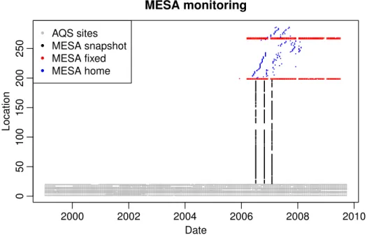
For this paper we restrict attention to sampling in central and costal portion of the Los Angeles basin. A summary of available data, detailing the number of monitor sites, total number of observations, the time periods of the monitoring, and some summary statistics for the observations can be found in Tables 1–2 and Figure 3. Note that one of the MESA fixed sites in the area studied in this paper is colocated with an AQS monitor.
2.3. Geographic Information System (GIS). To predict ambient air
pol-lution at times and locations where we have no measurements we use a complex spatio-temporal model that includes regression with geographic co-variates. Since some of the geographical variables relate to local land uti-lization this approach is often termed “land use” regression (LUR) (Jerrett et al., 2005b). The MESA Air study has created a comprehensive geographic database, and after a preliminary study of the data based on the snapshot campaigns, a subset of the available covariates was selected for use in the present analysis (The selection was based on a preliminary version of the re-sults in Mercer et al., 2010). The covariates used in this paper are: 1) distance to a major road, i.e., census feature class code A1–A3 (distances truncated to be ≥10m and log-transformed), 2) distance to a A1 road (≥10m, log-transformed), 3) total length of A1 and A2 roads in a circular buffer with 300 meter radius, 4) total length of A3 roads in a 50 meter buffer, 5) dis-tance to coast (truncated to be≤15km), and 6) average population density in a 2 km buffer. These are all derived using the ArcGIS (ESRI, Redlands, CA) software package. The distance to coast and roadway variables were ob-tained from Tele Atlas Dynamap 2000 (Lebanon, NH), and the population density was calculated from publicly available Census Bureau data.
2.4. Caline Dispersion Model for Air Pollution. The geographic
covari-ates described above are fixed in time and provide only spatial information. To aid in the spatio-temporal modeling, covariates that vary in both space and time would be valuable. One option is to integrate output from deter-ministic air pollution models into our spatio-temporal model. Several differ-ent air pollution models exist, and in this paper we use a slightly modified version of Caline3QHC (EPA, 1992b; Wilton et al., 2010; MESA Air Data
Team, 2010).
Caline is a line dispersion model for air pollution. Given locations of major sources and local meteorology Caline uses Gaussian dispersion model to pre-dict how nonreactive pollutants travel with the wind away from sources. In contrast to grid-based air pollution models, Caline provides hourly estimates of air pollution at distinct points, called receptors, avoiding the change of support problem inherent in the use of grid based models (e.g. Gotway and Young, 2002; Fuentes and Raftery, 2005).
The Caline predictions we use are based on estimates of traffic density on major roads (A1, A2, and large A3) in the Los Angeles area, obtained from the Southern California Association of Governments. To account for diurnal and weekly variations in traffic patterns, a one week pattern of hourly variations was computed from data provided by the California Department of Transportation. The weekly pattern was repeated for the entire ten-year period and used to modulate the traffic density. The dispersion in Caline is driven by meteorology obtained from the LAX airport meteorology station, and complemented by upper air data from the Radiosonde Database, Earth System Research laboratory, NOAA. We used a unit emissions factor in our Caline implementation.
A final consideration for the Caline computations is the area, or buffer, around each receptor from which pollution is allowed to affect predictions at that receptor. A simplistic interpretation is that the size of the buffer determines how far we believe traffic pollution diffuses during one hour. In preliminary data analysis we studied the effects of several different buffer sizes, ranging from 500 meters to 9 km (the maximum distance recommended by EPA, 1992b). We determined that relatively short buffers are most ap-propriate because the Caline model is most reliable close to nearby sources. In this paper, we use Caline in 500 meter and 3 km buffers. It should be noted that our Caline predictions only include air pollution due to road traf-fic and do not include contributions from point sources. Examples of Caline predictions at three AQS sites are provided in Figure 1.
3. Model and Estimation. The primary interest of the MESA Air study is prediction of long-term averages at subject homes, however several factors necessitate explicit modeling of the 2-week average spatio-temporal field.
First, due to the sampling scheme we only have long-term time series of measurements at a few locations; our other measurements are irregularly distributed in space and time. Since the data exhibit temporal structure that varies with location (see Figure 1), we need to take the full
spatio-temporal structure of the data into account when combining measurements from different locations and times.
Second, modeling 2-week averages allows us to construct long-term av-erages over arbitrary time periods at each location. This makes it possible to calculate exposure based on any hypothesized timescale and to calculate total exposure over the entire study period for participants who have moved within our study area.
We let C(s, t) denote the observed 2-week average concentration of NOx
at location s and time t, where s is a location index taking values in the set {1, . . . , n} and t is in {1, . . . , T}. We let N denote the total number of observations and note that, due to our unbalanced sampling,N ≪nT. Our goal is to predict concentrations at locations and/or times that were not monitored. We denote these unknown values by C∗(s, t). For convenience important notation is summarized in Table 3.
3.1. Hierarchical model. Denoting the logarithm of each two week
aver-age byy(s, t), we decompose the field into
(1) y(s, t) =µ(s, t) +ν(s, t).
Hereµ(s, t) is the predictable mean field andν(s, t) is the essentially random space-time residual field.
We model the mean field as (2) µ(s, t) = L X l=1 γlMl(s, t) + m X i=1 βi(s)fi(t),
where theMl(s, t) are spatio-temporal covariates with coefficientsγl;{fi(t)}mi=1
is a set of smooth basis functions, withf1(t)≡1 andf2(t), . . . , fm(t) having
mean zero; and the βi(s) are spatially varying coefficients for the temporal
trends. See Fuentes et al. (2006) and Szpiro et al. (2010a) for a similar mean field model without spatio-temporal covariates.
In this work we consider a single spatio-temporal covariate, the output from our Caline dispersion model. A possible interpretation of (2) is that we model the mean field as a simple scaling of the contribution from Caline, with a complex additive term that attempts to account for the spatial and temporal variations in air pollution that are not captured by Caline.
The complex additive term, Pmi=1βi(s)fi(t), is a linear combination of
temporal basis functions weighted by coefficients that vary between loca-tions. Typically the number of basis functions will be small. The basis func-tions are derived as smoothed singular vectors using observafunc-tions from the
locations where we have nearly complete time series, i.e. most of the AQS sites; they will be treated as fixed and known for the modeling. Details can be found in Fuentes et al. (2006); Szpiro et al. (2010a); Sampson et al. (2009).
We model the spatial fields ofβi-coefficients using universal kriging (Cressie,
1993). The trend in the kriging is constructed as a linear regression on geo-graphical covariates. The spatial dependence structure is provided by a set of covariance matrices Σβi(θi), which are constructed from a known class of
covariance functions and parameterized by unknown parameter vectors,θi.
The resulting models for theβ-fields are
(3) βi(s)∈N(Xiαi,Σβi(θi)) fori= 1, . . . , m,
where Xi are n × pi design matrices, αi are pi × 1 matrices of regression
coefficients, and Σβi(θi) are n × n covariance matrices. Note that the
de-sign matrices, Xi, can incorporate different geographical covariates for the
different spatial fields. We assume the βi(s) fields are independent of each
other.
Finally, we must specify the model for the residual space-time field,ν(s, t). Following Sampson et al. (2009) and Szpiro et al. (2010a) we assume that the mean model, µ(s, t), accounts for the mean structure and most of the temporal correlation (see Figure 4). We model the residuals as a mean zero Gaussian field that is independent in time and has spatial dependence given by
ν(s, t)∈N0,Σtν(θν)
fort= 1, . . . , T,
where the sizes of the covariance matrices, Σt
ν(θν), are the numbers of
ob-servations, nt, at each time-point. It should be noted that Σtν(θν) does not
imply a time varying covariance matrix; only the number of elements in Σt
ν(θν) vary for different t. Elements in the covariance matrices are defined
by assuming a known class of covariance functions that is parameterized by a set of unknown parameters,θν.
We have assumed that the covariance matrices are constructed by plug-ging unknown parameters (which will have to be estimated) into a known class of covariance functions (e.g., one of those described in Cressie, 1993). It should be noted that there is nothing in the model that requires the dif-ferent spatial fields to share a common covariance structure. This allows any non-stationarity in the space-time residuals to be accommodated using, e.g., deformation methods (Sampson, 2002; Damian et al., 2003), while retaining a stationary covariance structure for theβi-fields.
Here we use exponential covariance functions, characterized by rangeφ, partial sill σ2, and nugget τ2. To obtain a smooth mean field in (2) we assume that the nuggets of the βi-fields are zero. Thus, the parameters of
the model consist of: the regression parameters for the geographical, and spatio-temporal covariates, respectively
α= (α⊤1, . . . , α⊤m)⊤; γ= (γ1, . . . , γL)⊤,
spatial covariance parameters for theβi-fields,
θB= (θ1, . . . , θm) where θi = (φi, σ2i),
and covariance parameters of the spatio-temporal residuals,
θν = (φν, σ2ν, τν2).
To simplify notation we collect the covariance parameters into Ψ, Ψ = (θ1, . . . , θm, θν).
Combining (1) and (2) our model becomes (4) y(s, t) = L X l=1 γlMl(s, t) + m X i=1 βi(s)fi(t) +ν(s, t).
Following Szpiro et al. (2010a), we introduce theN ×1-vectors Y =y(s, t) and V = ν(s, t) by stacking the elements into single vectors varying first
s and then t; a mn × 1-vector B = (β1(s)⊤, . . . , βm(s)⊤)⊤; and a sparse
N × mn-matrix F = (fst,is′) with elements fst,is′ =
(
fi(t) s=s′
0 otherwise.
To accommodate the spatio-temporal covariates we also introduce aN ×L -matrixM, with each row containing covariates for the space-time location of the corresponding row inY.
Using these matrices we rewrite (4) as (5) Y =Mγ+F B+V,
where
Here X, ΣB(θB), and Σν(θν) are block diagonal matrices with diagonal blocks{Xi}mi=1,{Σβi(θi)} m i=1, and Σt ν(θν) T
t=1 respectively. Noting that (5)
is a linear combinations of Gaussians we introduce the matrices
e
X =hM F Xi and Σ(Ψ) = Σe ν(θν) +FΣB(θB)F⊤,
and write the distribution ofY as (6) [Y|Ψ,γ,α]∈N Xe " γ α # ,Σ(Ψ)e ! .
Estimating the unknown parameters, (Ψ,γ,α), can now be accomplished
by maximizing the log-likelihood
2l(Ψ,γ,α|Y) =−Nlog(2π)−log eΣ(Ψ) − Y −Xe " γ α #⊤ e Σ−1(Ψ) Y −Xe " γ α # . (7)
3.2. Parameter estimation. Given the large monitoring database,
esti-mating parameters by na¨ıve maximum likelihood (ML) takes considerable computer time. There are two considerations of importance for minimizing the required computer time: 1) reducing the number of parameters should speed up the estimation, and 2) the block structure of Σν(θν) and ΣB(θB)
can be exploited to reduce the computational burden of evaluating the log-likelihood.
It is trivial to show that the generalized least-squares fit
" γ(Ψ) α(Ψ) # =Xe⊤Σe−1(Ψ)Xe−1Xe⊤Σe−1(Ψ)Y (8)
maximizes the log-likelihood with respect to γ and α, for any values of Ψ.
Replacing γ and α with the functions of Ψ obtained in (8) reduces the
unknown parameters in the log-likelihood to only Ψ. This corresponds to the profile log-likelihood which, after some algebra, is
2lprof(Ψ|Y) =−Nlog(2π)−log
eΣ(Ψ)−Y⊤Σe−1(Ψ)Y
+Y⊤Σe−1(Ψ)XeXe⊤Σe−1(Ψ)Xe−1Xe⊤Σe−1(Ψ)Y.
(9)
Note that the value Ψ that maximizes the profile likelihood also maximizes the original likelihood (7).
The profile likelihood reduces the number of unknown parameters but it does not utilize the block structure of Σν(θν) and ΣB(θB). A way of
rewrit-ing (9) that utilizes the structure to significantly reduce the computational burden is provided in Appendix A. As an example, evaluating the likeli-hoodoncefor our 5181 measurements in Los Angeles takes 92 seconds using the original profile likelihood formulation (9), compared to 2.5 seconds af-ter simplifications (on an Intel Xeon E5410 processor). Figure 5 provides comparisons of evaluation times for different size datasets. Both the faster evaluation time for the optimized likelihood, as well as the much slower increase in computation time as a function of dataset size, both in terms of number of observations and number of spatial locations, are illustrated. Additional theoretical details regarding the computational burden can be found in Appendix A.2.
We use the constrained L-BFGS-B algorithm implemented in theoptim()
function in R (Byrd et al., 1995; R Development Core Team, 2008) to op-timize the profile likelihood, first log-transforming the covariance parame-ters to make the optimization easier. We denote the estimated parameparame-ters by Ψbprof, γbprof, and αbprof. To obtain approximate uncertainties for the
estimated parameters we compute the finite difference Hessian of the full log-likelihood and take the negative diagonal elements of its inverse (i.e., we use the observed information matrix).
3.2.1. Restricted Maximum Likelihood. An alternative option for reduc-ing the number of parameters is restricted maximum likelihood (REML) (Patterson and Thompson, 1971; Harville, 1974). In classical statistical terms, the principal difference between profile likelihood (equivalently ML) and REML is that REML accounts for the loss in the degrees of freedom associ-ated with estimation of the regression parameters,γandα, when estimating
the covariance. A Bayesian interpretation is that REML assumes flat priors and marginalizes the full likelihood with respect to γ and α (see Harville,
1974, for details).
Simulation studies indicate that REML estimates of variance parameters are less biased than ML estimates (Swallow and Monahan, 1984; Cressie and Lahiri, 1993). However, due to the bias-variance trade-off, ML estimates can exhibit smaller mean squared errors than REML estimates for some models (Swallow and Monahan, 1984). Further, the magnitude of the bias in ML depends on the number of regression parameters compared to the number of observations and decreases with increasing sample size. In this study we use the profile likelihood, but for completeness parallel results for REML are given in Appendix B.
The primary reason we prefer profile likelihood is that it is equivalent to ML, and our predictions will be used as exposures in a health effects model where it is natural to account for the joint variability of all the estimated exposure model parameters using the full likelihood (Szpiro et al., 2010b). Also, in a simple simulation study based on parts of our data we found a small bias reduction from using REML, but the numerical estimation for REML was significantly more time consuming and prone to non-convergence.
3.3. Prediction. Having obtained values for the parameters the next step
is to predict concentrations at unobserved locations and times. As previously noted we let C∗(s, t) denote these unobserved values. By adding the unob-served times and locations to our model we expand the distribution in (6) to includey∗(s, t) = logC∗(s, t), or (10) Y Y∗ Ψ,γ,α ∈N " e X e X∗ # " γ α # , " e Σ··(Ψ) Σe·∗(Ψ) e Σ⊤ ·∗(Ψ) Σe∗∗(Ψ) #! ,
whereΣe··is the covariance matrix for the observed data,Σe∗∗is the covariance
for the unobserved data, andΣe·∗ is the cross-covariance between observed
and unobserved data. Finally Xe∗ is constructed using the spatio temporal covariates, temporal trends, and geographical covariates for the unobserved data.
Predictions and prediction uncertainties are obtained as the conditional expectation and conditional variance of (10). The prediction variance is (11) V Y∗Y,Ψbprof,γbprof,αbprof,
=Σe∗∗−Σe·∗⊤Σe−··1Σe·∗
where all the covariance matrices are evaluated atΨbprof.
The approximate parameter uncertainties are computed using the ob-served information matrix and are based on asymptotic maximum likelihood theory (see, e.g. Casella and Berger, 2002); the prediction uncertainties (11) do not account for uncertainties in the estimated parameters. One option for obtaining full prediction uncertainties is to use Markov Chain Monte Carlo (MCMC) (Metropolis et al., 1953; Hastings, 1970) or some other nu-merical integration scheme (Rue et al., 2009). An appealing option when us-ing MCMC is to first maximize the likelihood usus-ing numerical optimization and then use the observed information matrix to construct a Metropolis-random-walk-algorithm with optimal proposal distribution (Gelman et al., 1996). This approach is implemented in our R package, SpatioTemporal. Using MCMC, however, adds considerable computer time and is not feasible for our cross-validation study.
3.4. Validation. We use cross-validation to assess the predictive accuracy of our model. Our primary interest is the prediction of long-term averages, but we have only 25 monitors (AQS and MESA fixed sites) that provide time series against which we can validate predictions of long-term averages. Due to AQS siting, these 25 monitors have less heterogeneity in their geo-graphic covariates but larger spatial spread when compared to participant home locations, potentially limiting our ability to correctly assess model performance.
To make the fullest use of available data we employ three different cross-validation strategies: 1) leave-one-out cross-cross-validation for the AQS and MESA fixed sites (the two colocated sites are kept together, resulting in 24 groups), 2) 10-fold cross-validation for the sites in the snapshot campaign (ensuring not to split road gradients between groups); and 3) 10-fold cross-validation of the home outdoor sites. For each of the scenarios above, all remaining data are used to estimate parameters and to predict at the left out loca-tions. Given the predictions and prediction variances (11) we compute the coverage for 95% prediction intervals, the root mean squared error (RMSE) and the corresponding cross-validated R2.
For the first cross-validation approach we validate the model by compar-ing predicted and observed 2-week averages, as well as the predicted and observed long-term average concentration at each location. To compute the true long-term averages we use time points for which we have observations at that location, and we compute predicted long-term averages using the predicted 2-week average concentrations at the corresponding times,
C∗(s) = X
t∈{τ:∃y(s,τ)}
exp(y∗(s, t))
k{τ : ∃y(s, τ)}k.
The cross-validatedR2 are computed as
R2= max 0,1− RMSE 2 Var(C(s)) .
For the MESA Air snapshot campaign, we calculate cross-validated pre-dictions by simultaneously leaving out measurements in the validation set for all three seasons. However, when assessing the spatial predictive ability of our model, we compute separate RMSE and R2 values for each season. This has the added benefit of providing information regarding the model’s differential spatial predictive ability in each season.
For the MESA Air home campaign the situation is slightly more compli-cated since our measurements are spread out in time and space. We compute
the RMSE value as usual, but forR2 we compare our predictions to a sim-ple reference model that accounts for the temporal variability. We use the formula R2 = max 0,1− RMSE 2 RMSE2ref ,
where RMSE2refdenotes the RMSE of a reference model to which we compare our predictions. Reference models used are: 1) the spatial average at each time point based on observations at AQS and MESA fixed sites; 2) the closest available observation from the AQS and MESA fixed sites; 3) smooth temporal trends fitted to the data at the closest AQS or MESA fixed sites. These three reference models will be denoted asaverage,closest, andsmooth
in the rest of this document. ThisR2 can also be seen as the improvement in prediction provided by our model when compared to the use of the central site or nearest neighbor schemes common in published epidemiology studies (Pope et al., 1995; Goss et al., 2004; Miller et al., 2007).
4. Different ways of including Caline. We have considered several different options for including the Caline predictions in the spatio-temporal model. Because our observations are log-transformed, a similar transfor-mation of Caline seems reasonable. However, since the Caline predictions include contribution from major roads within the 500m or 3km buffers, we use a log(x+ 1) transformation to accommodate zeros. Preliminary studies with no transformation, or including first, second, and third order terms to account for potential non-linearities indicated results similar to, or worse than, the log(x+ 1) transformation.
A second issue is that the unbalanced monitoring scheme, with long-time series at a few sites, may cause the model fit to emphasize Caline’s temporal predictive ability over its spatial features. Therefore, we also consider the performance of a mean separated Caline variable. For the mean separated Caline, we takeM(s, t) = log(Caline + 1), compute the temporal average at each location M(s) = 1 T X t M(s, t),
and calculate a new spatio-temporal covariate that is mean-zero at each site
f
M(s, t) =M(s, t)− M(s).
The average,M(s), is added to the list of geographic covariates andMf(s, t) is used as a spatio-temporal covariate, allowing us to separate Caline’s spa-tial and temporal contributions to the predictions.
5. Results.
5.1. Geographic covariate predictors only (no Caline). Cross-validation
results for the model with only geographic covariates (no Caline) are pre-sented in Table 4. Figure 6 shows the cross-validated predictions, along with observed data and prediction intervals at three AQS sites, and Figure 7 shows predictions of long-term averages at the AQS and MESA fixed sites. The estimated parameters for the model fit to all the data are given in Table 7.
The predictive ability at MESA home sites is very good, withR2 ≈0.9. Even after the use of a simple reference model to account for the temporal variability, the spatial predictive ability remains high, withR2≈0.67−0.74 depending on the reference model used. TheR2 values are slightly lower for the summer snapshot (R2 ≈0.52) and long-term averages (R2 ≈0.58). The lowest RMSE values are also found during the summer snapshot, indicating that there is little variability to explain in this dataset. The lowerR2 values for the long-term averages are also expected because many AQS sites are either far from other sites or at the edge of our area of interest (see the map in Figure 2). Due to the spatial dependence in our model, we expect cross-validation at these sites to exhibit larger prediction errors than at subject home locations. Our uncertainty estimates are also reasonable, with the coverage for 95% prediction intervals varying from 91% to 99% for all three cross-validation approaches.
5.2. Geographic covariates and Caline predictors. Our primary
imple-mentation of Caline is mean separated with a 3 km buffer. Results for the version that is not mean separated and for a 500 meter buffer are similar or slightly worse (see Table 5). The estimated parameters for the model with and without Caline are compared in Table 7. It is worth noting that the estimated coefficient for the contribution from the time averaged Caline to the spatial intercept (the Caline coefficient in β1) is statistically
signifi-cant as is the contribution from the spatio temporally varying Caline (the
γ-coefficient). Several of the regression coefficients for the temporal trends (β2 and β3) are not significant, however attempts to reduce the number of
covariates for theβ2andβ3 fields decreased the cross-validated performance.
Coefficients for the other geographic covariates are very similar in the model with and without Caline. Cross-validation results for the model with Caline are given in Table 4. For this implementation there is no evidence of im-proved performance compared to the model without Caline.
One possible explanation for the lack of improvement from Caline is that the model already contains road covariates that are good predictors of traffic
related NOx. In an attempt to compare the predictive ability of road
covari-ates with that of Caline, we fit the model again without any of the GIS road covariates, with and without Caline. Estimated parameters for both models are presented in Table 8. The estimated parameters for the twoβ-fields that affect the temporal trends are very similar, indicating that the variation in temporal trends over the region is not primarily driven by local road/traffic effects. For the long-term averageβ1-field there are differences in estimated parameters. The effect of population density is almost halved when Caline is included, and the estimated range parameter for β1 is only 530 m
with-out Caline, compared to 3.7 km when including Caline. The coefficient for Caline in theβ1-field is much larger than in the model with road covariates
(0.145 compared to 0.0789), indicating that without the road covariates the contribution from Caline is more important.
Cross-validation results are presented in Table 6 and Figure 7. With-out the road covariates in the model, including Caline results in uniformly better cross-validation results than for the model without Caline. In fact, predictions with this model are nearly comparable to those obtained from the model that includes road covariates but not Caline. This suggests that our implementation of Caline may be able to provide interpretable replace-ment for GIS road covariates, even though it does not provide additional predictive power in a model that already includes roadway information.
6. Discussion. In this paper we have expanded the spatio-temporal framework introduced by (Sampson et al., 2009; Szpiro et al., 2010b) to allow for spatio-temporally varying covariates. The resulting model provides a flexible way of combining observations with the output from deterministic air quality models. The model presented in this paper has been implemented in an R-package, SpatioTemporalthat will be available on CRAN shortly.
To make the model computationally feasible, we used profile likelihood (and REML) to reduce the number of parameters that have to be estimated. Further, the structure in the model, with spatially correlated but temporally independent residuals, allowed us to rewrite the likelihood into a computa-tionally efficient form. The importance of these simplifications cannot be stressed enough, as they reduce the computational burden by more than an order of magnitude.
The model was applied to the full MESA Air dataset in Los Angeles, and a thorough cross-validation study was done to evaluate prediction per-formance. In order for us to make the fullest use of the unbalanced moni-toring in the MESA Air study, special care was taken when designing the cross-validation study in order to focus on predicting long-term averages,
even though much of our validation data are collected over short time pe-riods. The cross-validation study shows good predictive power, especially at subject home locations. This indicates that our spatio-temporal model will be able to provide the basis for high quality predicted exposures in our health analysis. Furthermore, our profile likelihood estimation methodology provides uncertainty estimates suitable for use in our recently developed methods to adjust for measurement error that results from using predicted exposures in place of the true values (Szpiro et al., 2010b).
Including Caline as an additional predictor variable provided essentially no overall improvement in prediction accuracy. This came as somewhat of a surprise to the authors, especially since a previous pilot study (Wilton et al., 2010) indicated improved prediction performance for the summer snapshot. However, consistent with the pilot study, we find some improvement for the summer snapshot when including Caline (see Table 4). One reason for this lack of improvement may be that we used a constant unit emissions fatcor that does not account for changes to the fleet over time. As future research we will weight our Caline predictions by including trends in fleet emissions (by e.g. using the EPA’s MOVES model; EPA, 1992a). Our results do, however, suggest that Caline may provide a more directly interpretable replacement for GIS road covariates, potentially limiting the need for model selection from multiple road covariates corresponding to different road classes and buffer sizes.
Our results contrast with other studies that have shown improvement in air quality predictions by combining observations with output from de-terministic models (e.g. Fuentes and Raftery, 2005; Berrocal et al., 2010; McMillan et al., 2010). These studies do not use any GIS covariates, but do use output from grid based models over large geographic areas, often several states. These differences make it difficult to translate their results to our limited geographic areas and study design. Given the relatively compact geographical areas in the MESA Air study and our need to resolve small-scale spatial variability, the potential gain from grid based models is limited. The most commonly used model, EPA’s Community Multiscale Air Qual-ity (CMAQ), produces predictions on 4, 12, or 36 km grids (most typically 12 km). With a 12 km grid our Los Angeles study area can be covered using only 30 grid cells, so a grid-based model of this resolution would provide limited spatial information over our study area.
Acknowledgments. Although the research described in this article has been funded wholly or in part by the United States Environmental Pro-tection Agency through assistance agreement CR-834077101-0 and grant
RD831697 to the University of Washington, it has not been subjected to the Agency’s required peer and policy review and therefore does not neces-sarily reflect the views of the Agency and no official endorsement should be inferred.
Travel for Johan Lindstr¨om has been paid by STINT (The Swedish Foun-dation for International Cooperation in Research and Higher Education) Grant IG2005-2047.
Additional funding was provided by grants to the University of Wash-ington from the Health Effects Institute (4749-RFA05-1A/06-10) and the National Institute of Environmental Health Sciences (P50 ES015915).
The MESA cohort study is supported by contracts N01-HC-95159 through N01-HC-95169 from the National Heart, Lung, and Blood Institute. The authors thank the other investigators, the staff, and the participants of the MESA study for their valuable contributions. A full list of partici-pating MESA investigators and institutions can be found at http://www. mesa-nhlbi.org.
References.
Appel, K. W., Bhave, P. V., Gilliland, A. B., Sarwar, G. and Roselle, S. J. (2008). Evaluation of the community multiscale air quality (CMAQ) model version 4.5: Sensitivities impacting model performance; part II-particulate matter.Atmo. Environ., 426057–6066.
Banerjee, S.,Carlin, B. P. andGelfand, A. E. (2004). Hierarchical Modeling and Analysis for Spatial Data. Chapman and Hall, CRC.
Basu, R., Woodruff, T. J., Parker, J. D.,Saulnier, L. and Schoendorf, K. C. (2000). Particulate air pollution and mortality: Findings from 20 U.S. cities. N. Engl. J. Med.,3431742–1749.
Berrocal, V. J., Gelfand, A. E. and Holland, D. M. (2010). A spatio-temporal downscaler for output from numerical models. J. Agric. Bio. and Environ. Statist.
Bild, D. E.,Bluemke, D. A.,Burke, G. L.,R., D.,Diez Roux, A. V.,Folsom, A. R., Greenland, P.,Jacob, D. R., Jr,Kronmal, R.,Liu, K.,Nelson, J. C.,O’Leary, D.,Saad, M. F.,Shea, S.,Szklo, M.andTracy, R. P.(2002). Multi-ethnic study of atherosclerosis: Objectives and design.American Journal of Epidemiology,156871– 881.
Brauer, M., Hoek, G.,van Vliet, P.,Meliefste, K.,Fischer, P., Gehring, U., Heinrich, J.,Cyrys, J.,Bellander, T.,Lewne, M.andBrunekreef, B.(2003). Estimating long-term average particulate air pollution concentrations: Application of traffic indicators and geographic information systems. Epidemiology,14228–239. Byrd, R.,Lu, P.,Nocedal, J. andZhu, C.(1995). A limited memory algorithm for
bound constrained optimization. SIAM J. Sci. Comput.1190–1208.
Carroll, R. J., Ruppert, D., Stefanski, L. A. and Crainiceanu, C. M. (2006).
Measurement Error in Nonlinear Models: A Modern Perspective. 2nd ed. Chapman and Hall, CRC.
Casella, G.andBerger, R. L.(2002). Statistical Inference. 2nd ed. Duxbury. Cohen, M. A.,Adar, S. D.,Allen, R. W.,Avol, E.,Curl, C. L.,Gould, T.,Hardie,
K. D.,Swan, S. S.,Liu, L.-J. S.andKaufman, J. D.(2009). Approach to estimating participant pollutant exposures in the Multi-Ethnic Study of Atherosclerosis and air pollution (MESA air). Environ. Sci. Technol.,434687–4693.
Cressie, N.(1993). Statistics for Spatial Data. Revised ed. John Wiley & Sons Ltd. Cressie, N. and Lahiri, S. (1993). The asymptotic distribution of reml estimators.
Journal of Multivariate Analysis,45217–233.
Damian, D.,Sampson, P. D.andGuttorp, P.(2003). Variance modeling for nonsta-tionary processes with temporal replications. J. Geophys. Res.,1088778.
Dockery, D. W.,Pope, C. A.,Xu, X.,Spangler, J. D.,Ware, J. H.,Fay, M. E., Ferris, B. G.andSpeizer, F. E. (1993). An association between air pollution and mortality in six cities. N. Engl. J. Med.,3291753–1759.
EPA(1992a). Technical guidance on the use of MOVES2010 for emission inventory prepa-rationin state implementation plans and transportation conformity. Tech. Rep. EPA-420-B-10-023, U.S. Environmental Protection Agency.
EPA(1992b). User’s guide to CAL3QHC version 2.0: A modeling methodology for predict-ing pollutant concentrations near roadway intersections. Tech. Rep. EPA-454/R-92-006, U.S. Environmental Protection Agency, Research Triangle Park, NC, USA.
Fanshawe, T. R., Diggle, P. J., Rushton, S., Sanderson, R., Lurz, P. W. W., Glinianaia, S. V.,Pearce, M. S.,Parker, L.,Charlton, M.andPless-Mulloli, T. (2008). Modelling spatio-temporal variation in exposure to particulate matter: a two-stage approach. Environmetrics,19549–566.
Fuentes, M.,Guttorp, P.andSampson, P. D.(2006). Using transforms to analyze space-time processes. InStatistical Methods for Spatio-Temporal Systems (B. Finken-stadt, L. Held and V. Isham, eds.). CRC/Chapman and Hall, 77–150.
Fuentes, M.andRaftery, A. E.(2005). Model evaluation and spatial interpolation by Bayesian combination of observations with outputs from numerical models.Biometrics, 6134–45.
Gelman, A.,Roberts, G.andGilks, W.(1996). Efficient metropolis jumping rules. In
Bayesian Statistics 5 (J. M. Bernardo, J. O. Berger, A. P. Dawid and A. F. M. Smith, eds.). Oxford University Press, 599–607.
Goss, C. H.,Newsom, S. A.,Schildcrout, J. S.,Sheppard, L.andKaufman, J. D. (2004). Effect of ambient air pollution on pulmonary exacerbations and lung function in cystic fibrosis. Am. J. Respir. Crit. Care med.,169816–821.
Gotway, C. and Young, L. (2002). Combining incompatible spatial data. J. Amer. Statist. Assoc.,97632–648.
Gryparis, A., Paciorek, C. J., Zeka, A., Schwartz, J. and Coull, B. A. (2009). Measurement error caused by spatial misalignment in environmental epidemiology. Bio-statistics,10258–274.
Harville, D. A.(1974). Bayesian inference for variance components using only error contrasts. Biometrika,61383–385.
Harville, D. A. (1997). Matrix Algebra From a Statistician’s Perspective. 1st ed. Springer.
Hastings, W. (1970). Monte Carlo sampling methods using Markov chains and their applications. Biometrika,5797–109.
Hoek, G., Beelena, R., de Hoogh, K., Vienneaub, D., Gulliverc, J., Fischer, P. and Briggs, D. (2008). A review of land-use regression models to assess spatial variation of outdoor air pollution. Atmo. Environ.,427561–7578.
Hogrefe, C.,Porter, P.,Gego, E.,Gilliland, A.,Gilliam, R.,Swall, J.,Irwin, J.andRao, S.(2006). Temporal features in observed and simulated meteorology and air quality over the eastern united states. Atmo. Environ.,405041–5055.
Irwin, J. S.(2002). A historical look at the development of regulatory air quality models for the United States Environmental Protection Agency, vol. 244 of NOAA technical memorandum OAR ARL. U.S. Dept. of Commerce, National Oceanic and Atmospheric Administration.
Jerrett, M., Arain, A., Kanaroglou, P., Beckerman, B., Potoglou, D., Sah-suvaroglu, T.,Morrison, J. and Giovis, C. (2005a). A review and evaluation of intraurban air pollution exposure models. J. Exposure Anal. Environ. Epidemiol.,15 185–204.
Jerrett, M.,Burnett, R. T.,Ma, R.,Pope, C. A.,Krewski, D.,Newbold, K. B., Thurston, G.,Shi, Y.,Finkelstein, N.,Calle, E. E. andThun, M. J.(2005b). Spatial analysis of air pollution mortality in Los Angeles. Epidemiology,16727–736. Kunzli, N., Jerrett, M., Mack, W. J., Beckerman, B., LaBree, L., Gilliland,
F., Thomas, D.,Peters, J. and Hodis, H. N. (2005). Ambient air pollution and atherosclerosis in Los Angeles. Environ. Health Persp.,113201–206.
Lindstr¨om, J., Sampson, P. D., Guttorp, P. and Sheppard, L. (2010). Spurious correlations; potential pitfalls when evaluating air quality models against observations.
In preparation.
Mathur, R.,Yu, S.,Kang, D.andSchere, K. L.(2008). Assessment of the wintertime performance of developmental particulate matter forecasts with the EPA-Community Multiscale Air Quality modeling system. J. Geophys. Res.,113D02303.
McMillan, N. J., Holland, D. M., Morara, M.and Feng, J. (2010). Combining numerical model output and particulate data using bayesian space-time modeling. En-vironmetrics,2148–65.
Mercer, L.,Szpiro, A. A.,Sheppard, L.,Adar, S.,Allen, R.,Avol, E.,Lindstr¨om, J.,Oron, A.,Larson, T.,Liu, L.-J. S.and Kaufman, J. (2010). Predicting con-centrations of oxides of nitrogen in Los Angeles, CA using universal kriging. TBD,? Work in progress.
MESA Air Data Team (2010). Documentation of MESA air implementation of the Caline3QHCR model. Tech. rep., University of Washington, Seattle, WA, USA. Metropolis, N., Rosenbluth, A., Rosenbluth, M., Teller, A. and Teller, E.
(1953). Equations of state calculations by fast computing machines. J. Chem. Phys., 211087–1092.
Miller, K. A.,Sicovick, D. S.,Sheppard, L.,Shepherd, K.,Sullivan, J. H., An-derson, G. L.andKaufman, J. D.(2007). Long-term exposure to air pollution and incidence of cardiovascular events in women. N. Engl. J. Med.,356447–458.
Paciorek, C. P.,Yanosky, J. D.,Puett, R. C.,Laden, F. andSuh, H. H.(2009). Practical large-scale spatio-temporal moeling of particulate matter concentrations.Ann. Statist.,3370–397.
Patterson, H. D.andThompson, R.(1971). Recovery of inter-block information when block sizes are unequal. Biometrika,58545–554.
Pope, C. A., Burnett, R. T., Thun, M. J., Calle, E. E., Krewski, D., Ito, K. andThurston, G. D.(2002). Lung cancer, cardiopulmonary mortality, and long-term exposure to fine particulate air pollution. J. Am. Med. Assoc.,91132–1141.
Pope, C. A., Thun, M. J., Namboodiri, M. M., Dockery, D. W., Evans, J. S., Speizer, F. E.andHeath, C. W., Jr.(1995). Particulate air pollution as a predictor of mortality in a prospective study of U.S. adults. Am. J. Respir. Crit. Care med.,151 669–674.
Puett, R. C.,Hart, J. E.,Yanosky, J. D.,Paciorek, C. J.,Schwartz, J.,Suh, H., Speizer, F. E.and Laden, F.(2009). Chronic fine and coarse particulate exposure, mortality and coronary heart disease in the nurses’ health study.Environ. Health Persp.,
1171697–1701.
R Development Core Team(2008). R: A Language and Environment for Statistical Computing. R Foundation for Statistical Computing, Vienna, Austria. ISBN 3-900051-07-0, URLhttp://www.R-project.org.
Ritz, B.,Wilhelm, M.andZhao, Y.(2006). Air pollution and infant death in southern California, 1989-2000. Pediatrics,118493–502.
Rue, H., Martino, S. and Chopin, N. (2009). Approximate Bayesian inference for hierarchical Gaussian Markov random field models. J. Roy. Statist. Soc. Ser. B, 71 1–35.
Sahu, S. K., Gelfand, A. E.and Holland, D.(2006). Spatio-temporal modeling of fine particulate matter. J. Agric. Bio. and Environ. Statist.,1161–86.
Sampson, P. D.(2002). Spatial covariance. In Encyclopedia of Environmetrics (A. El-Shaarawi and W. W. Pierorcsh, eds.), vol. 4. Wiley, 2059–2067.
Sampson, P. D.,Szpiro, A. A.,Sheppard, L., Lindstr¨om, J.and Kaufman, J. D. (2009). Pragmatic estimation of a spatio-temporal air quality model with irregular monitoring data. Tech. Rep. Working Paper 353, UW Biostatistics Working Paper Series. URLhttp://www.bepress.com/uwbiostat/paper353.
Smith, R. L.,Kolenikov, S.andCox, L. H.(2003). Spatio-temporal modeling of PM2.5 data with missing values. J. Geophys. Res.,1089004.
Swallow, W. H. and Monahan, J. F. (1984). Monte carlo comparison of ANOVA, MIVQUE, REML, and ML estimators of variance components. Technometrics, 26 47–57.
Szpiro, A. A.,Sampson, P. D.,Sheppard, L.,Lumley, T.,Adar, S.andKaufman, J. (2010a). Predicting intra-urban variation in air pollution concentrations with complex spatio-temporal dependencies. Environmetrics,21606–631.
Szpiro, A. A.,Sheppard, L.andLumley, T.(2010b). Efficient measurement error cor-rection with spatially misaligned data. Tech. Rep. Working Paper 350, UW Biostatistics Working Paper Series. URLhttp://www.bepress.com/uwbiostat/paper350.
Wilton, D.,Szpiro, A. A.,Gould, T.andLarson, T.(2010). Improving spatial con-centration estimates for nitrogen oxides using a hybrid meteorological dispersion/land use regression model in Los Angeles, CA and Seattle, WA. Sci. Total Environ., 408 1120–1130.
Table 1
Summary of observations used for modeling
Type of site Nbr. of sites Start date End date Nbr. of measurement
AQS 20 1999–01–13 2009–09–23 4178 MESA fixed 5 2005–12–07 2009-07-01 399 MESA home 84 2006–05–24 2008–02–13 155 MESA snapshot1 177 2006–07–05 2007–01–31 449 1
Snapshot measurements where carried out during three 2-week periods centered on the Wednesdays of 2006–07–05, 2006–10–25, and 2007–01–31
Table 2
Summary statistics for the data, both on the original ppb scale and on the log-scale.
ppb NOx log(ppb NOx)
Mean Std. Mean Std. AQS and MESA fixed
2-week 55.5 39.9 3.77 0.724 long-term avg. 56.0 18.4 3.77 0.394 Snapshot 2006–07–05 34.2 11.5 3.47 0.387 2006–10–25 75.1 23.5 4.27 0.317 2007–01–31 95.3 27.0 4.51 0.299 Home sites 45.6 28.3 3.63 0.642 Table 3
Important notation and symbols
Symbol Meaning
C(s, t) Observed 2-week average concentration.
C∗(s, t) Unobserved 2-week average concentration. y(s, t) The logarithm ofC(s, t).
y∗(s, t) The logarithm ofC∗(s, t).
µ(s, t) Predictable mean field part ofy(s, t).
ν(s, t) Space-time residual part ofy(s, t).
fi(t) Smooth temporal basis functions.
βi(s) Spatially varying regression coefficients, weighing thei:th
tem-poral trends differently at each site.
Xi Land use regression (LUR) basis functions for the spatially
vary-ing regression coefficients inβi(s).
αi Regression coefficients for thei:th LUR-basis.
Ml(s, t) Spatio-temporally varying covariates.
γl Regression coefficient for the spatio-temporally varying
covari-ates.
N Total number of observations.
T Total number of observed time-points.
n Total number of observed sites.
nt Number of observations at timet. Note thatN=P T
t=1nt and nt≤n∀t.
m Number of temporal basis functions (including the intercept).
L Number of spatio-temporal model outputs.
pi Number of LUR-basis functions for thei:th temporal-basis
func-tion (including the intercept).
l(Ψ,γ,α|Y) Log-likelihood for the model (7).
Table 4
Cross validation results for the model without and with mean separated, 3km buffer Caline. The table gives RMSE,R2, and coverage for 95% predictions interval-ls for the
cross-validated predictions. For the Home sites the three adjustedR2
:s, showing improvement over simple temporal models, are also provided. All values are computed on
the back transformed scale (ppb NOx).
No Caline 3km buffer Caline mean separated RMSE R2
cov. RMSE R2
cov. AQS and MESA fixed
2-week 17.90 0.80 0.91 18.12 0.79 0.90 long-term avg. 11.97 0.58 12.26 0.56 Snapshot 2006–07–05 7.94 0.52 0.93 7.62 0.56 0.95 2006–10–25 13.32 0.68 0.97 13.32 0.68 0.95 2007–01–31 15.69 0.66 0.99 15.77 0.66 0.98 Home sites 9.34 0.89 0.97 9.06 0.90 0.95 average 0.67 0.69 closest 0.74 0.76 smooth 0.74 0.76 Table 5
Cross validation results, comparing the 3km and 500m buffer Caline. Results are given for original and mean separated Caline. The table gives RMSE andR2 for the cross-validated predictions. Coverage of the prediction intervals were very similar for both
buffer sizes and have been excluded (see Table 4 for coverage using the 3km buffer). All values are computed on the back transformed scale (ppb NOx).
3km buffer Caline 500m buffer Caline
mean separated mean separated
RMSE R2 RMSE
R2 RMSE
R2 RMSE
R2
AQS and MESA fixed
2-week 18.15 0.79 18.12 0.79 18.34 0.79 17.77 0.80 long-term avg. 12.34 0.55 12.26 0.56 12.26 0.56 12.20 0.56 Snapshot 2006–07–05 7.57 0.57 7.62 0.56 7.61 0.56 7.43 0.58 2006–10–25 13.51 0.67 13.32 0.68 13.89 0.65 13.47 0.67 2007–01–31 15.99 0.65 15.77 0.66 16.47 0.63 15.84 0.66 Home sites 9.13 0.90 9.06 0.90 9.57 0.89 9.35 0.89
Table 6
Cross validation results for the model without and with mean separated, 3km buffer Caline, but excluding all road covariates. The table gives RMSE,R2, and coverage for 95% predictions intervals for the cross-validated predictions. For the Home sites the three
adjusted R2:s, showing improvement over simple temporal models, are also provided. All values are computed on the back transformed scale (ppb NOx).
Without road covariates
No Caline 3km buffer Caline mean separated
RMSE R2 cov. RMSE R2 cov.
AQS and MESA fixed
2-week 20.42 0.74 0.91 18.40 0.79 0.92 long-term avg. 15.77 0.27 12.74 0.52 Snapshot 2006–07–05 9.68 0.29 0.93 8.26 0.48 0.95 2006–10–25 16.51 0.51 0.98 14.90 0.60 0.95 2007–01–31 20.45 0.43 0.98 18.19 0.55 0.96 Home sites 11.00 0.85 0.97 9.31 0.89 0.95 average 0.54 0.67 closest 0.65 0.75 smooth 0.64 0.75
Table 7
Estimated parameters, for the models with no Caline compared to mean separated 3km buffer Caline. Both parameter values and standard errors based on the information
matrix are given.
No Caline 3km Caline
Est. Std. err. Est. Std. err.
β1 — Average level
Intercept 3.78 0.174 3.42 0.207
Distance to road (log10 m) −0.0801 0.0236 −0.0665 0.0237
Distance to A1 roads (log10m) −0.152 0.0323 −0.0630 0.0431
A1 & A2 in 300m buffers (km) 0.0501 0.0253 0.0315 0.0256 A3 in 50m buffers (km) 0.689 0.215 0.781 0.214 Distance to coast (km) 0.0330 0.0102 0.0318 0.00990 Population (1000/2km buffer) 0.00324 0.00117 0.00335 0.00113
Average log(Caline + 1) 0.0789 0.0259
Log Range (log km) 1.86 0.388 1.84 0.384
Log Sill −2.86 0.287 −2.92 0.283
β2 — 1sttemporal trend
Intercept −0.793 0.139 −1.00 0.187
Distance to road (log10 m) 0.00244 0.0259 0.0137 0.0254
Distance to A1 roads (log10m) 0.0120 0.0274 0.0715 0.0379
A1 & A2 in 300m buffers (km) 0.0437 0.0227 0.0345 0.0214 A3 in 50m buffers (km) 0.136 0.255 0.178 0.245 Distance to coast (km) 0.0221 0.00720 0.0188 0.00753 Population (1000/2km buffer) −0.00127 0.000782 −0.000949 0.000735
Average log(Caline + 1) 0.0533 0.0227
Log Range (log km) 2.77 0.621 3.34 0.831
Log Sill −3.82 0.512 −3.55 0.740
β3 — 2ndtemporal trend
Intercept −0.142 0.132 −0.204 0.189
Distance to road (log10 m) 0.0503 0.0333 0.0532 0.0329
Distance to A1 roads (log10m) −0.0430 0.0326 −0.0263 0.0479
A1 & A2 in 300m buffers (km) −0.0310 0.0281 −0.0412 0.0264 A3 in 50m buffers (km) 0.338 0.322 0.412 0.309 Distance to coast (km) 0.0130 0.00548 0.0121 0.00581 Population (1000/2km buffer) −0.0000833 0.000924 0.0000423 0.000896
Average log(Caline + 1) 0.0185 0.0290
Log Range (log km) 2.40 0.646 2.68 0.724
Log Sill −4.78 0.436 −4.70 0.515
γ
Mean centered log(Caline + 1) 0.0677 0.0151
νst
Log Range (log km) 4.39 0.0938 4.38 0.0935
Log Sill −3.25 0.0617 −3.25 0.0614
Table 8
Estimated parameters, for the models without road covariates but with either no Caline or with the mean separated 3km buffer Caline. Both parameter values and standard
errors based on the information matrix are given.
No Caline 3km Caline
Est. Std. err. Est. Std. err.
β1 — Average level
Intercept 3.09 0.0826 3.03 0.118
Distance to coast (km) 0.0342 0.00543 0.0304 0.00849 Population (1000/2km buffer) 0.00570 0.000972 0.00394 0.00120
Average log(Caline + 1) 0.145 0.0157
Log Range (log km) −0.0643 0.528 1.30 0.355
Log Sill −2.95 0.165 −2.94 0.213 β2 — 1sttemporal trend Intercept −0.755 0.0968 −0.725 0.118 Distance to coast (km) 0.0223 0.00702 0.0188 0.00749 Population (1000/2km buffer) −0.00121 0.000785 −0.00115 0.000737 Average log(Caline + 1) 0.0256 0.0112
Log Range (log km) 2.70 0.579 3.26 0.805
Log Sill −3.85 0.472 −3.62 0.708 β3 — 2ndtemporal trend Intercept −0.173 0.0637 −0.172 0.0673 Distance to coast (km) 0.0145 0.00495 0.0134 0.00534 Population (1000/2km buffer) −0.000275 0.000971 0.0000487 0.000945 Average log(Caline + 1) 0.00350 0.0137
Log Range (log km) 2.04 0.672 2.28 0.655
Log Sill −4.82 0.367 −4.78 0.413
γ
Mean centered log(Caline + 1) 0.0738 0.0149
νst
Log Range (log km) 4.36 0.0970 4.41 0.0948
Log Sill −3.24 0.0612 −3.25 0.0611
0 1 2 3 4 5 6 Glendora 60370016 Date NOx (log ppb) 2000 2002 2004 2006 2008 2010 Observations Fitted smooth trend log(Caline+1) 0 1 2 3 4 5 6 Lynwood 60371301 Date NOx (log ppb) 2000 2002 2004 2006 2008 2010 0 1 2 3 4 5 6 Costa Mesa 60590007 Date NOx (log ppb) 2000 2002 2004 2006 2008 2010 0 1 2 3 4 5 6
A Home close to Lynwood 60371301
Date
NOx (log ppb)
2000 2002 2004 2006 2008 2010
Figure 1. Example time series of log-transformed 2-week average NOx concentrations at three AQS monitors and one home site in the Los Angeles area. The fit of our smooth temporal basis functions to the data, and the transformed 3km buffer Caline predictions are also shown. For the home site we have used the smooth temporal fit at the closest AQS monitor.
Figure 2. Map illustrating the location of our measurements. The collocated AQS and MESA fixed site are north of the Lynwood AQS site; the MESA fixed site is partially obscured by the AQS sites.
0 50 100 150 200 250 MESA monitoring Date Location 2000 2002 2004 2006 2008 2010 AQS sites MESA snapshot MESA fixed MESA home
Figure 3. Schematic image of the data available for analysis. Each measurement is rep-resented by a point in space and time. AQS provides temporally rich observations at 20 locations. During the second half of our modeling period, additional temporally rich data are provided by 5 MESA fixed sites. Spatial data are provided by the three MESA snapshot campaigns, which monitored a total of 177 locations at three time points, and by MESA home sites that consists of four monitors alternating among 84 locations.
0 5 10 15 20 −0.2 0.4 0.8 0 5 10 15 20 0.0 0.4 0.8 0 5 10 15 −0.4 0.2 0.8 0 2 4 6 8 12 −0.4 0.2 0.8 0 5 10 15 20 0.0 0.4 0.8 0 5 10 15 20 0.0 0.4 0.8 0 5 10 15 20 0.0 0.4 0.8 0 5 10 15 20 0.0 0.4 0.8 0 5 10 15 20 0.0 0.4 0.8 0 5 10 15 20 −0.2 0.4 0.8 0 5 10 15 −0.2 0.4 1.0 0 5 10 15 20 −0.2 0.4 0.8 0 5 10 15 20 0.0 0.4 0.8 0 5 10 15 20 0.0 0.4 0.8 0 5 10 15 20 −0.2 0.4 0.8 0 5 10 15 20 −0.2 0.4 0.8 0 5 10 15 −0.2 0.4 1.0 0 5 10 15 20 0.0 0.4 0.8 0 5 10 15 20 0.0 0.4 0.8 0 5 10 15 20 0.0 0.4 0.8 0 5 10 15 −0.2 0.4 1.0 0 5 10 15 −0.2 0.4 1.0 0 5 10 15 −0.2 0.4 1.0 0 5 10 15 −0.2 0.4 1.0 0 5 10 15 −0.2 0.4 1.0
Figure 4. Empirical auto-correlation functions for 2-week average residuals after fitting to the empirical orthogonal basis functions. Results for 20 AQS monitors and 5 MESA fixed sites in Los Angeles area.
1000 2000 3000 4000 5000 Computer time for evaluation of the profile log−likelihood
Number of observations Time (s) 0.05 0.5 5 50 Naive, 1 to 286 locations Optimised, 1 to 50 locations Optimised, 51 to 100 locations Optimised, 101 to 200 locations Optimised, 201 to 286 locations
Figure 5. Comparison of the time needed for one evaluation of the na¨ıve profile likelihood
(9) and simplified version (12). The full dataset, 5182 observations from 286 locations and 280 time points, was divided into smaller pieces by dropping either locations and/or time-points to examine how fast the evaluation time would grow as the dataset was ex-panded. Evaluation time for the full likelihood grows asN2.8
(the fitted line) close to the expected theoretical value ofO N3. For a fixed number of locations evaluation time for the simplified version grows considerably slower thanN3
2 3 4 5 6 Glendora 60370016 Date NOx (log ppb) 2000 2002 2004 2006 2008 2010 Observations Predictions 95% CI 2 3 4 5 6 Lynwood 60371301 Date NOx (log ppb) 2000 2002 2004 2006 2008 2010 2 3 4 5 6 Costa Mesa 60590007 Date NOx (log ppb) 2000 2002 2004 2006 2008 2010 2 3 4 5 6
A Home close to Lynwood 60371301
Date
NOx (log ppb)
2000 2002 2004 2006 2008 2010
Figure 6. Example of cross-validated predictions of the log-transformed 2-week average NOx concentrations at three AQS monitors and one home site in the Los Angeles area. Observations, predictions, and 95% prediction intervals are shown.
0 20 40 60 80 0 20 40 60 80
With road covariates
observed CV predictions 0 20 40 60 80 0 20 40 60 80
Without road covariates
observed
CV predictions
No Caline 3km Caline
Figure 7. Cross validated predictions for the long-term averages at the AQS and MESA fixed sites. Results for the model both including the road covariates (left) and without the road covariates (right) are given; for both cases predictions without and with the mean separated 3km buffer Caline are shown.
APPENDIX A: SIMPLIFICATION OF THE LIKELIHOOD To utilize the block diagonal structure of Σν(θν) and ΣB(θB) we rewrite
(9) as
2lprof(Ψ|Y) =−log|Σν(θν)| −log|ΣB(θB)| −log Σ−B1|Y(Ψ) +Y⊤Σ(Ψ)b MM⊤Σ(Ψ)b M−1M⊤Σ(Ψ)b Y −Y⊤Σ(Ψ)b Y + const. (12)
where const. contains all terms not depending on Ψ, and Σ−B1|Y(Ψ) = Σ−B1(θB) +F⊤Σ−ν1(θν)F, (13a) Σα−|1Y(Ψ) = X⊤ΣB−1(θB)X−X⊤Σ−B1(θB)ΣB|Y(Ψ)Σ−B1(θB)X, (13b) b Σ(Ψ) = Σ−ν1(θν)−Σ−ν1(θν)FΣB|Y(Ψ)F⊤Σ−ν1(θν) − Σ−ν1(θν)FΣB|Y(Ψ)Σ−B1(θB)XΣα|Y(Ψ) (13c) X⊤Σ−B1(θB)ΣB|Y(Ψ)F⊤Σ−ν1(θν) .
A.1. Proof of equivalence. To prove the equivalence of the two like-lihood forms (9) and (12) we will need the following Lemmas:
Lemma 1. Blockwise inversion (Thm. 8.5.11 Harville, 1997):
Let A, B, C, and D be block matrices, with A and (D−CA−1B) being
nonsingular, then " A B C D #−1 = " A−1+A−1B D−CA−1B−1CA−1 −A−1B D−CA−1B−1 − D−CA−1B−1CA−1 D−CA−1B−1 # . Lemma 2. Blockwise determinant (Thm. 13.3.8 Harville, 1997):
Let A, B, C, and D be block matrices, with A and (D−CA−1B) being
nonsingular, then A B C D =|A| D−CA−1B.
Lemma 3. The Woodbury identity (Thm. 18.2.8 Harville, 1997): IfAandB are two invertable matrices of sizen-by-nandp-by-prespectively, andC is an arbitrary n-by-p matrix, then