Evaluating classification accuracy for modern learning approaches

DOI: 10.1002/sim.8103

T U T O R I A L I N B I O S T A T I S T I C S

Evaluating classification accuracy for modern

learning approaches

Jialiang Li

Ming Gao

Ralph D'Agostino

1_{Department of Statistics and Applied} Probability, National University of Singapore, Singapore

2_{Duke University-NUS Graduate Medical} School, Singapore

3_{Singapore Eye Research Institute,} Singapore

4_{Department of Mathematics, Shanghai} Jiao Tong University, Shanghai, China 5_{Department of Statistics, University of} Michigan, Ann Arbor, Michigan 6_{Department of Mathematics and} Statistics, Boston University, Boston, Massachusetts

Correspondence

Jialiang Li, Department of Statistics and Applied Probability, National University of Singapore, Singapore; Duke

University-NUS Graduate Medical School, Singapore; or Singapore Eye Research Institute, Singapore.

Email: [email protected]

Present Address

Jialiang Li, 6 Science Drive 2, Singapore 117546.

Funding information

Academic Research Funds, Grant/Award Number: R-155-000-205-114 and R-155-000-195-114; Tier 2 MOE funds in Singapore, Grant/Award Number: MOE2017-T2-2-082: R-155-000-197-112 (Direct cost) and R-155-000-197-113 (IRC)

Deep learning neural network models such as multilayer perceptron (MLP) and convolutional neural network (CNN) are novel and attractive artificial intelli-gence computing tools. However, evaluation of the performance of these meth-ods is not readily available for practitioners yet. We provide a tutorial for eval-uating classification accuracy for various state-of-the-art learning approaches, including familiar shallow and deep learning methods. For qualitative response variables with more than two categories, many traditional accuracy measures such as sensitivity, specificity, and area under the receiver operating character-istic curve are not applicable and we have to consider their extensions properly. In this paper, a few important statistical concepts for multicategory classifica-tion accuracy are reviewed and their utilities for various learning algorithms are demonstrated with real medical examples. We offer problem-basedRcode to illustrate how to perform these statistical computations step by step. We expect that such analysis tools will become more familiar to practitioners and receive broader applications in biostatistics.

K E Y WO R D S

convolutional neural net, deep learning, multilayer perceptron, mxnet, neural network, R package

1

I N T RO D U CT I O N

Deep learning methods can be used to design sophisticated neural networks for health care and medical research applications: from real-time pathology assessment to point-of-care interventions to predictive analytics for clinical decision-making. These innovations are advancing the future of precision medicine and population health manage-ment in astonishing ways. In particular, deep learning substantially boosts medical classification tasks. Using this new Statistics in Medicine. 2019;38:2477–2503. wileyonlinelibrary.com/journal/sim © 2019 John Wiley & Sons, Ltd. 2477

approach, one may construct computational models that are composed of multiple processing layers to learn repre-sentations of data with high degree of abstraction. These machine learning methods have dramatically improved the state-of-the-art in scientific and business studies. Despite their popularity, there is little account in the statistical litera-ture on how to evaluate and report the learning performance of these methods. We will address this issue in this tutorial and focus specifically on supervised classification tasks.

Statistical classification is needed particularly in clinical settings where the accurate diagnosis of a subject's status is crucial for proper treatment. An assessment of patient disease conditions and evaluation of the prognosis of patients can be achieved by analyzing clinical and laboratory data using appropriate learning tools. For two-category classifica-tion (eg, diseased and nondiseased condiclassifica-tions), receiver operating characteristic (ROC) curves and the area under the ROC curve (AUC) measure have been widely adopted for evaluating the accuracy of numerical diagnostic tests.1,2

Med-ical decision-making sometimes may involve more than two categories. In recent decades, many authors contributed new development to extend standard metrics for multicategory classification, including class-specific correct classifi-cation probabilities (CCPs),3 _{hypervolume under the ROC manifold (HUM),}4 _{multicategory integrated discrimination}

improvement (IDI),3 _{multicategory net reclassification improvement (NRI),}3 _{polytomous discrimination index (PDI),}5

and R-squared (RSQ).3_{These measures complement their counterparts for binary classification and are now available in}

statistical packages too. We will review these quantities in the tutorial and illustrate their utility with real examples. We note that, in a medical classification problem, it is often necessary to involve more than one biomarkers. A statistical model is learned from a training sample, and using the learned model, one can produce predictive probability for each individual. For categorical outcome, the traditional learning programs include logistic regression, decision tree, linear discrimination analysis, and support vector machines (SVMs), among others. These procedures are well known for their applicability for many small scale problems. However, for more complicated data analysis such as image data or other massive datasets with huge number of observations and variables, these shallow learning methods may be rather limited. More complicated learning methods such as multilayer perceptron (MLP) and convolutional neural network (CNN) may achieve more satisfactory classification results. We will illustrate in this paper how to evaluate learning accuracy for both shallow and deep learning approaches.

This paper is structured as follows. In Section 2, we selectively review a few modern shallow and deep learning methods, along with their computer softwares. In Section 3, we review six important accuracy measures to evaluate the performance of multicategory classifiers. In Section 4, we provide three case studies to illustrate the calculation.

2

C L A S S I F I C AT I O N M O D E L S A N D M ET H O D S

We first introduce some mathematical notation. Consider a set of predictorsΩ = {X1,…,Xp}, whereX𝑗 ∈ ℝ(j = 1,…,p) is thejth predictor that can be discrete or continuous. Suppose we have a training sample ofn subjects with measurements{xij,i = 1,…,n;j = 1,…,p}and their class labels{yi,i = 1,…,n}. Denotexi = (xi1,…,xip)as theith subject. Researchers want to make use of the markers to accurately classify or predict the categorical outcomey. Suppose the multicategory outcomeytakes values from = {1,2,…,M}. These categories are known and, in general, not ordered. Of course, it is also easy to imagine classifying patients into low-, medium-, and high-risk groups, for instance. We define the binary random variable𝛿m = I(y = m)and let the prevalence for themth category be𝜌m = E(𝛿m) = P(y = m).

In practice, in order to incorporate multiple markers, we have to construct statistical models and make classification decision based on the model-based risk prediction. Suppose a model1is learned based on a set of predictorsΩ1 ⊂Ω.

Such a model1can generate anM-dimensional probability assessment vectorpi(1) = (pi1(1), …,piM(1))T for theith subject such that∑M_m=1pim(1) =1. Each componentpim(1)in the vector is also commonly referred to as the risk scoreand indicates the predicted probability of themth class membership. A greater value ofpim(1)suggests by the model1that theith subject is more likely to be in themth category. A classifier thus may want to assign theith subject into the category corresponding to the greatest value ofpim(1). This is a very common take-the-winner classification rule. Different learning methods, in general, may generate quite different probability assessment vector for the same set of predictorsΩ1and thus lead to different classification results with varied accuracy.

For the sample ofnsubjects, we can stack the vectorspi(1)to form ann×pprobability assessment matrixp(1) =

[p1(1) …pn(1)]T, which is the input value for the various accuracy evaluation methods in Section 3. In this section, we first review a few familiar learning approaches that producep(1)for the sample observations.

2.1

Shallow learning methods

2.1.1

Multinomial logistic regression

There are abundant research developments to compute the vectors of class probability estimates. Among them, the sim-plest method perhaps is the multinomial logistic regression model6 _{by using the multiple category indicator variable as}

the response and using the markers involved inΩ1as the regressor variables. From the fitted model, we may then evaluate

the model-based prediction on the probability scale.

Using the first category as the reference, a multinomial logistic regression model is given by

logP(𝑦i=m|xi) P(𝑦i=1|xi)

=𝛽m0+𝛽mT1xi, m=2,…,M, (1)

where the regression coefficient𝛽m1characterizes the dependence of the outcome on the predictor variables. In general,

for a response withMcategories, we needM−1 log-odds equations defined above to formulate the regression model. In fact, theM − 1 multinomial logit equations contrast each of categories 2, 3, …,Mwith the reference category 1. Thus, the model-based risk score can be computed by

pik =P(𝑦i=k|xi) = { _M ∑ m=1 exp(𝛽mTCi )}−1 exp(𝛽_kTCi ) , i=1,…,M, (2)

whereCi = (1,x_iT)T,𝛽k = (𝛽k0, 𝛽_kT₁)T and𝛽1 = 0. In practice, the regression coefficients𝛽kcan be estimated from the maximum likelihood estimation. To implement the multinomial logistic regression, we may use theRpackagennet. Supposeyis then-dimensional vector of class labels anddis then × pmatrix of predictors. We can use the following code to obtain a fitted regression model1.

We may then use the commandnnet::predict(M1,type='probs')to yield the probability assessment matrixp(1)for the whole data set.

Besides logistic regression, other regression methods such as SVMs, linear discriminant analysis (LDA), and classifi-cation tree are also extended in the literature to address the multicategory response variable. Thus, they can be similarly adapted to produce suitable classification results.

2.1.2

Support vector machine

The SVMs are based upon the idea of maximizing the margin, ie, maximizing the minimum distance from the separating hyperplane to the nearest class member.7,8_{In addition to nice theoretical properties, SVMs give exceptionally good}

perfor-mance on classification tasks. The basic SVM supports only binary classification, but extensions9,10_{have been proposed}

to handle the multicategory classification as well. In these extensions, additional parameters and constraints are added to the optimization problem to handle the separation of the different classes.

The solution of an SVM is usually obtained from minimizing a regularized hinge loss function where a tuning parameter

𝜆determines the trade-off between increasing the margin size and ensuring that the data featuresxilie on the correct side of the margin. The computation can be solved efficiently with existing software. However, there is a nonparametric form for the estimated risk score based on functional approximation. We usually only focus on the numerical output for risk prediction from the fitted model.

To implement SVM, we may use theRpackagee1071. Supposeyis the class label anddis the matrix of predictors. In SVM, we usually have to specify a kernel function that defines an inner product for the original data. When a radial basis function is chosen as the kernel, we may use the following code to obtain the fitted model.

We can then usee1071::attr(predict(M1,d,probability = T),"probabilities") to extract the probability assessment matrixp(1).

SVM can be viewed as a penalization method where the slope coefficients of the basis expansions are shrunk toward zero. Consider the binary case and code the outcome asyi ∈ {1,−1}and a hyperplane modelf(xi) = wT𝜙(xi) +b, where

𝜙(xi)is a fixed transformation andbis an intercept term. SVM aims to find the vectorwthat minimizes n

∑ i=1

[1−𝑦i𝑓(xi)]++𝜆||w||2, (3)

where[x]+represents the positive part ofxand𝜆is a tuning parameter. In general, other margin maximizing loss functions

can be used to create similar classifiers. One can apply what we introduce in this paper to carry out a similar investigation on their classification accuracy.

2.1.3

Decision tree

Another well-known classifier is the classification tree11 _{algorithm. The algorithm usually includes two steps. Firstly,}

we grow a large treeT0via recursive partitioning, stopping the splitting process only when some minimum node size is

reached. Secondly, we conduct a cost-complexity pruning to refine the tree structure.

Algorithms for constructing large decision treeT0usually work top-down, by choosing a splitting variable and a

thresh-old that best splits the set of items. After that, we find the desired treeTby deleting nodes of the large treeT0via balancing

misclassification error and tree complexity. The tuning parameters in the actual computing can be set by cross validation. For a constructed tree model, we can then compute the posterior probability of all the leaf nodes to obtain the risk score for all the subjects.

To implement the tree method in this paper, we consider theRpackagerpart. Suppose againyis the label anddis the matrix of predictors. We can apply the following code to construct a classification tree.

We may then userpart::predict(fit,type="prob")to obtain the probability assessment matrixp(1).

We note that, in practice, a single tree model may not perform very well with relatively low or moderate accuracy. To improve the performance, readers may consider random forests, bagging, bootstrapping, adaptive boosting, and other extended versions. Those advanced classifiers may also be evaluated using the same procedure in this paper.

2.1.4

Linear discriminant analysis

Linear discriminant analysis (LDA)12_{is one of the oldest classification approaches and still finds applications in plenty}

of real-world problems. LDA seeks a linear combination of predictor variables that best separates two or more classes of subjects. The resulting combination may be used as a linear classifier.

Typically featuresxi's in themth class are assumed to be normally distributed with mean𝜇m, covarianceΣm, and prob-ability density function𝜙m(xi). Under such an assumption, we may use the maximum likelihood estimation to estimate the parameters and then use the Bayes' theorem to derive the posterior probability for theith subject

pik=P(𝑦i=k|xi) = 𝜌k𝜙k

(xi) ∑M

m=1𝜌m𝜙m(xi)

k=1,…,M. (4)

To implement LDA, we use theRpackageMASSin this tutorial. The following code gives the solution of an estimated LDA model.

We then useMASS::predict(M1)$posteriorto obtain the probability assessment matrix.

Like other aforementioned learning approaches, LDA also has various generalized versions such as quadratic discrimi-nant analysis and robust parameter estimation. These methods are quite fundamental to the traditional ways classification was done, partially because they are relatively easy to understand and computationally straightforward. However, whenp is large, the sample size required to estimate the parameters reasonably well can be prohibitive. One must consider more modernized variant of LDA for such problems.

2.2

Deep learning

Artificial neural networks13_{(ANNs) are computing systems inspired by the biological neural networks that constitute}

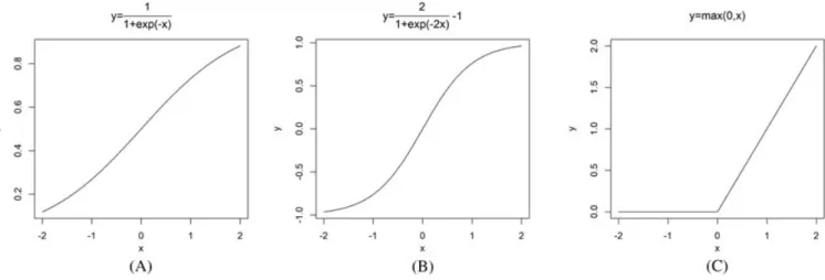
FIGURE 1 Activation functions. A, Sigmod function; B, Tanh function; C, Relu function

big health care data. It is based on a collection of connected units or nodes called artificial neurons or perceptrons. Often, neurons are organized in layers which consist of connections, each connection transferring the output of a neuronito the input of a neuronj.

There are some common components of neural network that are important for setting up the computation works. First, a so-called activation functionf(x)should be nonlinear, differentiable, and monotony. Commonly used activation functions include the Sigmod functionf(x) = 1∕(1 + e−x_{), the Tanh functionf(x) = 2sigmod (2x) − 1, and the Relu} functionf(x) = max(0,x). We display these functions in Figure 1.

Secondly, a loss functionl(y,y′_{)is specified to measure the loss of the true valueyand the predicted valuey}′_returned

from the functionf. For binary category outcome, we usually use the cross entropy14_{as the loss function.}

l(𝑦, 𝑦′) = −[𝑦 log(𝑦′) + (1−𝑦)log(1−𝑦′)] (5)

The model parameters in the networks may be estimated by minimizing the total loss function for all the samples. The computation can be carried out using the iterative gradient descent algorithms.

We may treat the multinomial logistic regression reviewed earlier as a special kind of deep learning method with only one layer. From Equation (2), we may find that the activation function for logistic regression is actually a generalization of the sigmod function, usually called softmax function

𝑓k(x) =softmaxk(x) = exp(𝛽T kx ) ∑M m=1exp ( 𝛽T mx ), k=1,…,M. (6)

For a general multicategory problem, the cross entropy loss function for a subject may be given as l(𝑦, 𝑦′) = − M ∑ m=1 𝑦mlog 𝑦′m, (7) where𝑦′

mis the predicted probability that the subject is in themth class based on the deep learning classifier. We next consider two specific deep learners that are now incorporated in standard softwares.

2.2.1

Multilayer perceptron

An MLP15_{is a class of feedforward ANN where connections between the units do not form a cycle. It can be viewed}

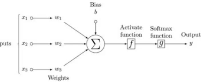
as a logistic regression classifier where the input is first transformed using a learned nonlinear transformationf. This transformation projects the input data into a space where it becomes linearly separable. Figure 2 provides the flow sheet of this approach.

To take a closer look at the structure, we may ignore the hidden layer and set the dimension of inputxito bep = 3 and show the single layer computation in Figure 3. Mathematically, a neuron in the(t + 1)th layerx(t + 1)is adjusted from x(t)via

x(t+1) =𝑓[b(t) +w(t)Tx(t)], (8) wherefis the activation function,b(t)is the so-called bias term at thetth layer, andw(t)is the weight vector of thetth layer.

FIGURE 2 Flowsheet of multilayer perceptron. Suppose the input isxi = (xi1,…,xi5). Each circle represents a neuron and each arrow is a connection between layers. The input layer consists of a set of neurons representing the input features. Each neuron in the hidden layer transforms the values from the previous layer with a weighted linear summation, followed by a nonlinear activation function. The output layer receives the values from the last hidden layer and such values are transformed into output values. The number of neurons in the output softmax layer is the same as the category numbers

FIGURE 3 Flowsheet of a simplified multilayer perceptron with one hidden layer. Suppose the input isxi = (xi1,xi2,xi3). The output of each neuron is calculated by a nonlinear functionfof the sum of its input plus a biasbas in Equation (8)

An MLP algorithm repeats the above calculation for a number of layers and stops at theTth layer. In the output layer or theTth layer, class-membership probabilities can be obtained from the softmax function.

The reason why MLP works well in practice is that it learns multiple levels of abstraction of data representations through multiple processing layers. The goal of representation learning or feature learning is to find an appropriate representation of data in order to perform a machine learning task. In particular, in MLP, each hidden layer maps its input data to an inner representation that tends to capture a higher level of abstraction. These learned features are increasingly more informative through layers toward the machine learning task. The backpropagation algorithm has a great significance during this process. We introduce a useful notation𝛿to represent the derivative of a loss function with respect to a dot product of weights and neurons. Then, backpropagation formula suggest that the value of𝛿for a particular hidden unit can be obtained by propagating the𝛿's backwards from units higher up in the network. Consequently, we can recursively calculate all the derivatives.

To train an MLP, we need to learn all the parameters of the model including the weightwand the biasb. The estimation is usually carried out under the stochastic gradient descent algorithm with minibatches.16_{Evaluating the gradients can be}

achieved through the backpropagation algorithm17_{(a special case of the chain rule of derivation). Software development}

for deep learning has been abundant and is rapidly evolving in the recent decade. In particular, open source libraries such asmxnetenable nonexperts to easily design, train, and implement deep neural networks. We will carry out all the computation in this paper usingmxnetsince it supports languages such asPythonorRand can train quickly on multiple GPUs. For more information about the software, visit https://mxnet.incubator.apache.org/index.html. We may download and installmxnetpackage using the following code. If there is an error about DiagrammeR during the installation, we recommend to manually install earlier version of DiagrammeR in advance.

In practice, the following operational parameters for the MLP need to be tuned by the user:

Layers.Number of layers and number of neurons in each layer. Usually, the number of neurons can be very large while the number of layers may be relatively moderate or small. The number of neurons in different layers may also differ.

Activation functions.Activation functions in each layer. All three functions in Figure 1 can be used while the Relu function is usually preferred for the simplicity of computation. For example, if we want to fill in two hidden layers, first containing 500 nodes and second containing 100 nodes, and choose both of the activation functions to be “Relu,” we can use the following function seriesmx.symbolfor specification.

Loss function. Loss function in the output layer. Usually, we choose the softmax function defined in Equation (6).

Number of round or epoch.The number of iterations over the sample data to train the model parameters. Often, we need very large number of round to achieve satisfactory numeric accuracy, similar to other nonlinear programming problems. One may specify the optionnum.roundin the software.

Learning rate.The step size in gradient descent method. This tuning parameter can be optimized via the cross validation. Alternatively, many practitioners recommended to use a small value such as 0.1 or 0.01. One may specify the option

learning.ratein the software.

Initializer.The initialization scheme for parameters, which specifies the unknown weight at the beginning, usually drawn from a uniform design. One may specify the optioninitializerin the software.

Array batch size.The batch size used for array training. The whole training data is usually divided into batches to facilitate the computing. For example, if we set 41 rounds, 40 batch size, 0.08 learning rate, uniform distribution (0.07) as the initial weight, we may use functionmx.model.FeedForward.createto create the following model specification.

Here, we need to encode the first level of y to be 1 and thus denote it as yy and we normalize each column of feature matrix d to obtain data matrix dd.

We use the previously constructed MLP symbol “softmax” as the input ofmx.model.FeedForward.create. It returns the fitted modelM1from which we can obtain the probability assessment matrix.

There is still limited discussion on how to set all these options to optimize the classification performance. Depending on the scale of the problem and complexity of the data, settings of real-world examples using MLP need to be addressed case by case.

After the model architectures are constructed and all the parameters are learned, every inputxican lead to a proba-bility vector of lengthMthrough the softmax loss. After such evaluation for all thensubjects, we obtain the probability assessment matrixp(1)as in the previous shallow learning methods.

2.2.2

Convolutional neural networks

Convolutional neural networks18_{(CNNs) are made up of neuron-like computational connections involving learnable}

weights and biases. Though the main hierarchical structures are similar to MLP, we highlight the following key differences.

First, the input for CNN are usually images or multidimensional data arrays rather than a vector in MLP. In fact, the overall learning process of CNN simulates the organization of the animal visual cortex. Thus, the layers of a CNN for a two-dimensional (2D) colored image typically have neurons arranged in 3 dimensions: width, height, and depth. The width and height can be the same as the dimension of the input image matrix. On the other hand, the depth would be 3 corresponding to Red, Green, and Blue channels for a colored 2D picture.

Secondly, we need three types of layers to build CNN architectures: the convolutional layer, the pooling layer (not always necessary to specify), and the fully connected layer that is the same as the hidden layer in MLP. The primary purpose of a convolutional layer is to detect distinctive local motif-like edges, lines, and other visual elements. Parameters including number of filters, their spatial extents, and stride should be specified. The pooling layer operates independently on every depth slice of the input and resizes it spatially, using the maximum (MAX) operation. For example, every MAX operation would be taking a max over 4 numbers if filter size is 2×2 with a stride of 2. Parameter such as filters sizes and stride should be settled at this stage. A CNN architecture contains a list of layers that transform the image volume into a probability vector. The initial volume stores the raw image pixels and the last volume stores the class risk scores.

To implement CNN, we may usemxnetpackage as well. There are a few key parameters to be specified by the user. The number of filters (or kernels) is the number of neurons, since each neuron performs a different convolution on the input to the layer (more precisely, the neurons' input weights form convolution kernels). Filter spatial extent is size of a filter (or a kernel). Usually, we use 3×3 kernel or 5×5 kernel. Every time, we will connect each neuron to a local region that is the kernel size of the input volume. We specify the stride with which we slide the filter. When the stride is 1, then we move the filters one pixel at a time. When the stride is 2, then the filters jump 2 pixels at a time as we slide them around, which will produce smaller output volumes spatially.

For example, suppose we want to fill in two convolution layer ensembles, first containing 20 filters and second con-taining 50 filters. Both of the activation functions are specified as “tanh.” Also, we use 5×5 kernel for convolution, 2×2 kernel for max pooling, and 2×2 stride for both of ensembles. After constructing convolution layer ensembles, we move on to construct one single fully connected layer with 500 hidden nodes and “tanh” to activate it. We can use function seriesmx.symbolto construct it as follows.

Other modeling options are similar to those for MLP discussed earlier. For example, if we specify 41 rounds, 40 batch size, 0.08 learning rate, uniform distribution (0.07) as the initial weight, we may use function mx.model. FeedForward.createto create the CNN model as follows.

We use the previously constructed CNN symbol “lenet” as the input ofmx.model.FeedForward.create. It returns the fitted modelM1that we can use to make classification. Every inputxican lead to a probability vector of lengthMafter the model architectures are constructed and the parameters are settled and learned. Computing such risk scores for all then objects, we may then obtain the probability assessment matrixp(1)for the downstream evaluation.

3

ACC U R AC Y M ET R I C S

All the learning methods reviewed in the preceding section will be examined by the accuracy metrics reviewed in this section. We provide a conceptual summary for each classification accuracy measure and introduce the associated soft-ware. These measures were originally proposed to assess the diagnostic accuracy of medical tests and widely adopted in epidemiology studies. We will see that they are equally applicable to evaluate classification accuracy for various learning methods.

3.1

Single model evaluation

First, we consider a few measures that are useful to describe the classification performance of a particular statistical model. For these measures, a greater value indicates a more satisfactory classification performance.

3.1.1

Hypervolume under the manifold

Hypervolume under the ROC manifold (HUM)19_{has been proposed as a generalization of AUC}1,2_{value for multicategory}

classification. Unlike the CCP to be defined in the next section, HUM does not depend on the class prevalence and thus reflects the intrinsic accuracy of the classifier.

We consider extending the definition of 2D ROC curve. Recall that a statistical learning method1 can generate a probability assessment vectorpi(1) = (pi1(1),…,piM(1))Tfor theith subject. To make classification decision, one may apply the following sequential thresholding rule: Ifpi1(1)> c1, then classify theith subject as class 1; otherwise,

ifpi2(1) > c2, then classify the subject as class 2; …; otherwise, ifpi,M−1(1) > cM−1, then classify the subject as

classM − 1; otherwise, classify as classM. WithMclasses, this procedure requiresM − 1 thresholdsc1,…,cM−1and

different threshold values produce different decision rules. At a fixed set ofM− 1 thresholds, the probability of correctly classifying themth class is denoted bytm(m = 1,…,M). For example,t1 = P(pi1(1)> c1|𝑦i = 1),t2 = P(pi1(1)≤ c1,pi2(1)>c2|𝑦i=2)and so forth. One plots(t1,t2,…,tM)inM-dimensional space for all decision rules (ie, all possible threshold values) and then connects these points to form an ROC manifold. WhenM = 2, t1 andt2 are simply the

sensitivity and specificity and the manifold reduces to the familiar ROC curve. WhenM = 3, the manifold reduces to the three-dimensional (3D) ROC surface. The ROC manifold itself may not be of much interest whenM ≥ 4. A more relevant quantity is the HUM that summarizes the overall accuracy for the model1.

Novoselova et al20_{developed anRpackageHUMthat can be directly downloaded from CRAN website. The}

correspond-ing Shiny web application (https://public.ostfalia.de/klawonn/HUM.htm) allows graphical display of 3D ROC surface. Figure 4 presents an example, displaying 3D view of three ROC surfaces, where we consider a leukemia data21_{to be}

described in Section 4.4 and plot the ROC manifolds for three selected genetic markers in the data. Clearly, the volume for the left panel is much greater than the other two panels, indicating the corresponding marker is a stronger classifier.

The aforementioned geometric definition of HUM may not be directly relevant to numerical evaluation. In fact, there is an appealing alternative probabilistic definition of HUM. Suppose there is a random sample involvingMsubjects and each subject is chosen from one of theMdistinct categories. Without loss of generality, we assume that themth subject is from themth category,m = 1,…,M. Then, HUM for a classification model1corresponds to the probability that all theMsubjects are correctly classified by the model1. WhenM = 2, we recall that AUC is the probability of correctly differentiating a pair of randomly chosen diseased and nondiseased subjects. Thus, HUM provides a direct generalization of AUC for multiple classes. The null value for HUM is 1∕M!and corresponds to a random guess.

The inference procedure for HUM has been discussed for ordered polychotomous responses19,22_{with a single marker}

(ie,p = 1). The calculation method has been implemented inRpackageHUM. For the more general case of unordered polychotomous responses and for model-based multivariate predictors (ie,p > 1), one needs to consider the methods in the work of Li and Fine.4_{The method is available inRpackagemccaand will be covered with details in this tutorial.}

FIGURE 4 Three-dimensional receiver operating characteristic surfaces for three gene expressions from leukemia data [Colour figure can be viewed at wileyonlinelibrary.com]

3.1.2

Correct classification probability

Another very popular multicategory classification accuracy measure is the CCP. To fix the notation, we write ̂𝑦i(1)to be the predicted class membership for theith subject using the machine learning model1. The CCP is thus defined to be the probability that the predicted class agrees with the true class for the subject

CCP=P(𝑦i= ̂𝑦i(1)). (9)

Using the law of total probability, the equation above can be rewritten as CCP= M ∑ m=1 P(̂𝑦i(1) =m|𝑦i=m)P(𝑦i=m) = M ∑ m=1 𝜌mP(̂𝑦i(1) =m|𝑦i=m), (10) where the probabilityP(̂𝑦i(1) =m|𝑦i=m)can be regarded as a class-specific CCP for themth category. WhenM = 2, the two class-specific CCP values are commonly referred to as the sensitivity and the specificity.1,2_{CCP directly assesses}

whether the mode-based classification for a subject is identical to his true class status. Its empirical version is simply the proportion of correctly classified subjects in the sample.

̂ CCP= 1 n n ∑ i=1 I(𝑦i= ̂𝑦(1)) (11)

Such a simple formula facilitates the application of CCP in many real problems, especially whenM is large. In fact, the computation time for CCP does not increase as the number of categories increases. CCP and its complement, misclassification rate, are commonly used in machine learning literature.

Machine classifiers usually output the probability assessment vectorp(1)directly and a decision-maker needs to take one more step to convert the probability into an actual class prediction ̂𝑦(1). In general, we may follow two types of decision rules to carry out the conversion.

The first type is the thresholding rule introduced in the preceding section. Based on such a rule, we may define the probability of correctly classifying themth class to betm =P(̂𝑦(1) =m|𝑦 =m),m = 1,…,M. The overall CCP for a model1is just a prevalence-weighted average

CCP=

M ∑ m=1

𝜌mtm. (12)

Besides the thresholding rule, we note thattmmay also be defined without using any threshold. In fact, we may consider the take-the-winner rule: Recall that a classifier1generates a probability assessment vectorpi(1) = (pi1(1), …, piM(1))T for theith subject. Decision-makers may assign a subject to one of theMcategories according to the greatest component in the probability vectorpi(1). Under this rule, we may obtain for themth class

We note that, whenM = 2, thresholding rule and take-the-winner rule yield the same definition oft1andt2(sensitivity

and specificity).1,2

Though it provides a straightforward assessment on the performance of a fixed sample, the estimated overall CCP value is quite sensitive to the distribution of different classes in the particular data sample and thus cannot lend support to external validity for some studies where prevalence information is unavailable. For example, CCP values obtained for low-risk disease groups may be dominated by the specificity.

The implementation of CCP is quite easy after a classification is done. We will use the functionCCPinRpackagemcca in the following illustration.

3.1.3

R-squared value

R-squared (RSQ) value23-26_{also called a coefficient of determination, is extensively studied in linear regression and has}

been discussed for binary logistic regression models. Simply speaking, the value ofR2is the fraction of the total variance of the response (continuous or categorical) explained by the model. A greater percentage of RSQ value may indicate that a higher proportion of the variation of the response may be attributable to the markers included in the model and the classification based on such a model may thus lead to more meaningful results. The estimated RSQ value, though not directly rating the accuracy of classification, is still considered an important model evaluation statistic. There is also no probabilistic interpretation for RSQ value even though it lies between 0 and 1.

For themth class, the RSQ value3_{for a particular model}1_{is defined as}

R2m= var(𝛿m) −E(var(𝛿m|1)) var(𝛿m) = var(pim) 𝜌m(1−𝜌m) , (14)

where the second equality follows asE(Yi = m|1) = pim(1), andpimis themth element of the probability vector p_i(1)defined earlier. The overall RSQ value is simply an average of the class-specific RSQ values

RSQ= 1 M M ∑ m=1 R2 m. (15)

The applications ofR2for multicategory classification is not as common as the two measures in the preceding sections in practice, mainly because it is not widely regarded as an accuracy measure but a model fitting summary statistic. It has recently attracted more attention from biostatistical researchers due to its close connection to the IDI.3_{The computation}

of multiclass RSQ is implemented in functionRSQinRpackagemcca.

3.1.4

Polytomous discrimination index

Polytomous discrimination index (PDI)5,27,28_{is a recently proposed diagnostic accuracy measure for multicategory}

classifi-cation. Similar to HUM, PDI is also evaluating the probability of an event related to simultaneously classifyingMsubjects fromMcategories. While HUM is pertaining to the event that allMsubjects are correctly identified to their correspond-ing categories, PDI is pertaincorrespond-ing to the number of subjects in the set ofMsubjects that are correctly identified to his/her category.

To define the PDI, we consider a random sample that involvesMsubjects and each subject is chosen from one of theM distinct categories. Without loss of generality, we assume that theith subject is from theith category. The classification decision is achieved via a joint comparison of theMsubjects. Using earlier notations, for a classification model1, we may denote the probability of placing a subject from categoryiinto categoryjbypi𝑗(1). A classisubject can be correctly classified ifpii(1)>p𝑗i(1)for allj ≠ i. For a fixed categoryi, we may define the class-specific PDI to be

PDIi=p(pii(1)>p𝑗i(1) 𝑗≠i|𝑦i=i) (16) and the overall PDI to be

PDI= 1 M M ∑ m=1 PDIm. (17)

WhenM = 2, PDI also reduces to AUC and thus can be viewed as a generalization of AUC for the multiclass problem. However, whenM ≥ 3, PDI value is always greater than HUM for a classifier1. Models or diagnostic biomarkers with poor PDI values usually also have poor HUM values. The lower bound for PDI is 1∕M, corresponding to random guess.

PDI is not as widely applied as HUM and CCP to assess the diagnostic and classification accuracy. We suggest its value should also be reported along with other major accuracy measures. Specifically, we would recommend computing PDI for big data studies and screen out unnecessary biomarkers whose PDI values are below a satisfactory level. The computation of PDI is implemented in functionPDIinRpackagemcca.

3.2

Model comparison

When comparing two models used to make prediction or classification for the same data, it is usually not advisable to only check the difference of a single accuracy measure. For example, it is noted by many authors that the difference of HUM between two models may not be informative when the baseline model is already quite accurate. We next consider two more appropriate measures for comparing two models.

We need more notations. Now, suppose that in addition to model1introduced earlier, more variable(s) are included and we construct a model2 that is based on a set of predictorsΩ2 ⊃ Ω1. We use the nested-structure notations as

they are widely discussed in the literature. We note that there are studies where the accuracy improvement occurs among nonnested models as well. Our proposed methods can apply with slight modification. The newly constructed model2 generates another probability vectorpi(2) = (pi1(2),…,piM(2))for theith subject.

3.2.1

Net reclassification improvement

Net reclassification improvement (NRI)29_{is a numeric characterizations of accuracy improvement for diagnostic tests or}

classification models and were shown to have certain advantage over analyses based on ROC curves.

While ROC-based measures have been widely adopted, it has been argued by many authors30_{that such measures may}

not be good criteria to quantify improvements in diagnostic or classification accuracy when the added value of a new predictor to an existing model is of interest. NRI can address these limitations since it essentially calculates the increase in correct classification between models.

The multicategory NRI from a baseline model1to a more complicated model2is NRI=

M ∑ m=1

𝜌m{CCPm(2) −CCPm(1)}. (18)

NRI directly reflects how often the new model corrects the incorrectly classified cases in the old model and is therefore very appealing to practitioners. We note another interpretation for NRI is the difference of Youden's index of the two models. For additional discussion of these recent developments, we refer the reader to other reference materials.31-34_{We note}

that these metrics provide different perspectives for accuracy studies and there are also critiques in the literature (see, for example, the works of Pepe et al,35_{Hilden and Gerds,}36_{and Kerr et al}37_{). In particular, Hilden and Gerds}36_pointed

out that NRI sometimes may inflate the prognostic performance of added biomarkers, and Kerr et al37_{argued that NRI}

may perform poorly under some nonlinear data generating mechanisms. Thus, users of such popular metrics should also exercise caution in practice.

The computation of multiclass NRI is implemented in functionNRIinRpackagemcca. There are also a few other packages that allow the calculation of different versions of NRI.

3.2.2

Integrated discrimination improvement

Integrated discrimination improvement (IDI)35_{is originally defined as the improvement of the integration for sensitivity}

and specificity over all thresholds for binary classification. Recently, it has been extended to multiclass version by noting its strong connection to RSQ values.23,24,26,29 In fact, IDI may be regarded simply as the increase inR2 defined in (15). Specifically, we define the multiclass IDI to be

IDI= 1 M M ∑ m=1 ( R2m(2) −R2m(1) ) . (19)

IDI thus reflects how many more percentage of variation of the multiclass response the new model explains. Unlike NRI, this metric does not correspond to a probability of a random event and thus has no probabilistic interpretation. However, the IDI value certainly indicates the added explanation power of the new model relative to the old model and therefore also widely adopted in biomedical studies. In the literature, IDI has the same critique as the NRI,38_{and we suggest practitioners}

to use these improvement measures with caution.

The computation of multiclass IDI is implemented in functionIDIinRpackagemcca. There are also a few other packages that allow the calculation of different versions of IDI.

4

C A S E ST U D I E S

In this tutorial, we useRas the programming language. In order to analyze all the following examples, we needmcca

package that is specifically constructed for multicategory classification accuracy. It contains functions to evaluate the six accuracy methods introduced in Section 3 for binary and multicategory classifiers. It can be download directly from CRAN website https://CRAN.R-project.org/package=mcca.

4.1

Guideline

In this section, we provide a step-by-step guideline on how to analyze the classification accuracy for a real data set. We first consider a single model evaluation. The following is the general procedure.

Single model evaluation:

Step 1 First, we pre-process the raw data. After downloading data to the computer, we clean the data by removing or imputing missing entries. We then form a data matrix ofp + 1 columns includingpcolumns of the predictor features and 1 column of theM-class response.

Step 2 Then, we may divide the whole dataset randomly into two parts: a training data and a test data. We use the training data to build the statistical model and the test data to assess the out-of-sample performance.

Step 3 For single model evaluation, we choose one set of predictorsΩ1and build a statistical model based on these

variables. The statistical model can be based on any of the shallow learning methods (multinomial logistic regression, classification tree, SVM, or LDA) or the deep learning methods (MLP or CNN). Pay attention that some of the procedures require sophisticated parameters tuning to arrive at a satisfactory model.

Step 4 After the model is built, we apply this model to training and test data, respectively, to obtain the in-sample and out-of-sample performance assessment. As discussed in Section 2, we may obtain a probability assessment matrix from the fitted model and make classification decision based on the risk scores. Thus, we may feed this matrix into the accuracy methods CCP, PDI, RSQ, HUM reviewed in Section 3 and obtain the accuracy metric values accord ingly.

When the goal is to evaluate the accuracy improvement, we need to consider two models with different degree of complexity. In this tutorial, we mainly consider two nested models built from the same learning program where the simpler model can be reduced from the more complex model. In general, our discussion can also be applied to any two classification models with nonnested structure. We provide a simple guideline on paired model comparison in the following.

Model comparison:

Step 1 First, we pre-process the data as in the single model evaluation and divide the whole data into training and test sets. For paired model comparison, we choose two sets of predictorsΩ1andΩ2. We aim to evaluate the

improvement of the model constructed by the two sets of predictors.

Step 2 We then use either a shallow learning or a deep learning method to train the statistical model for both sets of predictors, separately. Consequently, we arrive at two models1and2, based onΩ1andΩ2, respectively.

Step 3 After the models are built, we apply the two fitted models to training and test data to obtain the in-sample and out-of-sample performance assessment. As discussed in Section 2, we may obtain probability assessment

matrices for the two models and make classification decision accordingly. We may then compute NRI and IDI reviewed in Section 3 and interpret the values accordingly.

In the followingRillustration, one only needs to specify the two setsΩ1andΩ2to acquire the training set accuracy. To

compute the test set accuracy, one needs to explicitly extract the probability matrix from the fitted models and then feed such a matrix to theRfunctions.

4.2

Breast cancer

Breast cancer is the most common cancer and the second greatest cause of cancer mortality for women. The diagnostic sys-tem at University of Wisconsin Hospitals analyzed digital morphometry samples from 569 patients where 212 malignant cases were identified. We revisit this Wisconsin breast cancer data that is publicly available at the UCI website:

https∶ ∕∕archive.ics.uci.edu∕ml∕datasets∕.

Features are computed from a digitized image of a fine needle aspirate of a breast mass. These measurements describe characteristics of the cell nuclei present in the image. The dataset contains 30 real-valued features computed for cell nucleus. The diagnosis outcome is either malignant or benign. Each input variable represents certain feature of the cell nucleus such as radius, perimeter, area, smoothness, concavity, and symmetry. These real values are standardized before the deep learning calculation.

Following the guideline given in the preceding section, we carry out the following step-by-step calculation to this dataset.

Step 1 Check whether the dataset is appropriate. After we download the dataset from UCI website, we save the file

wpbc.datato the desktop. Then, we assign proper variable names for the data file.

After the above operation, we obtain a data file with 194 observations and 34 variables where the first column is the binary outcome variable indicating the disease status.

Step 2 We consider a sample with only the first ten variables (Outcome,Time,radius MEAN, texture MEAN,

perimeter MEAN, etc) in the original data file. Then, we randomly split this data frame into training and test data in a 2∶1 ratio.

Step 3 Carry out the classification procedure and evaluate the accuracy measures. One may simply choose a func-tion for the accuracy evaluafunc-tion methods (hum, ccp, rsq, pdi) with an option method specifying

˜prob˜, corresponding respectively to multinomial logistic regression, decision tree, linear discrimination analysis, SVM, and arbitrary probability assessment matrix obtained externally. The following code is to evaluate HUM of a multinomial logistic regression and RSQ value of a decision tree for the training data created before.

In this case, using logistic regression achieves over 79% HUM value, suggesting that the two disease categories can be differentiated by the markers with a moderately high probability.

The above code computes the standard error and 95% confidence interval for HUM value using the boot-strap method.

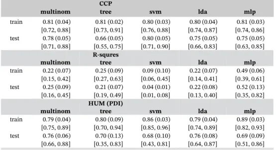
All accuracy measures for the training sample and the test sample are summarized in Table 1 along with their standard errors and 95% confidence intervals. We notice that in-sample accuracy is usually higher than the out-of-sample accuracy. In particular, MLP attains the top in-sample accuracy among all classification methods under all the four evaluation criteria.

To evaluate the accuracy for the test sample, one needs to carry out the model fitting explicitly and generate the probability assessment matrix for the test sample. The following is an example to obtain the probability assessment matrix for the test sample when using a multinomial logistic regression model.

TABLE 1 Accuracy for training and test samples for breast cancer data along with their standard errors (in the parenthesis) and 95% confidence intervals (in the brackets)

CCP

multinom tree svm lda mlp

train 0.81 (0.04) 0.81 (0.02) 0.80 (0.03) 0.80 (0.04) 0.81 (0.03) [0.72, 0.88] [0.73, 0.91] [0.76, 0.88] [0.74, 0.87] [0.74, 0.86] test 0.78 (0.05) 0.66 (0.05) 0.80 (0.05) 0.75 (0.05) 0.75 (0.05) [0.71, 0.88] [0.55, 0.75] [0.71, 0.90] [0.66, 0.83] [0.63, 0.85]

R-squres

multinom tree svm lda mlp

train 0.22 (0.07) 0.25 (0.09) 0.09 (0.10) 0.22 (0.07) 0.49 (0.06) [0.15, 0.42] [0.27, 0.63] [0.06, 0.45] [0.14, 0.41] [0.39, 0.61] test 0.25 (0.09) 0.21 (0.07) 0.04 (0.01) 0.22 (0.08) 0.52 (0.13) [0.16, 0.45] [0.19, 0.49] [0.01, 0.08] [0.13, 0.40] [0.35, 0.82]

HUM (PDI)

multinom tree svm lda mlp

train 0.79 (0.04) 0.80 (0.09) 0.86 (0.03) 0.79 (0.04) 0.89 (0.03) [0.75, 0.89] [0.70, 0.94] [0.85, 0.96] [0.74, 0.89] [0.82, 0.93] test 0.76 (0.06) 0.70 (0.13) 0.68 (0.10) 0.76 (0.08) 0.69 (0.09) [0.66, 0.88] [0.35, 0.83] [0.43, 0.81] [0.64, 0.87] [0.51, 0.86] Abbreviations: CCP, correct classification probability; HUM, hypervolume under the ROC manifold; PDI, polytomous discrimination index.

After the probability assessment matrixpm2_mis obtained, we may then evaluate the accuracy measure such as the HUM as follows.

The HUM for this model is 0.765 with a standard error 0.062. The 95% confidence interval for HUM is

[0.657,0.876].

We provide more details on the implementation of MLP method. In this example, we use two hidden lay-ers with 50 and 10 nodes, respectively. The activation function is chosen to be the Relu function. We specify learning.rate=0.08, batch.size=40, num.round=40. The following code specifies the necessary symbol for MLP computing and implements the multilayer model fitting.

After the abovemodelis fitted using MLP method, we may then extract the probability assessment matrixpp as follows. The accuracy measures such as CCP and HUM can be computed accordingly for the training sample and the test sample.

For the test sample, we can feed the fittedmodelinto the predict function to obtain the probability assessment matrixpm2_mlpand then evaluate the test accuracy using functions such ashum.

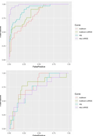
In this caseM = 2, the ROC manifold is actually a 2D ROC curve for each classifier. We plot the ROC curves of the five classifiers in Figure 5 for training (top) and test (bottom) data, respectively. We observe that MLP outperforms other classifiers for the training sample while its performance is not as good as LDA for the test sample.

Step 4 We now consider an accuracy improvement study and compare models based on the above dataset with a larger data containing from 23rd to 27th variables on top of the first nine markers. We usemydatalto represent the new dataset in the following.

FIGURE 5 Receiver operating characteristic curve of five classifiers for training (top) and test (bottom) data [Colour figure can be viewed at wileyonlinelibrary.com]

We may then evaluate the accuracy improvement for the training data. We exemplify the calculation by setting the shallow learning classifier to be multinomial logistic regression. Other classification methods can be used by changing themethodoption in the followingnriandidifunctions.

The test sample can be similarly evaluated using the following code.

We next consider the deep learning classifier MLP. Using the same model settings as in Step 3, we apply the following code to obtain the IDI and NRI values for the accuracy improvement using MLP.

FIGURE 6 Receiver operating characteristic curves for training (top) and test (bottom) data. Curves “multinom” and “mlp” are for the baseline model and curves “multinom LARGE” and “mlp LARGE” are for the model with additional markers [Colour figure can be viewed at wileyonlinelibrary.com]

FIGURE 7 Net reclassification improvement (NRI) and integrated discrimination improvement (IDI) values for all the five machine learning models to predict the breast cancer outcomes: multinomial logistic regression, tree, support vector machine (SVM), linear discriminant analysis (LDA), and multilayer perceptron (MLP). The left panel is for the training dataset while the right panel is for the test dataset. The baseline model contains nine markers and the new model contains five more genes [Colour figure can be viewed at

wileyonlinelibrary.com]

Figure 6 plots the ROC curves of small and large dataset using training and test data, respectively. One can observe that switching from the smaller set to the larger set leads to a slightly higher ROC curve for the multinomial logistic regression and the MLP method.

4.3

Leukemia

We next consider an example withM = 3 categories. Golub et al21_{analyzed a leukemia dataset using microarray gene}

expression. The data included three types of acute leukemias: acute lymphoblastic leukemia arising from T-cells (ALL T-cell), acute lymphoblastic leukemia arising from B-cells (ALL B-cell), and acute myeloid leukemia (AML). The dataset contains 8 ALL T-cell samples, 19 ALL B-cell samples, and 11 AML samples. Each sample contains 3916 gene expression values obtained from Affymetrix high-density oligonucleotide microarrays. The dataset to be analyzed is downloaded from http://www.broad.mit.edu/cgi-bin/cancer/datasets.cgi.

The training and test data were prepared by the authors in this case and we will thus use these data directly.

Step 1 Input the training data. In this case, we only consider six gene expression for the simplicity and therefore attain a training data with 38 subjects and 7 variables. The first columnstindicates the three types of disease status

ALLb, ALLt, AML.

Step 2 Input the test data in the same way. These 35 subjects were used by Golub et al as the test samples and we thus follow the same analysis as the original authors.

Step 3 We construct a baseline model with the first four gene expressions. We used similarRcode as in the preceding section except that we need to set the number of outcomek=3in all the functions. We use the following code to compute HUM for a multinomial logistic regression model and RSQ value for a tree model. Other accuracy measures for all kinds of classifiers can be similarly obtained.

We next illustrate the deep learning computation using MLP. In this case, we set the number output nodes to be 3 for the three-category classification.

After the model is fitted with the above procedure, we may then obtain the probability assessment matrix and evaluate the accuracy measures using the following code.

Test sample can be similarly evaluated using the following code.

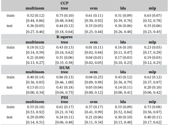
Accuracy measures for all the classifiers are reported in Table 2 along with their standard errors (in the parenthesis) and 95% confidence intervals (in the brackets). In this example, tree method attains the best in-sample classification accuracy. For example, applying tree method to the four selected gene expression, we can

TABLE 2 Accuracy for training and test samples in Leukemia data along with their standard errors (in the parenthesis) and 95% confidence intervals (in the brackets)

CCP

multinom tree svm lda mlp

train 0.52 (0.12) 0.75 (0.10) 0.61 (0.11) 0.51 (0.09) 0.65 (0.07) [0.44, 0.86] [0.48, 0.84] [0.50, 0.92] [0.39, 0.76] [0.52, 0.78] test 0.36 (0.05) 0.44 (0.12) 0.35 (0.05) 0.36 (0.06) 0.35 (0.06) [0.27, 0.46] [0.18, 0.64] [0.25, 0.44] [0.26, 0.48] [0.23, 0.45]

R-squres

multinom tree svm lda mlp

train 0.18 (0.12) 0.43 (0.13) 0.01 (0.11) 0.16 (0.10) 0.23 (0.03) [0.14, 0.59] [0.16, 0.62] [0.02, 0.44] [0.11, 0.47] [0.17, 0.29] test 0.21 (0.04) 0.51 (0.06) 0.04 (0.01) 0.17 (0.03) 0.19 (0.03) [0.13, 0.27] [0.35, 0.58] [0.02, 0.05] [0.10, 0.23] [0.12, 0.25]

HUM

multinom tree svm lda mlp

train 0.40 (0.14) 0.86 (0.13) 0.04 (0.25) 0.43 (0.12) 0.62 (0.12) [0.36, 0.85] [0.46, 1.00] [0.09, 0.98] [0.36, 0.79] [0.37, 0.87] test 0.13 (0.11) 0.41 (0.18) 0.05 (0.04) 0.14 (0.11) 0.20 (0.10) [0.00, 0.34] [0.04, 0.75] [0.00, 0.12] [0.00, 0.41] [0.06, 0.42]

PDI

multinom tree svm lda mlp

train 0.55 (0.10) 0.61 (0.17) 0.37 (0.17) 0.55 (0.09) 0.73 (0.08) [0.53, 0.92] [0.21, 0.74] [0.41, 0.99] [0.52, 0.84] [0.56, 0.87] test 0.29 (0.09) 0.24 (0.11) 0.21 (0.06) 0.30 (0.10) 0.40 (0.11) [0.14, 0.51] [0.06, 0.48] [0.11, 0.34] [0.15, 0.48] [0.17, 0.62] Abbreviations: CCP, correct classification probability; HUM, hypervolume under the ROC manifold; PDI, polyto-mous discrimination index.

differentiate the three types of tumors with a 86% probability according to the reported HUM value. The out-of-sample performance is much worse for all methods, mainly due to the small sample size.

Step 4 We then compare the above models with more complicated models involving additional markers. To this end, we include two more genetic biomarkers from the data file.

We first evaluate NRI and IDI for multinomial logistic regression models, comparing the model with four markers and the model with six markers.

We next consider evaluating NRI and IDI for deep learning classifier MLP.

4.4

ADHD data

Next, we analyze the attention deficit hyperactivity disorder (ADHD) data from the ADHD-200 Sample Initiative (https:// fcon1000.projects:nitrc:org_indi_adhd200). ADHD is a common childhood disorder and can continue through adoles-cence and adulthood. Symptoms include difficulty in staying focused and paying attention, difficulty in controlling behavior, and overactivity. The dataset that we used is part of the ADHD-200 Global Competition datasets and can be requested from the ADHD website for research purpose. It consists of 406 subjects, with 221 normal controls and 185 combined ADHD subjects.

Resting state fMRIs and T1-weighted images were acquired for each subject. RAVENS methodology is based on a volume-preserving spatial transformation. Figures 8 and 9 display two typical individuals where the first row is an ADHD patient and the second row is a normal control. The learning task is then to differentiate the two types of patients using the complicated neural image data.

In this case, it is infeasible to run any of the shallow learning classifier directly on the image input. The classification is achieved with CNN introduced earlier. For this example, the input data tensorAis of dimension 160 × 160 × 128,

FIGURE 8 Axial, Sagittal, Coronal view at the center of the brain MRI for two selected subjects, one with AD (1st row) and one without AD (2nd row) [Colour figure can be viewed at wileyonlinelibrary.com]

FIGURE 9 MRI images for two selected brains, one with AD (1st row) and one without AD (2nd row) [Colour figure can be viewed at wileyonlinelibrary.com]

which can be viewed as a stack of 160 by 160 size images with channel equal to 128. We apply different kernels of sizes 2 ×2 ×128, 3 ×3 × 128, and 4 × 4 ×128, respectively. The pooling layers in the CNN model are all 2 × 2Pool2.

The calculation is implemented using themxnetpackage inR. First, we need to prepare the data in an appropriate format to be loaded into the training network. The raw image data are stored in NIfTI form under two folders for AD and NC, respectively, and can be read inRusing f1unctionreadNIfTIfrom libraryoro.nifti.

We arrive at a list objectbiglistincluding both AD and NC subjects. The above code also randomly split the whole data into a training set (n = 300) and a test set (n = 106). The data to be fed into the CNN algorithm is a four-dimensional array, with the first three dimensions defining the size of the tensor images and the last dimension being the sample size. Next, we create the network structure as follows.

The above construction of the network withmxnetinRis lengthy but intuitive, like other deep learning approaches. Typereluforces all the negative value to zero, providing relatively faster training speed thansigmoidortanhfunction. In the pooling function, we have a parameterstridethat defines how the sliding window on each layer is moving on both horizontal and vertical directions.

We specify the device for the training method to be GPU withdevice <- mx.gpu()command. Note that, to facil-itate the graphical computing, the user's graphic card needs to support CUDA and has the CUDA Toolkit installed. Otherwise, only CPU is supported and this line of code needs to be modified asdevice <- mx.cpu().

After the model is trained, we may use the trained classifier to predict the test data.

FrompredictProb, one can obtain the predicted probabilities and we can further calculate accuracy measures such

as HUM and CCR. Such computation can be done in the same manner as in the previous two examples and we do not repeat the evaluation in this tutorial for space consideration.

AC K N OW L E D G E M E N T S

We thank Adrian Roellin for helpful comments that improve the clarity of the presentation on deep learning. This work was partly supported through the Academic Research Funds R-155-000-205-114 and R-155-000-195-114 and through the Tier 2 MOE funds in Singapore MOE2017-T2-2-082: R-155-000-197-112 (Direct cost) and R-155-000-197-113 (IRC).

CO N F L I CT O F I N T E R E ST

The authors declare no potential conflict of interests.

F I NA N C I A L D I S C LO S U R E

None reported.

O RC I D

Jialiang Li https://orcid.org/0000-0002-9704-4135 R E F E R E N C E S

1. Zhou X-H, Obuchowski NA, McClish DK.Statistical Methods in Diagnostic Medicine. New York, NY: John Wiley & Sons; 2002. 2. Pepe MS.The Statistical Evaluation of Medical Tests for Classification and Prediction. Oxford, UK: Oxford University Press; 2003. 3. Li J, Jiang B, Fine JP. Multicategory reclassification statistics for assessing improvements in diagnostic accuracy. Biostatistics.

2013;14(2):382-394.

4. Li J, Fine JP. ROC analysis with multiple classes and multiple tests: methodology and its application in microarray studies.Biostatistics. 2008;9(3):566-576.

5. Van Calster B, Vergouwe Y, Looman CWN, Van Belle V, Timmerman D, Steyerberg EW. Assessing the discriminative ability of risk models for more than two outcome categories.Eur J Epidemiol. 2012;27(10):761-770.

6. Kwak C, Clayton-Matthews A. Multinomial logistic regression.Nursing Research. 2002;51(6):404-410. 7. Vapnik V.Statistical Learning Theory. New York, NY: Wiley; 1998.

8. Suykens JAK, Vandewalle J. Least squares support vector machine classifiers.Neural Process Lett. 1999;9(3):293-300.

9. Crammer K, Singer Y. On the algorithmic implementation of multiclass kernel-based vector machines.J Mach Learn Res. 2001;2:265-292. 10. Lee Y, Lin Y, Wahba G. Multicategory support vector machines, theory, and application to the classification of microarray data and satellite

radiance data.J Am Stat Assoc. 2004;99(465):67-81.

11. Liaw A, Wiener M. Classification and regression by randomforest.R News. 2002;2(3):18-22.

12. Mika S, Ratsch G, Weston J, Scholkopf B, Mullers KR. Fisher discriminant analysis with kernels. In: Neural Networks for Signal Processing IX: Proceedings of the 1999 IEEE Signal Processing Society Workshop; 1999; Madison, WI.

13. Schalkoff RJ.Artificial Neural Networks. Vol 1. New York, NY: McGraw-Hill; 1997.

14. Shore J, Johnson R. Axiomatic derivation of the principle of maximum entropy and the principle of minimum cross-entropy.IEEE Trans Inf Theory. 1980;26(1):26-37.

15. Gardner MW, Dorling SR. Artificial neural networks (the multilayer perceptron)—a review of applications in the atmospheric sciences.

Atmospheric Environment. 1998;32(14-15):2627-2636.

16. Zhao K, Huang L. Minibatch and parallelization for online large margin structured learning. In: Proceedings of the 2013 Conference of the North American Chapter of the Association for Computational Linguistics: Human Language Technologies; 2013; Atlanta, GA. 17. Hecht-Nielsen R. Theory of the backpropagation neural network.Neural Networks. 1988;1(1):445-448.

18. Krizhevsky A, Sutskever I, Hinton GE. Imagenet classification with deep convolutional neural networks. In: Advances in Neural Information Processing Systems 25 (NIPS Proceedings); 2012.

19. Li J, Chow Y, Wong WK, Wong TY. Sorting multiple classes in multi-dimensional ROC analysis: parametric and nonparametric approaches.Biomarkers. 2014;19(1):1-8.

20. Novoselova N, Beffa CD, Wang J, et al. HUM calculator and HUM package for R: easy-to-use software tools for multicategory receiver operating characteristic analysis.Bioinformatics. 2014;30(11):1635.

21. Golub TR, Slonim DK, Tamayo P, et al. Molecular classification of cancer: class discovery and class prediction by gene expression monitoring.Science. 1999;286:531-537.

22. Nakas CT, Yiannoutsos CT. Ordered multiple-class ROC analysis with continuous measurements.Statist Med. 2004;23(22):3437-3449. 23. Cox DR, Wermuth N. A comment on the coefficient of determination for binary response.Am Stat. 1992;46(1):1-4.

24. Menard S. Coefficients of determination for multiple logistic regression analysis.Am Stat. 2000;54(1):17-24. 25. Hu B, Palta M, Shao J. Properties ofR2_{statistics for logistic regression.Statist Med. 2006;25(8):1383-1395.}

26. Tjur T. Coefficients of determination in logistic regression models—a new proposal: the coefficient of discrimination. Am Stat. 2009;63(4):366-372.

27. Van Calster B, Van Belle V, Vergouwe Y, Timmerman D, Van Huffel S, Steyerberg EW. Extending thec-statistic to nominal polytomous outcomes: The polytomous discrimination index.Statist Med. 2012;31(23):2610-2626.

28. Li J, Feng Q, Fine JP, Pencina MJ, Van Calster B. Nonparametric estimation and inference for polytomous discrimination index.Stat Methods Med Res. 2017:0962280217692830.

29. Pencina MJ, D'Agostino RB Sr, D'Agostino RB, Vasan RS Jr. Evaluating the added predictive ability of a new marker: from area under the ROC curve to reclassification and beyond.Statist Med. 2008;27(2):157-172.

30. Pepe MS, Janes H, Longton G, Leisenring W, Newcomb P. Limitations of the odds ratio in gauging the performance of a diagnostic, prognostic, or screening marker.Am J Epidemiol. 2004;159(9):882-890.

31. Steyerberg EW, Vickers AJ, Cook NR, et al. Assessing the performance of prediction models, a framework for traditional and novel measures.Epidemiology. 2010;21(1):128-138.

32. Pencina MJ, D'Agostino RB Sr, Steyerberg EW. Extensions of net reclassification improvement calculations to measure usefulness of new biomarkers.Statist