Abstract
This paper describes a system for the evolution and co-evolution of virtual creatures that compete in physically simulated three-dimensional worlds. Pairs of individuals enter one-on-one contests in which they contend to gain control of a common resource. The winners receive higher relative fitness scores allowing them to survive and reproduce. Realistic dynamics simulation including gravity, collisions, and friction, restricts the actions to physically plausi-ble behaviors.
The morphology of these creatures and the neural systems for controlling their muscle forces are both genetically determined, and the morphology and behavior can adapt to each other as they evolve simultaneously. The genotypes are structured as directed graphs of nodes and connections, and they can efficiently but flexibly describe instructions for the development of creatures’ bodies and control sys-tems with repeating or recursive components. When simulated evolutions are performed with populations of competing creatures, interesting and diverse strate-gies and counter-stratestrate-gies emerge.
1 Introduction
Interactions between evolving organisms are generally believed to have a strong influence on their resulting com-plexity and diversity. In natural evolutionary systems the measure of fitness is not constant: the reproducibility of an organism depends on many environmental factors including other evolving organisms, and is continuously in flux. Com-petition between organisms is thought to play a significant role in preventing static fitness landscapes and sustaining evolutionary change.
These effects are a distinguishing difference between natural evolution and optimization. Evolution proceeds with no explicit goal, but optimization, including the genetic algo-rithm, usually aims to search for individuals with the highest possible fitness values where the fitness measure has been predefined, remains constant, and depends only on the indi-vidual being tested.
The work presented here takes the former approach. The fitness of an individual is highly dependent on the specific behaviors of other individuals currently in the population. The hope is that virtual creatures with higher complexity and more interesting behavior will evolve than when applying the selection pressures of optimization alone.
Many simulations of co-evolving populations have been performed which involve competing individuals [1,2]. As examples, Lindgren has studied the evolutionary dynamics of competing game strategy rules [14], Hillis has demon-strated that co-evolving parasites can enhance evolutionary optimization [9], and Reynolds evolves vehicles for compe-tition in the game of tag [19]. The work presented here involves similar evolutionary dynamics to help achieve interesting results when phenotypes have three-dimensional bodies and compete in physically simulated worlds.
In several cases, optimization has been used to automat-ically generate dynamic control systems for given two-dimensional articulated structures: de Garis has evolved weight values for neural networks [6], Ngo and Marks have applied genetic algorithms to generate stimulus-response pairs [16], and van de Panne and Fiume have optimized sen-sor-actuator networks [17]. Each of these methods has resulted in successful locomotion of two-dimensional stick figures.
The work presented here is related to these projects, but differs in several respects. Previously, control systems were generated for fixed structures that were user-designed, but here entire creatures are evolved: the evolution determines the creature morphologies as well as their control systems. The physical structure of a creature can adapt to its control system, and vice versa, as they evolve together. Also, here the creatures’ bodies are three-dimensional and fully physi-cally based. In addition, a developmental process is used to generate the creatures and their control systems, and allows similar components including their local neural circuitry to be defined once and then replicated, instead of requiring each to be separately specified. This approach is related to L-systems, graftal grammars, and object instancing techniques [8,11,13,15,23]. Finally, the previous work on articulated structures relies only on optimization, and competitions between individuals were not considered.
Evolving 3D Morphology and Behavior by Competition
Karl Sims
Thinking Machines Corporation
(No longer there)
A different version of the system described here has also been used to generate virtual creatures by optimizing for spe-cific defined behaviors such as swimming, walking, and fol-lowing [22].
Genotypes used in simulated evolutions and genetic algorithms have traditionally consisted of strings of binary digits [7,10]. Variable length genotypes such as hierarchical Lisp expressions or other computer programs can be useful in expanding the set of possible results beyond a predefined genetic space of fixed dimensions. Genetic languages such as these allow new parameters and new dimensions to be added to the genetic space as an evolution proceeds, and therefore define rather a hyperspace of possible results. This approach has been used to genetically program solutions to a variety of problems [3,12], as well as to explore procedurally generated images and dynamical systems [20,21].
In the spirit of unbounded genetic languages, directed
graphs are presented here as an appropriate basis for a
gram-mar that can be used to describe both the morphology and neural systems of virtual creatures. The level of complexity is variable for both genotype and phenotype. New features and functions can be added to creatures or existing ones removed, as they evolve.
The next section of this paper describes the environment of the simulated contest and how the competitors are scored. Section 3 discusses different simplified competition patterns for approximating competitive environments. Sections 4 and 5 present the genetic language that is used to represent crea-tures with arbitrary structure and behavior, and section 6 summarizes the physical simulation techniques used. Section 7 discusses the evolutionary simulations including the meth-ods used for mutating and mating directed graph genotypes, and finally sections 8 and 9 provide results, discussion, and suggestions for future work.
2 The Contest
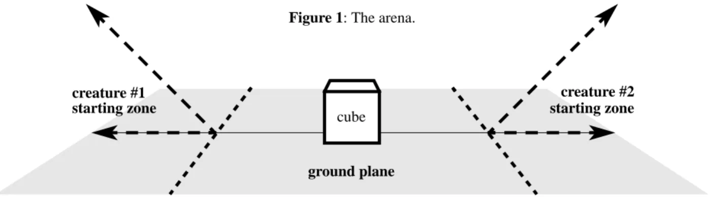
Figure 1 shows the arena in which two virtual creatures will compete to gain control of a single cube. The cube is placed in the center of the world, and the creatures start on opposite sides of the cube. The second contestant is initially turned by 180 degrees so the relative position of the cube to the
crea-ture is consistent from contest to contest no matter which starting side it is assigned. Each creature starts on the ground and behind a diagonal plane slanting up and away from the cube. Creatures are wedged into these “starting zones” until they contact both the ground plane and the diagonal plane, so taller creatures must start further back. This helps prevent the inelegant strategy of simply falling over onto the cube. Strategies like this that utilize only potential energy are fur-ther discouraged by relaxing a creature’s body before it is placed in the starting zone. The effect of gravity is simulated until the creature reaches a stable minimum state.
At the start of the contest the creatures’ nervous sys-tems are activated, and a physical simulation of the crea-tures’ bodies, the cube, and the ground plane begins. The winner is the creature that has the most control over the cube after a certain duration of simulated time (8 seconds were given). Instead of just defining a winner and loser, the mar-gin of victory is determined in the form of a relative fitness value, so there is selection pressure not just to win, but to win by the largest possible margin.
The creatures’ final distances to the cube are used to cal-culate their fitness scores. The shortest distance from any point on the surface of a creatures’s parts to the center of the cube is used as its distance value. A creature gets a higher score by being closer to the cube, but also gets a higher score when its opponent is further away. This encourages creatures to reach the cube, but also gives points for keeping the oppo-nent away from it. If d1 and d2 are the final shortest distances of each creature to the cube, then the fitnesses for each crea-ture, f1 and f2, are given by:
This formulation puts all fitness values in the limited range of 0.0 to 2.0. If the two distances are equal the contestants receive tie scores of 1.0 each, and in all cases the scores will average 1.0. f1 1.0 d2–d1 d1+d2 ---+ = f2 1.0 d1–d2 d1+d2 ---+ = ground plane creature #2 starting zone creature #1 starting zone cube
Credit is also given for having “control” over the cube, beyond just as measured by the minimum distance to it. If both creatures end up contacting the cube, the winner is the one that surrounds it the most. This is approximated by fur-ther decreasing the distance value, as used above, when a creature is touching the cube on the side that opposes its cen-ter of mass. Since the initial distances are measured from the center of the cube they can be adjusted in this way and still remain positive.
During the simulated contest, if neither creature shows any movement for a full second, the simulation is stopped and the scores are evaluated early to save unnecessary com-putation.
3 Approximating Competitive Environments
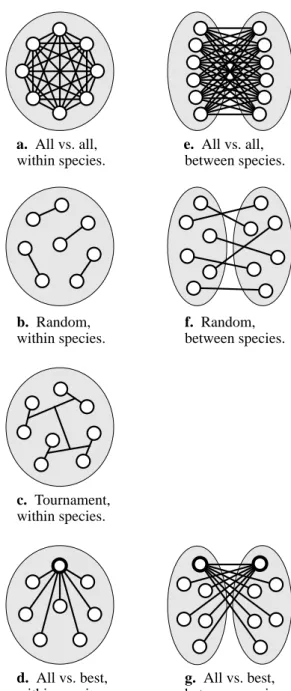
There are many trade-offs to consider when simulating an evolution in which fitness is determined by discrete competi-tions between individuals. In this work, pairs of individuals compete one-on-one. At every generation of a simulated evolution the individuals in the population are paired up by some pattern and a number of competitions are performed to eventually determine a fitness value for every individual. The simulations of the competitions are by far the dominant computational requirement of the process, so the total num-ber of competitions performed for each generation and the effectiveness of the pattern of competitions are important considerations.In one extreme, each individual competes with all the others in the population and the average score determines the fitness (figure 2a). However, this requires (N2 - N)/2 total competitions for a single-species population of N individu-als. For large populations this is often unacceptable, espe-cially if the competition time is significant, as it is in this work.
In the other extreme, each individual competes with just a single opponent (figure 2b). This requires only N/2 total competitions, but can cause inconsistency in the fitness val-ues since each fitness is often highly dependent on the spe-cific individual that happens to be assigned as the opponent. If the pairing is done at random, and especially if the muta-tion rate is high, fitness can be more dependent on the luck of receiving a poor opponent than on an individual’s actual ability.
One compromise between these extremes is for each individual to compete against several opponents chosen at random for each generation. This can somewhat dilute the fitness inconsistency problem, but at the expense of more competition simulations.
A second compromise is a tournament pattern (figure 2c) which can efficiently determine a single overall winner with N - 1 competitions. But this also does not necessarily give all individuals fair scores because of the random initial opponent assignments. Also, this pattern does not easily apply to multi-species evolutions where competitions are not
performed between individuals within the same species. A third compromise is for each individual to compete once per generation, but all against the same opponent. The individual with the highest fitness from the previous genera-tion is chosen as this one-to-beat (figure 2d). This also requires N - 1 competitions per generation, but effectively gives fair relative fitness values since all are playing against the same opponent which has proven to be competent. Vari-ous interesting instabilities can still occur over generations
Figure 2: Different pair-wise competition patterns for one
and two species. The gray areas represent species of inter-breeding individuals, and lines indicate competitions per-formed between individuals.
a. All vs. all, within species. e. All vs. all, between species. b. Random, within species. f. Random, between species. c. Tournament, within species. d. All vs. best, within species. g. All vs. best, between species.
however, since the strategy of the “best” individual can change suddenly between generations.
The number of species in the population is another ele-ment to consider when simulating evolutions involving com-petition. A species may be described as an interbreeding subset of individuals in the population. In single-species evolutions individuals will compete against their relatives, but in multi-species evolutions individuals can optionally compete only against individuals from other species. Figure 2 shows graphical representations of some of the different competition patterns described above for both one and two species.
The resulting effects of using these different competi-tion patterns is unfortunately difficult to quantify in this work, since by its nature a simple overall measure of success is absent. Evolutions were performed using several of the methods described above with both one and two species, and the results were subjectively judged. The most “interesting” results occurred when the all vs. best competition pattern was used. Both one and two species evolutions produced some intriguing strategies, but the multi-species simulations tended to produce more interesting interactions between the evolving creatures. (segment) (leg segment) (body segment) (head)
(body) segment)(limb
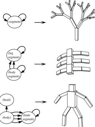
Genotype: directed graph. Phenotype: hierarchy of 3D parts.
Figure 3: Designed examples of genotype graphs and
cor-responding creature morphologies.
4 Creature Morphology
In this work, the phenotype embodiment of a virtual creature is a hierarchy of articulated three-dimensional rigid parts. The genetic representation of this morphology is a directed graph of nodes and connections. Each graph contains the developmental instructions for growing a creature, and pro-vides a way of reusing instructions to make similar or recur-sive components within the creature. A phenotype hierarchy of parts is made from a graph by starting at a defined
root-node and synthesizing parts from the root-node information while
tracing through the connections of the graph. The graph can be recurrent. Nodes can connect to themselves or in cycles to form recursive or fractal like structures. They can also con-nect to the same child multiple times to make duplicate instances of the same appendage.
Each node in the graph contains information describing a rigid part. The dimensions determine the physical shape of the part. A joint-type determines the constraints on the rela-tive motion between this part and its parent by defining the number of degrees of freedom of the joint and the movement allowed for each degree of freedom. The different joint-types allowed are: rigid, revolute, twist, universal,
bend-twist, twist-bend, or spherical. Joint-limits determine the
point beyond which restoring spring forces will be exerted for each degree of freedom. A recursive-limit parameter determines how many times this node should generate a phe-notype part when in a recursive cycle. A set of local neurons is also included in each node, and will be explained further in the next section. Finally, a node contains a set of
connec-tions to other nodes.
Each connection also contains information. The place-ment of a child part relative to its parent is decomposed into
position, orientation, scale, and reflection, so each can be
mutated independently. The position of attachment is con-strained to be on the surface of the parent part. Reflections cause negative scaling, and allow similar but symmetrical sub-trees to be described. A terminal-only flag can cause a connection to be applied only when the recursive limit is reached, and permits tail or hand-like components to occur at the end of chains or repeating units.
Figure 3 shows some simple hand-designed graph topol-ogies and resulting phenotype morpholtopol-ogies. Note that the parameters in the nodes and connections such as
recursive-limit are not shown for the genotype even though they affect
the morphology of the phenotype. The nodes are anthropo-morphically labeled as “body,” “leg segment,” etc. but the genetic descriptions actually have no concept of specific cat-egories of functional components.
5 Creature Behavior
A virtual “brain” determines the behavior of a creature. The brain is a dynamical system that accepts input sensor values and provides output effector values. The output values are applied as forces or torques at the degrees of freedom of the
body’s joints. This cycle of effects is shown in Figure 4. Sensor, effector, and internal neuron signals are repre-sented here by continuously variable scalars that may be pos-itive or negative. Allowing negative values permits the implementation of single effectors that can both push and pull. Although this may not be biologically realistic, it sim-plifies the more natural development of muscle pairs.
5.1 Sensors
Each sensor is contained within a specific part of the body, and measures either aspects of that part or aspects of the world relative to that part. Three different types of sensors were used for these experiments:
1. Joint angle sensors give the current value for each degree of freedom of each joint.
2. Contact sensors activate (1.0) if a contact is made, and negatively activate (-1.0) if not. Each contact sensor has a sensitive region within a part’s shape and activates when any contacts occur in that area. In this work, contact sensors are made available for each face of each part. No distinction is made between self-contact and environmental contact.
3. Photosensors react to a global light source position. Three photosensor signals provide the coordinates of the normalized light source direction relative to the orientation of the part. Shadows are not simulated, so photosensors con-tinue to sense a light source even if it is blocked. Photosen-sors for two independent colors are made available. The source of one color is located in the desirable cube, and the other is located at the center of mass of the opponent. This effectively allows evolving nervous systems to incorporate specific “cube sensors” and “opponent sensors.”
Other types of sensors, such as accelerometers, addi-tional proprioceptors, or even sound or smell detectors could also be implemented, but these basic three are enough to allow some interesting and adaptive behaviors to occur.
5.2 Neurons
Internal neural nodes are used to give virtual creatures the possibility of arbitrary behavior. They allow a creature to have an internal state beyond its sensor values, and be affected by its history.
In this work, different neural nodes can perform diverse functions on their inputs to generate their output signals. Because of this, a creature’s brain might resemble a dataflow computer program more than a typical artificial neural net-work. This approach is probably less biologically realistic than just using sum and threshold functions, but it is hoped that it makes the evolution of interesting behaviors more likely. The set of functions that neural nodes can have is:
sum, product, divide, sum-threshold, greater-than, sign-of, min, max, abs, if, interpolate, sin, cos, atan, log, expt, sig-moid, integrate, differentiate, smooth, memory, oscillate-wave, and oscillate-saw.
Some functions compute an output directly from their
inputs, while others such as the oscillators retain some state and can give time varying outputs even when their inputs are constant. The number of inputs to a neuron depends on its function, and here is at most three. Each input contains a connection to another neuron or a sensor from which to receive a value. Alternatively, an input can simply receive a constant value. The input values are first scaled by weights before being operated on. The genetic parameters for each neural node include these weights as well as the function type and the connection information.
For each simulated time interval, every neuron com-putes its output value from its inputs. In this work, two brain time steps are performed for each dynamic simulation time step so signals can propagate through multiple neurons with less delay.
5.3 Effectors
Each effector simply contains a connection from a neuron or a sensor from which to receive a value. This input value is scaled by a constant weight, and then exerted as a joint force which affects the dynamic simulation and the resulting behavior of the creature. Different types of effectors, such as sound or scent emitters, might also be interesting, but only effectors that exert simulated muscle forces are used here.
Each effector controls a degree of freedom of a joint. The effectors for a given joint connecting two parts, are con-tained in the part further out in the hierarchy, so that each non-root part operates only a single joint connecting it to its parent. The angle sensors for that joint are also contained in this part.
Each effector is given a maximum-strength proportional to the maximum cross sectional area of the two parts it joins. Effector forces are scaled by these strengths and not permit-ted to exceed them. This is similar to the strength limits of natural muscles. As in nature, mass scales with volume but strength scales with area, so behavior does not always scale uniformly.
5.4 Combining Morphology and Control
The genotype descriptions of virtual brains and the actual phenotype brains are both directed graphs of nodes and con-nections. The nodes contain the sensors, neurons, and
effec-Figure 4: Cycle of effects between brain, body and world.
Physical simulation Control system Body 3D World Brain Effectors Sensors
tors, and the connections define the flow of signals between these nodes. These graphs can also be recurrent, and as a result the final control system can have feedback loops and cycles.
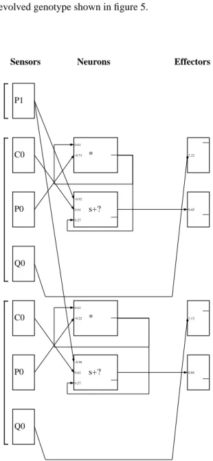
However, most of these neural elements exist within a specific part of the creature. Thus the genotype for the ner-vous system is a nested graph: the morphological nodes each contain graphs of the neural nodes and connections. Figure 5 shows an example of an evolved nested graph which describes a simple three-part creature as shown in figure 6.
When a creature is synthesized from its genetic descrip-tion, the neural components described within each part are generated along with the morphological structure. This causes blocks of neural control circuitry to be replicated along with each instanced part, so each duplicated segment or appendage of a creature can have a similar but indepen-dent local control system.
These local control systems can be connected to enable the possibility of coordinated control. Connections are allowed between adjacent parts in the hierarchy. The neurons and effectors within a part can receive signals from sensors or neurons in their parent part or in their child parts.
Creatures are also allowed a set of neurons that are not associated with a specific part, and are copied only once into the phenotype. This gives the opportunity for the develop-ment of global synchronization or centralized control. These neurons can receive signals from each other or from sensors or neurons in specific instances of any of the creature’s parts, and the neurons and effectors within the parts can optionally receive signals from these unassociated-neuron outputs.
In this way the genetic language for morphology and control is merged. A local control system is described for each type of part, and these are copied and connected into the hierarchy of the creature’s body to make a complete dis-tributed nervous system. Figure 6a shows the creature mor-phology resulting from the genotype in figure 5. Again, parameters describing shapes and weight values are not shown for the genotype even though they affect the
pheno-Figure 5: Example evolved nested graph genotype. The
outer graph in bold describes a creature’s morphology. The inner graph describes its neural circuitry. C0, P0, P1, and Q0 are contact and photosensors, E0 and E1 are effector outputs, and those labeled “*” and “s+?” are neural nodes that perform product and sum-threshold functions.
E0 E1 * s+? P1 C0 P0 Q0 P1 C0 P0 Q0 C0 P0 Q0 * s+? * s+? 2.22 0.65 1.13 0.84 0.61 -0.73 -0.92 0.61 0.27 0.61 -0.22 -0.96 0.61 0.27
Figure 6a: The phenotype morphology generated from
the evolved genotype shown in figure 5.
Figure 6b: The phenotype “brain” generated from the
evolved genotype shown in figure 5. The effector outputs of this control system cause the morphology above to roll forward in tumbling motions.
type. Figure 6b shows the corresponding brain of this crea-ture. The brackets on the left side of figure 6b group the neural components of each part. Two groups have similar neural systems because they were synthesized from the same genetic description. This creature can roll over the ground by making cyclic tumbling motions with its two arm-like appendages. Note that it can be difficult to analyze exactly how a control system such as this works, and some compo-nents may not actually be used at all. Fortunately, a primary benefit of using artificial evolution is that understanding these representations is not necessary.
6 Physical Simulation
Dynamics simulation is used to calculate the movement of creatures resulting from their interaction with a virtual three-dimensional world. There are several components of the physical simulation used in this work: articulated body dynamics, numerical integration, collision detection, and collision response with friction. These are only briefly sum-marized here, since physical simulation is not the emphasis of this paper.
Featherstone’s recursive O(N) articulated body method is used to calculate the accelerations from the velocities and external forces of each hierarchy of connected rigid parts [5]. Integration determines the resulting motions from these accelerations and is performed by a Runge-Kutta-Fehlberg method which is a fourth order Runge-Kutta with an addi-tional evaluation to estimate the error and adapt the step size. Typically between 1 and 5 integration time steps are per-formed for each frame of 1/30 second.
The shapes of parts are represented here by simple rect-angular solids. Bounding box hierarchies are used to reduce the number of collision tests between parts from O(N2). Pairs whose world-space bounding boxes intersect are tested for penetrations, and collisions with a ground plane are also tested. If necessary, the previous time-step is reduced to keep any new penetration depths below a certain tolerance. Con-nected parts are permitted to interpenetrate but not rotate completely through each other. This is achieved by using adjusted shapes when testing for collisions between con-nected parts. The shape of the smaller part is clipped halfway back from its point of attachment so it can swing freely until its remote end makes contact.
Collision response is accomplished by a hybrid model using both impulses and penalty spring forces. At high velocities, instantaneous impulse forces are used, and at low velocities springs are used, to simulate collisions and con-tacts with arbitrary elasticity and friction parameters.
It is important that the physical simulation be reason-ably accurate when optimizing for creatures that can move within it. Any bugs that allow energy leaks from non-conser-vation, or even round-off errors, will inevitably be discov-ered and exploited by the evolving creatures. Although this can be a lazy and often amusing approach for debugging a
physical modeling system, it is not necessarily the most practical.
7 Creature Evolution
An evolution of virtual creatures is begun by first creating an initial population of genotypes. Seed genotypes are synthe-sized “from scratch” by random generation of sets of nodes and connections. Alternatively, an existing genotype from a previous evolution can be used to seed an initial population.
Before creatures are paired off for competitions and fit-ness evaluation, some simple viability checks are performed, and inappropriate creatures are removed from the population by giving them zero fitness values. Those that have more than a specified number of parts are removed. A subset of genotypes will generate creatures whose parts initially inter-penetrate. A short simulation with collision detection and response attempts to repel any intersecting parts, but those creatures with persistent interpenetrations are also discarded. A survival-ratio determines the percentage of the popu-lation that will survive each generation. In this work, popula-tion sizes were typically 300, and the survival-ratio was 1/5. If the initially generated population has fewer individuals with positive fitness than the number that should survive, another round of seed genotypes is generated to replace those with zero fitness.
For each generation, creatures are grown from their gen-otypes, and their fitness values are measured by simulating one or more competitions with other individuals as described. The individuals whose fitnesses fall within the survival percentile are then reproduced, and their offspring fill the slots of those individuals that did not survive. The number of offspring that each surviving individual generates is proportional to its fitness. The survivors are kept in the population for the next generation, and the total size of the population is maintained. In multi-species evolutions, each sub-population is independently treated in this way so the number of individuals in each species remains constant and species do not die out.
Offspring are generated from the surviving creatures by copying and combining their directed graph genotypes. When these graphs are reproduced they are subjected to probabilistic variation or mutation, so the corresponding phenotypes are similar to their parents but have been altered or adjusted in random ways.
7.1 Mutating Directed Graphs
A directed graph is mutated by the following sequence of steps:
1. The internal parameters of each node are subjected to possible alterations. A mutation frequency for each parame-ter type deparame-termines the probability that a mutation will be applied to it at all. Boolean values are mutated by simply flipping their state. Scalar values are mutated by adding sev-eral random numbers to them for a Gaussian-like distribution
so small adjustments are more likely than drastic ones. The scale of an adjustment is relative to the original value, so large quantities can be varied more easily and small ones can be carefully tuned. A scalar can also be negated. After a mutation occurs, values are clamped to their legal bounds. Some parameters that only have a limited number of legal values are mutated by simply picking a new value at random from the set of possibilities.
2. A new random node is added to the graph. A new node normally has no effect on the phenotype unless a con-nection also mutates a pointer to it. Therefore a new node is always initially added, but then garbage collected later (in step 5) if it does not become connected. This type of muta-tion allows the complexity of the graph to grow as an evolu-tion proceeds.
3. The parameters of each connection are subjected to possible mutations in the same way the node parameters were in step 1. With some frequency the connection pointer is moved to point to a different node which is chosen at ran-dom.
4. New random connections may be added and existing ones may be removed. In the case of the neural graphs these operations are not performed because the number of inputs for each element is fixed, but the morphological graphs can have a variable number of connections per node. Each exist-ing node is subject to havexist-ing a new random connection added to it, and each existing connection is subject to possi-ble removal.
5. Unconnected elements are garbage collected. Con-nectedness is propagated outwards through the connections of the graph, starting from the root node of the morphology, and from the effector nodes of the neural graphs. Although leaving the disconnected nodes for possible reconnection might be advantageous, and is probably biologically analo-gous, at least the unconnected newly added ones are removed to prevent unnecessary growth in graph size.
Since mutations are performed on a per element basis, genotypes with only a few elements might not receive any mutations, where genotypes with many elements would receive enough mutations that they would rarely resemble their parents. This is compensated for by scaling the muta-tion frequencies by an amount inversely propormuta-tional to the size of the current graph being mutated, such that on the average at least one mutation occurs in the entire graph.
Mutation of nested directed graphs, as are used here to represent creatures, is performed by first mutating the outer graph and then mutating the inner layer of graphs. The inner graphs are mutated last because legal values for some of their parameters (inter-node neural input sources) can depend on the topology of the outer graph.
7.2 Mating Directed Graphs
Sexual reproduction allows components from more than one parent to be combined into new offspring. This permits fea-tures to evolve independently and later be merged into a
sin-gle individual. Two different methods for mating directed graphs are used in this work.
The first is a crossover operation (figure 7a). The nodes of two parents are each aligned in a row as they are stored, and the nodes of the first parent are copied to make the child, but one or more crossover points determine when the copy-ing source should switch to the other parent. The connec-tions of a node are copied with it and simply point to the same relative node locations as before. If the copied connec-tions now point out of bounds because of varying node num-bers they are randomly reassigned.
A second mating method grafts two genotypes together by connecting a node of one parent to a node of another (fig-ure 7b). The first parent is copied, and one of its connections is chosen at random and adjusted to point to a random node in the second parent. Newly unconnected nodes of the first parent are removed and the newly connected node of the sec-ond parent and any of its descendants are appended to the new graph.
A new directed graph can be produced by either of these two mating methods, or asexually by using only mutations. Offspring from matings are sometimes subjected to muta-tions afterwards, but with reduced mutation frequencies. In this work a reproduction method is chosen at random for each child to be produced by the surviving individuals using the ratios: 40% asexual, 30% crossovers, and 30% grafting. A second parent is chosen from the survivors if necessary, and a new genotype is produced from the parent or parents.
After a new generation of genotypes is created, a pheno-type creature is generated from each, and again their fitness values are evaluated. As this cycle of variation and selection continues, the population is directed towards creatures with higher fitness.
7.3 Parallel Implementation
This process has been implemented to run in parallel on a Connection Machine® CM-5 in a master/slave message
pass-ing model. A spass-ingle processpass-ing node contains the population and performs all the selection and reproduction operations. It farms out pairs of genotypes to the other nodes to be fitness tested, and gathers back the fitness values after they have been determined. The fitness tests each include a dynamics
Figure 7: Two methods for mating directed graphs.
a. Crossovers: b. Grafting: parent 1 parent 2 child parent 1 parent 2 child
simulation for the competition and although many can exe-cute in nearly real-time, they are still the dominant computa-tional requirement of the system. Performing a fitness test per processor is a simple but effective way to parallelize this process, and the overall performance scales quite linearly with the number of processors, as long as the population size is somewhat larger than the number of processors.
Each fitness test takes a different amount of time to compute depending on the complexity of the creatures and how they attempt to move. To prevent idle processors from just waiting for others to finish, the slowest few simulations at the end of a generation are suspended and those individu-als are removed from the population by giving them zero fit-ness. With this approach, an evolution with population size 300, run for 100 generations, might take about four hours to complete on a 32 processor CM-5.
8 Results and Discussion
Many independent evolutions were performed using the “all vs. best” competition pattern as described in section 3. Some single-species evolutions were performed in which all indi-viduals both compete and breed with each other, but most included two species where individuals only compete with members of the opponent species.
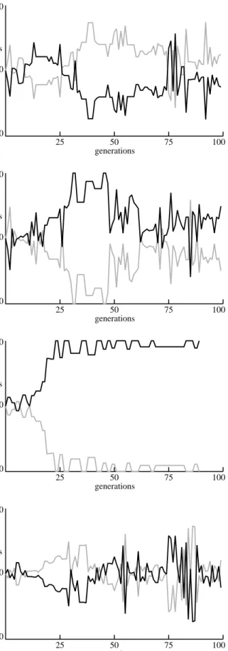
Some examples of resulting two-species evolutionary dynamics are shown in Figure 8. The relative fitness of the best individuals of each species are plotted over 100 genera-tions. The rate of evolutionary progress varied widely in dif-ferent runs. Some species took many generations before they could even reach the cube at all, while others discovered a fairly successful strategy in the first 10 or 20 generations. Figure 8c shows an example where one species was success-ful fairly quickly and the other species never evolved an effective strategy to challenge it. The other three graphs in figure 8 show evolutions where more interactions occurred between the evolving species.
A variety of methods for reaching the cube were discov-ered. Some extended arms out onto the cube, and some reached out while falling forward to land on top of it. Others could crawl inch-worm style or roll towards the cube, and a few even developed leg-like appendages that they used to walk towards it.
The most interesting results often occurred when both species discovered methods for reaching the cube and then further evolved strategies to counter the opponent’s behav-ior. Some creatures pushed their opponent away from the cube, some moved the cube away from its initial location and then followed it, and others simply covered up the cube to block the opponent’s access. Some counter-strategies took advantage of a specific weakness in the original strategy and could be easily foiled in a few generations by a minor adap-tation to the original strategy. Others permanently defeated the original strategy and required the first species to evolve another level of counter-counter-strategy to regain the lead.
Figure 8: Relative fitness between two co-evolving and
competing species, from four independent simulations.
a.
generations fitness 0.0 1.0 2.0 25 50 75 100b.
generations fitness 0.0 1.0 2.0 25 50 75 100c.
generations fitness 0.0 1.0 2.0 25 50 75 100d.
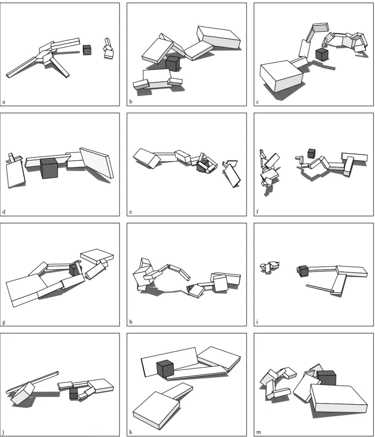
generations fitness 0.0 1.0 2.0 25 50 75 100Figure 9: Evolved competing creatures.
a b c
d e f
g h i
In some evolutions the winners alternated between species many times with new strategies and counter-strategies. In other runs one species kept a consistent lead with the other species only providing temporary challenges.
After the results from many simulations were observed, the best were collected and then played against each other in additional competitions. The different strategies were com-pared, and the behavior and adaptability of creatures were observed as they faced new types of opponents that were not encountered during their evolutions. A few evolutions were also performed starting with an existing creature as a seed genotype for each species so they could further evolve to compete against a new type of opponent.
Figure 9 shows some examples of evolved competing creatures and demonstrates the diversity of the different strategies that emerged. Some of the behaviors and interac-tions of these specific creatures are described briefly here. The larger creature in figure 9b nudges the cube aside and then pins down his smaller opponent. The crab-like creature in 9c can successfully walk forward, but then continues blindly past the cube and over the opponent. Figure 9d shows a creature that has just pushed its opponent away from the cube, and the arm-like creature in 9e also jabs at its oppo-nent before curling around the cube.
Most creatures perform similar behavior independently of the opponent’s actions, but a few are adaptive in that they can reach towards the cube wherever it moves. For example the arm-like creature in figure 9f pushes the cube aside and then uses photosensors to adaptively follow it. If its oppo-nent moves the cube in a different direction it will success-fully grope towards the new location.
The two-armed creature in figure 9g blocks access to the cube by covering it up. Several other two-armed creatures in 9i, 9j, and 9k use the strategy of batting the cube to the side with one arm and catching it with the other arm. This seemed to be the most successful strategy of the creatures in this group, and the one in 9k was actually the overall winner because it could whisk the cube aside very quickly. How-ever, it was a near tie between this and the photosensitive arm in 9f. The larger creature in 9m wins by a large margin against some opponents because it can literally walk away with the cube, but it does not initially reach the cube very quickly and tends to loose against faster opponents.
It is possible that adaptation on an evolutionary scale occurred more easily than the evolution of individuals that were themselves adaptive. Perhaps individuals with adaptive behavior would be significantly more rewarded if evolutions were performed with many species instead of just one or two. To be successful, a single individual would then need to defeat a larger number of different opposing strategies.
9 Future Work
Several variations on this system could be worth further experimentation. Other types of contests could be defined in
which creatures compete in different environments and dif-ferent rules determine the winners. Creatures might also be rewarded for cooperative behavior somehow as well as com-petitive, and teams of interacting creatures could be simu-lated.
Evolutions containing larger numbers of species should certainly be performed, with the hope of increasing the chances for emergence of more adaptive individuals as hypothesized above.
An additional extension to this work would be to simu-late a more complex but more realistic environment in which many creatures simultaneously compete and/or cooperate with each another, instead of pairing off in one-on-one con-tests. Speciation, mating patterns, competing patterns, and even offspring production could all be determined by one long ecological simulation. Experiments like this have been performed with simpler organisms and have produced inter-esting results including specialization and various social interactions [18,24].
Perhaps the techniques presented here should be consid-ered as an approach toward creating artificial intelligence. When a genetic language allows virtual entities to evolve with increasing complexity, it is common for the resulting system to be difficult to understand in detail. In many cases it would also be difficult to design a similar system using tradi-tional methods. Techniques such as these have the potential of surpassing those limits that are often imposed when human understanding and design is required. The examples presented here suggest that it might be easier to evolve vir-tual entities exhibiting intelligent behavior than it would be for humans to design and build them.
10 Conclusion
In summary, a system has been described that can automati-cally generate autonomous three-dimensional virtual crea-tures that exhibit diverse competitive strategies in physically simulated worlds. A genetic language that uses directed graphs to describe both morphology and behavior defines an unlimited hyperspace of possible results, and a variety of interesting virtual creatures have been shown to emerge when this hyperspace is explored by populations of evolving and competing individuals.
Acknowledgments
Thanks to Gary Oberbrunner and Matt Fitzgibbon for Con-nection Machine and software support. Thanks to Thinking Machines Corporation and Lew Tucker for supporting this research. Thanks to Bruce Blumberg and Peter Schröder for dynamic simulation help and suggestions. And special thanks to Pattie Maes.
References
1. Angeline, P.J., and Pollack, J.B., “Competitive Environ-ments Evolve Better Solutions for Complex Tasks,” in
Proceedings of the 5th International Conference on Genetic Algorithms, ed. by S. Forrest, Morgan
Kauf-mann 1993, pp.264-270.
2. Axelrod, R., “Evolution of Strategies in the Iterated Prisoner’s Dilemma”, in Genetic Algorithms and
Simu-lated Annealing, ed. by L. Davis, Morgan Kaufmann,
1989.
3. Cramer, N.L., “A Representation for the Adaptive Gen-eration of Simple Sequential Programs,” Proceedings of
the First International Conference on Genetic Algo-rithms, ed. by J. Grefenstette, 1985, pp.183-187.
4. Dawkins, R., The Blind Watchmaker, Harlow Longman, 1986.
5. Featherstone, R., Robot Dynamics Algorithms, Kluwer Academic Publishers, Norwell, MA, 1987.
6. de Garis, H., “Genetic Programming: Building Artificial Nervous Systems Using Genetically Programmed Neu-ral Network Modules,” Proceedings of the 7th
Interna-tional Conference on Machine Learning, 1990,
pp.132-139.
7. Goldberg, D.E., Genetic Algorithms in Search,
Optimi-zation, and Machine Learning, Addison-Wesley, 1989.
8. Hart, J., “The Object Instancing Paradigm for Linear Fractal Modeling,” Graphics Interface, 1992, pp.224-231.
9. Hillis, W.D., “Co-evolving parasites improve simulated evolution as an optimization procedure,” Artificial Life
II, ed. by Langton, Taylor, Farmer, & Rasmussen,
Addi-son-Wesley, 1991, pp313-324.
10. Holland, J.H., Adaptation in Natural and Artificial
Sys-tems, Ann Arbor, University of Michigan Press, 1975.
11. Kitano, H., “Designing neural networks using genetic algorithms with graph generation system,” Complex
Systems, Vol.4, pp.461-476, 1990.
12. Koza, J., Genetic Programming: on the Programming of
Computers by Means of Natural Selection, MIT Press,
1992.
13. Lindenmayer, A., “Mathematical Models for Cellular Interactions in Development, Parts I and II,” Journal of
Theoretical Biology, Vol.18, 1968, pp.280-315.
14. Lindgren, K., “Evolutionary Phenomena in Simple Dynamics,” in Artificial Life II, ed. by Langton, Taylor, Farmer, & Rasmussen, Addison-Wesley, 1991, pp.295-312.
15. Mjolsness, E., Sharp, D., and Alpert, B., “Scaling, Machine Learning, and Genetic Neural Nets,” Advances
in Applied Mathematics, Vol.10, 1989, pp.137-163.
16. Ngo, J.T., and Marks, J., “Spacetime Constraints Revis-ited,” Computer Graphics, Annual Conference Series, 1993, pp.343-350.
17. van de Panne, M., and Fiume, E., “Sensor-Actuator Net-works,” Computer Graphics, Annual Conference Series, 1993, pp.335-342.
18. Ray, T., “An Approach to the Synthesis of Life,”
Artifi-cial Life II, ed. by Langton, Taylor, Farmer, &
Rasmus-sen, Addison-Wesley, 1991, pp.371-408.
19. Reynolds, C., “Competition, Coevolution and the Game of Tag,” to be published in: Artificial Life IV
Proceed-ings, ed. by R. Brooks & P. Maes, MIT Press, 1994.
20. Sims, K., “Artificial Evolution for Computer Graphics,”
Computer Graphics, Vol.25, No.4, July 1991,
pp.319-328.
21. Sims, K., “Interactive Evolution of Dynamical Sys-tems,” Toward a Practice of Autonomous Systems:
Pro-ceedings of the First European Conference on Artificial Life, ed. by Varela, Francisco, & Bourgine, MIT Press,
1992, pp.171-178.
22. Sims, K., “Evolving Virtual Creatures,” Computer
Graphics, Annual Conference Series, July 1994,
pp.15-22.
23. Smith, A.R., “Plants, Fractals, and Formal Languages,”
Computer Graphics, Vol.18, No.3, July 1984, pp.1-10.
24. Yaeger, L., “Computational Genetics, Physiology, Metabolism, Neural Systems, Learning, Vision, and Behavior or PolyWorld: Life in a New Context,”
Artifi-cial Life III, ed. by C. Langton, Santa Fe Institute
Stud-ies in the Sciences of Complexity, Proceedings Vol. XVII, Addison-Wesley, 1994, pp.263-298.