Libor and Swap Market Models for the Pricing of Interest Rate Derivatives: An Empirical Analysis

Center for

Economic Research

No. 2000-35

LIBOR AND SWAP MARKET MODELS FOR THE PRICING OF INTEREST RATE DERIVATIVES: AN EMPIRICAL ANALYSIS

By Frank de Jong, Joost Driessen and Antoon Pelsser

March 2000

Libor and Swap Market Models

for the Pricing of Interest Rate Derivatives:

An Empirical Analysis

Frank De Jong

Joost Driessen

Antoon Pelsser

First version: February 23, 1999

This version: February 24, 2000

We thank B.A. Jensen, Bas Werker, participants of the Eurandom Workshop Eindhoven 1999, the QMF-99 Conference in Sydney and the EFA-99 Conference in Helsinki, as well as seminar participants at Hebrew University, University of Leuven, Tilburg University, and the National Research Institute for Mathematics and Computer Science, for their helpful comments.

Frank de Jong, Finance Group, University of Amsterdam, Roetersstraat 11, 1018 WB, Amsterdam, The Netherlands. Tel: +31-20-5255815. E-mail: fdejong@fee.uva.nl.

Joost Driessen, Department of Econometrics, Tilburg University, PO Box 90153, 5000 LE, Tilburg, The Netherlands. Tel: +31-13-4663219. E-mail: jdriesse@kub.nl.

Antoon Pelsser, ABN-AMRO Bank, Structured Products Group (AA4410), PO Box 283, 1000 EA Amsterdam, The Netherlands. Tel: +31-20-6286538. E-mail: antoon.pelsser@nl.abnamro.com.

Libor and Swap Market Models

for the Pricing of Interest Rate Derivatives:

An Empirical Analysis

Abstract

In this paper we empirically analyze and compare the Libor and Swap Market Models, developed by Brace, Gatarek, and Musiela (1997) and Jamshidian (1997), using paneldata on prices of US caplets and swaptions. A Libor Market Model can directly be calibrated to observed prices of caplets, whereas a Swap Market Model is calibrated to a certain set of swaption prices. For both one-factor and two-factor models we analyze how well they price caplets and swaptions that were not used for calibration. We show that the Libor Market Models in general lead to better prediction of derivative prices that were not used for calibration than the Swap Market Models. A one-factor Libor Market Model that exhibits mean-reversion gives a good fit of the derivative prices, and adding a second factor only decreases pricing errors to a small extent. We also find that models that are chosen to exactly match certain derivative prices are overfitted. Finally, a regression analysis reveals that the pricing errors are correlated with the shape of the term structure of interest rates.

JEL Codes: G12, G13, E43.

1

Recent work on the market models includes Andersen and Andreasen (1998), Barton, Brace, and Dun (1998), Glasserman and Zhao (1998), Longstaff, Santa-Clara, and Schwartz (1999), Pedersen (1999), Rebonato (1999), and Schlögl (1999).

1 Introduction

Since the first interest rate swap was traded in 1981, the market for interest rate derivatives has grown enormously. Both the volume and complexity of the products traded has increased. Hence, the modelling and pricing of interest rate derivatives has been an area of research of considerable interest both for academics and practitioners.

To determine the prices of exotic interest rate derivatives, pricing models are used as an 'extrapolation tool'. Given the prices of liquid instruments available in the market, such as caps and swaptions, pricing models extract information about the distribution of the underlying rates by calibrating to these market prices. The calibrated model is then used to price and hedge the exotic instrument. For the successful pricing of exotic options, it is therefore important to find parsimoniously specified models that provide an accurate fit to the prices of the liquid market derivative instruments.

A recent development in modelling interest rates and pricing interest rate derivatives are the so-called market models. Brace, Gatarek, and Musiela (1997) and Miltersen, Sandmann, and Sondermann (1997) present an arbitrage-free interest rate model, the Libor Market Model (LMM), in which forward Libor rates follow lognormal processes, leading to the Black (1976) pricing formula for caps and floors, which is used by market practitioners. A similar model for swap rates and swap rate derivatives was developed by Jamshidian (1997). His so-called Swap Market Model (SMM) leads to the Black formula for swaptions. There are several advantages of the market models in comparison with the traditional models, such as the instantaneous spot rate models (e.g. Vasicek (1977), Hull and White (1990), and Cox, Ingersoll and Ross (1985)) and models for instantaneous forward interest rates (Heath, Jarrow and Morton (1992) and Ritchken and Sankarasubramanian (1995)). First, the match to the market Black formula for option prices makes calibration of market models very simple, since the quoted implied Black volatilities can directly be inserted in the model, avoiding the numerical fitting procedures that are needed for the spot rate or forward rate models. Second, the market models are based on observable market rates, such as Libor rates and swap rates. Hence, one does not need the (unobserved) instantaneous short rate or instantaneous forward rates to price and hedge caps and swaptions.

Given the advantages of the market models, it is not surprising these models have received a lot of attention recently1_{. There has been little attention however to the empirical performance of the market}

models. Since the LMM and the SMM are mutually inconsistent approaches, it is an empirical question which model is to be preferred for practical purposes. In this paper we therefore empirically analyze the Libor and Swap Market Models. We use panel data on prices of caplets of different option maturities, and prices of the swaption ‘matrix’ (i.e. prices of swaptions for several option maturities and swap maturities).

The paper focuses on four important issues.

The first is an empirical comparison of the LMM with the SMM. Our empirical approach is to calibrate the LMM on a set of caplet prices, and subsequently calculate the prices for swaptions implied by the LMM. Similarly, we calibrate the SMM to a subset of swaption prices, namely all swaptions for which the total maturity, defined as the sum of the option and swap maturity, is equal to 10 years, and subsequently calculate the prices implied by the SMM for swaptions with total maturities less than 10 years and caplets. To compare the LMM with the SMM, we use the differences between model prices and actual prices for the swaptions with a total maturity less than 10 years, which are the instruments that are not used for calibration of the LMM and the SMM. The empirical results show that the LMM in general leads to better prediction of these swaption prices than the SMM. Also, the SMM substantially overprices caplets. In this paper, we provide an explanation for these results.

A second important issue in calibrating the model is the specification of the volatility function. This function plays a crucial role in the model. We show that the usual choice of a constant volatility function for each option maturity date is not a particularly good one, because the LMM with a constant volatility function persistently overprices swaptions and the SMM with a constant volatility function underprices swaptions. Much better results are obtained by specifying an exponentially increasing volatility function. This functional form endows the model with mean-reverting behaviour of interest rates and decreases the correlation between interest rates at different dates.

The third issue we examine is the empirically relevant number of factors. In a recent paper, Longstaff, Santa-Clara, and Schwartz (1999) argue that for the pricing of American swaptions, a large number of factors is required in a constant volatility SMM-like model. In contrast, we show that a (carefully calibrated) one factor model with an exponential volatility function (mean reversion) suffices for the pricing of European caplets and swaptions. The pricing errors for two-factor models are only a little smaller than the pricing errors for the one-factor models, which implies that the one-factor assumption is not very restrictive for this particular application.

Fourth, we consider two different calibration methodologies: exact calibration and non-exact calibration. In case of exact calibration, the model under consideration has as many parameters as calibration instruments, and these parameters are chosen such that the model exactly fits caplets (in case of the LMM) or 10-year total maturity swaptions (in case of the SMM). With non-exact calibration, the model has only a small number of parameters, and exact fitting of derivative prices is not possible in general. This setup allows us to examine whether exact calibration leads to overfitting, in the sense that some parameters are to a large extent fitted to noise in the derivative price quotes. We indeed find that the exactly calibrated models overfit the derivative price data, as in almost all cases non-exact calibration leads to smaller pricing errors for the options that are not used for calibration than exact calibration.

For all models and calibration methodologies, a specification test reveals that the market models are rejected statistically, but given the large bid-ask spreads on these derivative instruments, the size of the pricing errors does not seem to be economically very large. Still, the pricing errors of all one-factor models

are correlated with variables that are associated with the shape of the term structure, i.e. level, steepness and curvature variables. This could be the result of the one-factor assumption. However, the pricing errors of the two-factor models are also correlated with the shape of the term structure. We argue that the misspecification is more likely to be the result of the assumption of lognormally distributed interest rates. This paper is related to previous empirical work on pricing interest rate derivatives. Flesaker (1993) and Amin and Morton (1994) analyze the pricing of Eurodollar futures options with Heath, Jarrow, and Morton (HJM, 1992) models. In both articles only one-factor models are examined. The effect of mean-reversion on the pricing of derivative prices is analyzed by Amin and Morton (1994), but since they only use short-maturity options on short-short-maturity futures, they are not able to precisely estimate the effect of mean-reversion. As our dataset contains a wide range of option and swap maturities, we are able to precisely estimate the strength of the mean-reversion as well as the effect of mean-reversion on the pricing of swaptions. Amin and Morton (1994) also examine whether models are overfitted to derivative prices by analyzing whether model-based trading strategies are profitable. They conclude that models with only two calibration parameters are overfitted to the derivative prices. In this paper, we provide a more direct analysis of model overfitting, by studying the prediction of derivative prices that are not used for calibration. Buhler et al. (1999) use data on German government bond options to compare several one- and two-factor interest rate models. Buhler et al. (1999) estimate the model parameters from historical interest rate data, which leads to very large pricing errors for the bond options. Such an estimation procedure can be useful for the calculation of risk measures, such as VaR. For the accurate pricing of exotic interest rate derivatives however, it seems inevitable to also use the information in derivative prices to estimate the model parameters. In general, our study differs from the current literature because we analyze the new class of market models, and because we use both caplets and swaptions for our analysis.

The remainder of this paper is organized as follows. In section 2, we briefly review the construction of the market models. Section 3 describes the data. Section 4 first discusses the calibration methodology for the LMM and then presents the results of this calibration. Section 5 presents the calibration methodology and results for the SMM. In section 6 we analyze two-factor Libor Market Models. In section 7 we summarize and conclude.

2

In Brace, Gatarek, and Musiela (1997), a formulation based on a continuum of bond prices is presented, so that the LMM fits in the framework of Heath, Jarrow, and Morton (1992). However, as noted by Jamshidian (1997), for the pricing and hedging of caplets and swaptions it is not necessary that a continuum of bond prices and a money market account exist. This is an important difference between the market models and the framework of Heath, Jarrow, and Morton (1992).

3

Because of daycount conventions the daycount fractions are actually functions*i = g(Ti,, Ti-1), that are only

approximately equal to (Ti - Ti-1

)

.

T₁ < T₂ < ... < T_N

(1)

(2)

2 Libor and Swap Market Models

In this section we describe the market models of interest rates. We first show how a Libor Market Model (LMM) is constructed. Thereafter, we briefly discuss the formulation of a Swap Market Model (SMM). For a complete discussion of the Swap Market Models, we refer to Jamshidian (1997) and Musiela and Rutkowski (1998). For both models, we briefly discuss the pricing of caplets and swaptions.

2.1 The Libor Market Model

We describe the LMM formulation based on a finite number of bond prices, following Jamshidian (1997).2

We start with defining a finite set of dates, the so-called tenor structure,

We also define *_i ' _T as the so-called daycount fractions, which are determined by the

i%₁&T_i, i'1,..,N&1

maturity of the Libor rate that is used to determine caplet payoffs and are most often equal to 3 or 6 months3. Associated with each tenor date Tn is a bond that matures at this date, and its time t price is denoted with P_n(t). It is assumed that these bond prices follow Itô processes under the empirical probability measure, i.e.

where Wt is a standard Brownian Motion, and in this paper it is assumed to be one- or two-dimensional. The one-dimensional drift function µP_n(t) and the bond price volatility FP_n(t), that has the same dimension as Wt, can depend on the bond price P_n(t). The forward Libor rate at time t for the accrual period [T_n,T_n%₁]

4

The no-arbitrage condition used here is weaker than the usual no-arbitrage condition, because the existence of a continuous savings account is not assumed here, see Jamshidian (1997) for details. In the continuous-tenor case of Brace, Gatarek and Musiela (1997), the usual no-arbitrage condition is used.

L_n(t) ' 1 *_n ( P_n(t) P_n%1(t) &_{1), n}'_1,...,N&₁

(3)

(4)

Applying Itô’s division rule to equation (3), it follows that a forward Libor rate satisfies the following Itô process under the empirical probability measure

The function µ_n(t) is the drift function of the forward Libor rate, and (_n(t) is the volatility function. The idea behind the LMM is to construct an arbitrage-free interest rate model that implies a pricing formula for caplets that has the same structure as the Black pricing formula for a caplet, that is used by market practitioners. As the Black pricing formula for a caplet is based on the assumption that the relevant forward Libor rate follows a lognormal process under the equivalent martingale measure, the LMM has to imply lognormal processes (under the equivalent martingale measure) for the forward Libor rates in (3). It is therefore assumed that the volatility function (_n(t) is a deterministic function of time, which can be different for the different forward Libor rates. For a given forward Libor rate, this volatility function describes the instantaneous volatility of this forward Libor rate over time, until the forward

(_n(t), t#T_n,

Libor rate matures at time T_n. If this volatility function is constant, i.e. if (_n(t) does not depend on t, the volatility of the forward Libor rate L_n(t) is constant until its maturity date T_n. A volatility function (_n(t) that is increasing in time t would imply that the volatility of the forward Libor rate increases as the rate approaches its maturity date. Such a volatility function would be consistent with mean-reverting behaviour of interest rates, as mean-reversion typically implies that interest rates close to maturity have a larger volatility than interest rates that are far from maturity.

Given these N-1 volatility functions of the forward Libor rates, the N volatility functions of the bond prices cannot be recovered. This indeterminacy is solved by choosing one of these bond prices as numeraire. By assuming that there are no arbitrage opportunities4 _{amongst the N bonds, it follows (see}

dL_n(t) ' _L n(t) (& j N&₁ i'_n%₁ *_iL_i(t)(_i(t)y(_n(t) 1%_* iLi(t) dt % ( n(t) y_dW( t ), n'1,...,N&1

(5)

(6)

(7)

martingales in the probability measure associated with the choice of the numeraire. One convenient choice for the numeraire asset is the bond with the longest maturity P_N(t), and the associated probability measure is often called the terminal measureQN_{. Jamshidian (1997) shows that the process of forward Libor rates} under the terminal measure is given by

where _W( is a standard Brownian Motion under the terminal measure. Given the QN_{-processes of these} t

N-1 forward Libor rates, all numeraire-denominated bond price processes can be determined.

The result in (5) implies that, in order to price and hedge interest rate derivatives, only the volatility functions (_n(t) have to be determined. Furthermore, under the terminal measure, the Libor rateL_N&1(t) has zero drift. Similarly, under the probability measure Qn _{associated with the numeraire P , the Libor rate}

n(t) Ln&₁(t)

has zero drift. This directly follows from the fact that the Libor rate L_n&1(t) is a ratio of bond prices, with the numeraire P_n(t) in the denominator, as shown in equation (3).

We now turn to the pricing of (European) interest rate derivatives, such as caplets, caps and swaptions. A caplet with strike rate k and maturity date Tn pays off *n(Ln(Tn)&k) at time Tn+1. The LMM-price of

%

this caplet at time t can be calculated using the expectation of the discounted payoff under the Qn+1 _measure

and because _L follows a driftless lognormal process under the Qn+1 _{measure, equation (6) leads to the} n(t)

familiar Black pricing formula for a caplet and this caplet price is determined by the conditional variance (under the Qn+1_{-measure) of the forward Libor rate over the maturity of the caplet, which is equal to} . The price of a cap, which is a sum of caplets of different maturities, can therefore also

m

Tn

t

(_n(s)y(_n(s)ds

analytically be determined for the LMM.

A swaption is an option on a swap. Consider a forward swap, with principal 1, where two parties agree to exchange at dates {T_n%₁,...,T_n%_m} the floating Libor rates {L_n(t),...,L_n%_m&₁(t)} for a fixed rate. The forward swap rate is the fixed rate that gives this contract zero initial value and is given by

dS_n,N&_n(t) ' S_n,N&_n(t) ( µ_n,N&_n(t)dt % (_n,N&_n(t)ydW_t), n'1,...,N&1

(8)

A payers swaption with strike rate k, maturity date Tn and m payment dates gives right to enter into a swap at date Tn, where floating Libor payments are received and fixed payments k are paid. Equivalently, a payers swaption gives the right to receive the cash flow *_n%_j&₁(S_n,m(T_n)&k) at dates (see

%

T_n%_j, j'1,..,m

Musiela and Rutkowski (1997)).

In equation (7), it is shown that a forward swap rate depends on several forward Libor rates, so that the variance of a swap rate is a function of both the variances and covariances (or correlations) of forward Libor rates. Swaption prices thus depend both on conditional variances and covariances of forward Libor rates of different maturities, whereas caplet prices only depend on the conditional variance of one forward Libor rate. It is easy to show that forward swap rates do not follow lognormal processes in the LMM, as the forward par swap rate in (7) is a linear combination of several forward Libor rates. Swaptions can not be priced analytically by the LMM. We will use simulation to obtain (exact) prices of swaptions, by simulating the Euler discretization of the processes of forward Libor rates in equation (5) under the terminal measure. The complete simulation procedure is described in Brace (1998).

2.2 The Swap Market Model

The SMM is constructed in a way that is quite similar to the construction of the LMM, but the algebra is more complicated. Therefore we will only briefly discuss the construction of the SMM, and again refer to Jamshidian (1997) for a detailed discussion. The SMM is also used by Longstaff, Santa-Clara, and Schwartz (1999) in an analysis of the pricing of American swaptions.

We start with the same tenor structure as given in equation (1), and we again assume that the N bond prices follow Itô processes. To arrive at the Black-type pricing formula for swaptions, we will now require that forward swap rates follow lognormal processes. More specifically, for the set of forward swap rates that have the same enddate TN, Sn,N&n(t), n'1,...,N, it is assumed that under the empirical probability

measure

Given the N-1 deterministic volatility functions (_n,N&n(t) of the forward swap rates, the N volatility functions of bond prices cannot be determined and again this indeterminacy is resolved by choosing a bond price as numeraire. For the forward swap rate S_n,N&n(t) the most convenient choice of numeraire is the

coupon process or present value of a basis point (PVBP) _jN_j'&₁n *_n%j&1Pn%j(t). Equation (7) shows that, assuming no-arbitrage and choosing this coupon process as numeraire, the forward swap rate S_n,N&n(t)

follows a driftless lognormal process under the equivalent martingale measure induced by this numeraire choice. This directly implies that the SMM-price of a swaption with option maturity T_n and swap maturity T_N&_T

n

5

The data are provided by ABN-AMRO Bank. The implied volatilities for caplets are obtained from data on cap implied volatilities, using bootstrap methods described in Hull (1997).

maturity plus the swap maturity, equal to TN will have a Black-type pricing formula, as the forward swap rates that determine these swaption prices follow driftless lognormal processes under their equivalent martingale measures. Again, determination of the volatilities (_n,N&_n(t) is all that is necessary to price derivatives.

The prices of other swaptions and caplets cannot be determined using the closed-form Black formula, as the underlying rates do not follow lognormal processes in the SMM, and we use simulation techniques to obtain prices. Of course, we simulate all forward swap rates under the same equivalent martingale measure, induced by a particular numeraire choice. We choose to simulate under the terminal equivalent martingale measure, using an Euler discretization of the processes of forward swap rates under this measure, which are derived by Jamshidian (1997).

The difference between the LMM and the SMM is therefore determined by the set of market rates that follow lognormal processes in the model. For the LMM this is a set of forward Libor rates, and for the SMM this is a set of forward swap rates.

3 Data Description

We use two types of datasets for our analysis: US term structure data to determine the underlying term structure of forward Libor and forward swap rates, and US derivatives data on implied volatilities of caplets and swaptions5_.

The term structure data consist of daily observations on a spot Libor rate, Eurodollar futures prices, and swap rates of different maturities, for the time period between July 1995 and September 1996. The prices of Eurodollar futures do not directly give information about forward Libor rates, because future prices are different from forward prices. We correct for this difference using an approximation for the price of an Eurodollar future in the LMM, derived by Brace (1998). To calculate this correction, we use the one-factor constant volatility LMM, which is described in the next section. In table 1, we present some summary statistics on these yield-curve instruments. The standard deviations of the rates reveal a humped volatility structure.

To determine forward Libor rates and forward swap rates for all possible (forward) maturities, some assumption on the functional shape of the (forward) interest rates as function of the time to maturity is often made (for example, an exponential spline function) and this shape is fitted to the observed term structure data (spot Libor rates, Eurodollar future rates and swap rates). However, our goal is to price derivatives and therefore we do not want to allow for pricing errors of the underlying term structure instruments at all, because these pricing errors are directly transferred to the pricing errors for derivative

6

The maturity of the Libor rates that is used is equal to 3 months, because caplets are based on these 3-month rates.

7

The market for in- and out-of–the-money options has not been liquid enough to obtain reliable historical price data.

prices. We thus choose the forward Libor rate to be a piecewise linear function of the forward maturity of the forward Libor rate6_{, where the knots are determined by the dates at which the different term structure}

instruments mature. This piecewise linear function is chosen such that all term structure instruments are fitted exactly. In figure 1, we plot the behaviour of some resulting forward Libor rates. It follows that the forward Libor rate curve is mainly an increasing function of maturity, although for very short maturities there are some exceptions.

The second dataset we use consists of daily quotes for caplets and swaptions. More precisely, on every trading day between July 1995 and September 1996 we observe quotes for implied Black volatilities for at-the-money forward caplets of different maturities and for at-the-money forward swaptions with different option and swap maturities. In total, we have 282 daily observations. The caplet maturities range from 3 months to 10 years, the option maturities for the swaptions range from 1 month to 5 years, and the swap maturities range from 1 year to 10 years. We will denote the observed caplet implied Black volatility for maturity T by IVC(T), and the observed swaption implied Black volatility with option maturity T1 and swap maturity T2 by IVS(T₁,T₂). All options are at-the-money forward, i.e. the strike rate of each caplet is the forward Libor rate corresponding to the maturity date and the strike rate of each swaption is given by the corresponding forward swap rate7_{. There is a one-to-one relation between the implied Black volatility}

of each instrument and its price, so that we are able to construct prices of all caplets and swaptions. In tables 2-4, we give the averages and standard deviations of the implied Black volatilities of the caplets and swaptions. It follows both from the caplet and swaption data that the volatility structure, as function of the maturity of forward Libor or swap rates, is first increasing with maturity and then decreasing, i.e. it is humped-shaped. The maximum of the hump for forward Libor and swap rates seems to be somewhere between 1 and 2 years. This observation is in line with other empirical studies on interest rates and interest rate derivatives, such as Amin and Morton (1994) and Moraleda and Vorst (1997).

4 One-Factor Libor Market Models

In this section we estimate and analyze one-factor Libor Market Models. We start with a description of the calibration methodology and the different choices that we make for the volatility function. Thereafter, we present the pricing results for caplets and swaptions. We end the section with a specification analysis of the pricing errors of the LMM.

8

In the next section we motivate our choice for the total maturity in the SMM.

4.1 Calibration Methodology

Throughout the remainder of this paper, we analyze three complementary sets of derivatives:

C Caplets.

C <10-year Swaptions. Swaptions with a total maturity smaller than 10 years. C 10-year Swaptions. Swaptions with a total maturity of 10 years.

The caplets can be priced using Black’s formula in case of the LMM, and the 10-year swaptions can be priced by Black’s formula in case of the SMM, if the SMM is based on a total maturity of 10 years8_{. The}

<10-year swaptions cannot be priced analytically by any of these two models. Our empirical setup is such that the LMM is calibrated using the observed implied Black volatilities of caplets, whereas the SMM is calibrated to implied Black volatilities of 10-year total maturity swaptions. Hence, the pricing errors of the LMM and SMM for the <10-year swaptions can be used to compare the accuracy of the models.

We consider both constant volatility functions and exponential volatility functions, that correspond to mean-reverting interest rates. For these two types of volatility functions, we analyze both exact calibration

and non-exact calibration models. In total we thus analyze four different specifications for the volatility function in the LMM.

In practice, the LMM is often parametrized such that all caplet implied volatilities are fitted exactly by the LMM. To exactly fit implied volatilities of caplets, one needs to assume some particular form for the volatility function of forward Libor rates (_n(t) in equation (5). There are several choices for the volatility function that lead to exact fitting of caplet prices, because for each forward Libor rate, the dependence of on time t can be chosen in many different ways. Most endogenous term structure models, such as the

(_n(t)

models in the class of Duffie and Kan (1996), imply time-homogeneous volatility functions, i.e. volatility functions that only depend on the time-to-maturity (Tn-t). However, exogenous term structure models, such as the Heath, Jarrow, and Morton (1992) models and the market models, do not necessarily have time-homogeneous volatility functions. Still, one could prefer to have a market model with a time-time-homogeneous volatility function, in order to have a direct relation with endogenous term structure models. However, it is easy to show that for the LMM, it is only possible to exactly fit caplets with a time-homogeneous volatility function if IVC(T_n) T_n is increasing with the maturity of the caplet Tn. For most days in our dataset, the observed implied caplet Black volatilities do not satisfy this property, which is a consequence of the humped volatility structure that is present in the data. Therefore, a time-inhomogeneous volatility function is necessary to exactly fit caplet implied volatilities. This need for time-inhomogeneous volatility functions to exactly fit caplets has already been observed by Brace and Musiela (1995).

9

This follows directly from the relation T_nIVC(T_n)2 ' . We refer to the appendix for further

m T_n 0 (_n(t)2dt details. (_n(t) ' ₍ n ' IV C_(T n), n'1,...,N&1

(9)

(10)

(11)

For this exact calibration, constant volatility LMM the volatility function (_n(t) is constant over time t and equals the implied volatility of a caplet with maturity Tn. Because the volatility function is different for each maturity date Tn, this is a time-inhomogeneous volatility function. Given this choice for the volatility function of the one-factor LMM, the model is completely determined, and the prices for swaptions that are implied by this model can be calculated. Note that, because observed implied caplet volatilities change over time, the parameters (n of this model also change each trading day.

The choice in equation (9) implies that forward Libor rates have a constant volatility during their evolution until their maturity date. However, it is a stylized fact that interest rates exhibit a mean-reverting behaviour, which implies that the volatility of forward Libor rates typically decreases with their forward maturity. To capture this effect, we also consider the following specification for the volatility function

Given a value for 6, exact fitting of caplet implied volatilities is obtained by choosing9

As explained in section 2, mean-reverting behaviour is generated by a mean-reversion parameter 6 that is positive. The LMM with mean-reversion will be denoted by the mean-reversion LMM

To examine whether exact calibration models are overfitted to noise in the derivative price quotes, we also examine non-exact calibration models, and compare the pricing accuracy for swaptions with the exact calibration models. To obtain a non-exact calibration counterpart of the constant volatility model in (9), a natural choice is a volatility function that is constant both over time t and over the forward maturity of the Libor rate Tn - t

10

In Moraleda and Pelsser (1998) a mean-reversion parameter is also estimated from derivative price data.

(_n(t) ' (_{, n}'_1,...,N&₁

(12)

(_n(t) ' _e&6(Tn&t)(_{, n'1,...,N&1}

(13)

This volatility function is time-homogeneous and does not allow for a humped volatility structure. The parameter ( is estimated each trading day by minimizing the sum of squared differences between the parameter ( and the implied volatilities of caplets, i.e. the estimate is equal to the average of caplet implied volatilities of different maturities. Because we observe 10 caplets each day, whereas the model in (12) contains only one parameter, this model will not fit all 10 caplet prices exactly.

Similarly, a non-exact calibration version of the mean-reversion LMM is obtained by choosing the following volatility function

The parameter ( is, given a value for the mean-reversion parameter, estimated by least squares fitting of caplet implied volatilities. The resulting model is referred to as the non-exact calibration, mean-reversion

LMM.

In figure 2, we plot the implied Black volatilities of caplets, that directly determine the shape of the volatility function of the exactly calibrated LMMs through equations (9) or (11). The humped volatility structure is clearly present, and although there is variation in the implied volatilities over time, the shape of the volatility function seems to be more or less the same. Most striking is the steepness of this volatility curve at very short maturities.

For the mean-reversion LMM, the mean-reversion parameter has to be estimated. In the literature, mean-reversion estimates are often obtained by a time-series analysis of interest rates (Chan et al. (1992)), by fitting the cross-section of bond prices (De Munnik and Schotman (1994)), or both (Bams and Schotman (1998), Dai and Singleton (199), and De Jong (1999)). We will follow a different approach here. As our goal is to accurately price swaptions with the LMM, it is natural to estimate this mean-reversion parameter from the daily cross-section of observed swaption prices10_{. More specifically, we estimate the}

mean-reversion parameter at each day by minimizing the sum of squared differences between the observed implied Black volatilities for all swaptions and the Black volatilities that correspond to the swaption prices that are implied by the LMM. We choose to use Black volatilities as the way to represent swaption prices, because this is market practice and because our data are in terms of Black volatilities. As the implied Black volatilities of different swaptions are of the same order (between 15% and 20%), this seems to be a fair weighting scheme, which we prefer over fitting the dollar prices, which are quite different for various maturities. Bossaerts and Hillion (1997) also argue that using implied volatilities instead of prices leads

to a better weighting scheme.

For the LMM, prices of swaptions can be calculated using either simulation techniques, as described in section 2, or the approximation price of Brace, Gatarek, and Musiela (1997), that is described in the appendix. The nonlinear minimization, that is necessary to estimate the mean-reversion parameter, would be very time-consuming if swaptions are priced using simulation techniques. Therefore we use the analytical approximation of Brace, Gatarek, and Musiela (1997) for a swaption price to obtain a mean-reversion estimate, and, given this estimate, we obtain prices using simulation techniques. The difference between the simulated prices and the prices from the analytical approximation is always smaller than 0.08 volatility points.

4.2 Estimation and Pricing Results

We start with the constant volatility LMM. Recall that we estimate the model parameters for every day in the sample using the daily cross-section of caplet prices. In the first panel of table 5, we present statistics on the parameter estimates for the non-exactly calibrated constant volatility LMM. The standard deviation of the time-series of parameter estimates of ( in equation (12) is equal to 1.4%. This is smaller than the standard deviations of the caplet implied volatilities, which are above 2%, and this indicates that the parameter of the non-exactly calibrated model is more stable than the parameters of the exactly calibrated model. In table 6, we give the average fit of the exactly calibrated and non-exactly calibrated LMM. For swaptions, which are the instruments that are not used for calibration, the average absolute pricing error of the exactly calibrated model is just above 2 volatility points, whereas the non-exactly calibrated model has an average absolute pricing error around 1.5 volatility point. This implies that the exactly calibrated model is to some extent overfitted, because the more parsimoniously specified non-exact calibration model has smaller pricing errors on swaptions. Still, although the non-exact calibration model outperforms the exact calibration model, there is clear evidence that the flat volatility function of the non-exact calibration model is in fact too simple; figure 2 shows that there is a humped-shaped volatility function which is persistent over time. The non-exact calibration model does not exactly fit caplet prices, and the autocorrelations of the caplet pricing errors for the non-exact calibration model in table 6 are very high. For the constant volatility LMM, the average pricing errors of swaptions are positive, both in case of exact and non-exact calibration. This indicates that swaptions are overpriced by the constant volatility LMM. A standard explanation for this result, used by Longstaff, Santa-Clara, and Schwartz (1999) and Rebonato (1996, 1998), would be a missing second factor. Given the fact that the volatility of forward Libor rates is determined by the caplet implied volatilities, a second factor would lower the variances of swap rates. This is because swaprates are combinations of several forward Libor rates and a second factor would imply nonperfect correlation between these forward Libor rates, thereby lowering the variance of swap rates. This lower swap rate variance in turn lowers the prices of swaptions that are implied by the model. In section 6, we look at two-factor models.

)_ij ' _Cov(L

i(Tn),Lj(Tn) |öt), i,j'n%1,..,n%m

(14)

An alternative explanation for the overpricing of swaptions by one-factor constant volatility models, which we feel has been ignored in the literature, is the absence of mean-reversion. This can be explained as follows. The price of a swaption at time t, that has as option maturity date Tn and swap maturity date

Tn+m*, is primarily determined by the following conditional covariance matrix ) of forward Libor rates

Because the LMM is always calibrated to caplets, the variance of forward Libor rates over their entire maturity is (on average) fixed. On the other hand, mean-reversion typically implies that the volatility of forward Libor rates increases as the rate comes closer to its maturity date, and it follows that mean-reversion implies lower volatility for forward Libor rates far from maturity, and higher volatility for forward Libor rates close to maturity. For the pricing of swaptions, only the conditional variance of the forward Libor rate up to the option maturity date is relevant, as shown in equation (14), and thus mean-reversion implies lower swaption prices, especially for swaptions with short option and long swap maturities. In figure 3, we illustrate this argument graphically, by plotting the swaption price implied by the LMM for different values of the mean-reversion parameter 6.

To investigate the effect of mean-reversion, we have estimated the mean-reversion LMM as described above, by minimizing, at each day in the sample, squared pricing errors (in terms of Black volatilities) for swaptions over the mean-reversion parameter 6. In figure 4, the daily mean-reversion estimates are plotted and in table 5 we give summary statistics on the parameter estimates. At all days, the estimates for 6 are positive, and these estimates are not very unstable over time, although there seems to be a regime-shift in the middle of the time-period. Again, the parameter estimates for the non-exactly calibrated model are more stable over time than for the exactly calibrated model, as shown in table 5. As the overpricing of swaptions is larger for the exactly calibrated constant volatility model than for the non-exact calibration model, the mean-reversion estimates of the model with exact calibration are also larger than for the model with non-exact calibration. In all cases however, the mean-reversion parameter estimates are lower than what is normally found on the basis of the autocorrelation of interest rates, but higher than what is typically found on the basis of a cross-section of bond prices, see e.g. Dai and Singleton (1999) or De Jong (1999).

Given the fact that the mean-reversion parameter is estimated from swaption prices, it is clear that the mean-reversion LMM will always have a better fit than the constant volatility LMM. However, as shown in table 6, the increase in the fit of swaption prices is large, both for the exactly and non-exactly calibrated models. Also, the average errors are close to zero now. The exactly calibrated model still has a worse fit on swaptions than the non-exactly calibrated model, although the differences are smaller in this case.

IV_tS(T_i,T_j)&_IVC t (Ti) ' "_ij % _$ ij (IV S,LMM t (Ti,Tj)&IV C,LMM t (Ti)) % ,ij,t, t'1,..,282

(15)

4.3 Analysis of the Pricing Errors

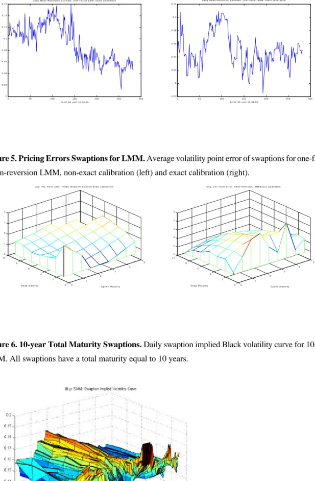
In table 6, we also report the autocorrelation of daily pricing errors for caplets and swaptions. These autocorrelations are quite high for all models, which is an indication of the systematic nature of the pricing errors. There are also maturity effects in the pricing errors for the swaptions, as is shown in figure 5. For the exactly calibrated model, the pricing errors decrease with swap maturity, and swaptions with long swap maturities are underpriced. Also, swaptions with very short or very long option maturities are underpriced. In case of non-exact calibration, swaptions with short and long total maturities are overpriced, whereas swaptions with intermediate total maturities are underpriced. This pricing error pattern is caused by the absence of a humped volatility structure in the non-exact calibration model.

To formally test whether the models on average correctly price caplets and swaptions, we estimate the following regression equation for every swaption separately

where IV_tS,LMM(T_i,T_j) is the implied volatility at day t of the swaption price that is implied by the LMM; similar notation is used for caplets. Using regression equation (15), we thus investigate to what extent the LMM explains the observed difference between swaption and caplet implied volatilities. If the model is correct, "ij is equal to zero and $ij is equal to one. Amin and Morton (1994) estimate the same regression

equation for their analysis of Eurodollar futures options, but they use prices of options instead of implied volatilities. This is an important difference, because prices of options are partially determined by their intrinsic value and the initial term structure, which are the same for the model price and the observed price. This explains why Amin and Morton (1994) find very high R2 _{values, although the models they analyze}

are still rejected statistically. We prefer to use implied volatilities, because the implied volatility of an option is a measure that corrects for the price effects of the intrinsic value and the initial term structure. We choose to use the difference between swaption and caplet volatilities as this difference has a lower autocorrelation than the caplet and swaption implied volatilities itself. In other words, we eliminate a possible ‘trend’ in the implied volatilities. This decreases biases in the parameter estimates that are associated with regressions of this type, see e.g. Bekaert et al. (1997). The regression setup is also such that both exact and non-exact calibration models can be analyzed with this regression.

In table 7, we present a summary of the results for this regression analysis. It follows that all models are clearly rejected; the F-test for "ij = 0 and $ij = 0 rejects much more often than the 5%-confidence level

that is used. If we compare the difference of the parameter estimates with the ‘correct’ parameter values (zero intercept and slope equal to one) and the R2 _{values of the constant volatility LMMs and the}

11

For example, Littermann and Scheinkman (1991) use factor analysis to find that three factors, a level factor, a yield-spread factor and a curvature factor determine interest rate movements.

IV_tS,LMM(T_i,T_j)&_IVS

t (Ti,Tj) '

"_ij % _$

ij,1 Levelt % $ij,2 YldSprt % $ij,3 Curvt % ,ij,t, t'1,..,282

(16)

errors on caplet implied volatilities for the non-exactly calibrated models, the regression results for these models are worse than for the exactly calibrated models.

The relatively low values for the R-squared are remarkable. Apparently, there is a lot of variation in the swaption and caplet prices that cannot be explained by the model, although a part of this variation could be due to measurement errors in the data, caused by the fact that we use quotes for the implied Black volatilities. To analyze to what extent the pricing errors are caused by measurement errors and to what extent they are caused by misspecification of the volatility function or a missing second (and third) factor, we regress the pricing error for every swaption on three variables that describe the shape of the underlying term structure

where we define the level variable as a short maturity interest rate, the yield spread as the difference between interest rates with a long and short maturity, and where curvature is defined as the difference between an interest rate with intermediate maturity and the average of two interest rates with a long and short maturity. A similar regression equation is estimated for every caplet in case of non-exact calibration. Boudoukh et al. (1997) also estimate such a regression equation, and argue that, if there are missing second and third factors that can be associated with respectively the yield spread and the curvature of the yield curve11_{, one should be able to detect this using equation (16). Also, if for example the assumption of}

lognormally distributed interest rates is incorrect, one would expect correlation between the pricing errors and the yield-curve variables.

In table 8, we present the results of this analysis. Indeed, around 30% to 50% of the variation in the pricing errors can be explained by the yield-curve variables, and the hypothesis that there is no correlation between pricing errors and yield-curve variables is almost always rejected. The yield-spread variable is mostly significantly different from zero, the level and curvature variables are often not significant. Hence, one could argue that there is evidence for a missing second factor. In section 6 we investigate the hypothesis of multiple factors in more detail.

5 One-Factor Swap Market Models

12

We have also examined a SMM with a total maturity of 5 years. The empirical results are similar to the results of the 10-year SMM.

(_n,N&n(t) ' e &_6(T n&t)( n,N&n, n'1,...,N&1 (_n,N&n ' IV S_(T n,TN&Tn), if 6 ' 0 (_n,N&n ' IV S_(T n,TN&Tn) 26T_n

1&_exp(&_26T

n)

, if 6 … 0

(17)

compare the results for the different models. We will calibrate the SMM to the set of 10-year total maturity swaptions and investigate the pricing implications of this model for caplets and swaptions with total maturity less than 10 years.

5.1 Calibration Methodology

The SMM is constructed such as to obtain analytical pricing formulas for a certain set of swaptions, and we will estimate the volatility function of the SMM using this set of swaptions, that all have the same total maturity. Then, we can analyze how well the resulting model prices caplets and swaptions that have a smaller total maturity.

For the SMM, the choice for the total maturity is not unique, because, given a choice for this total maturity, only swaptions and caplets with a total maturity smaller than this given total maturity can be priced with the SMM. Therefore, an obvious choice for this total maturity is 10 years, so that all caplets and (almost) all swaptions can be priced with the SMM12_.

In the data, it is not always the case that we observe swaptions with a total maturity of exactly 10 years. For example, we observe the implied Black volatility of a swaption with an option maturity of 1 month and swap maturities of 7 and 10 years. In this case, we follow market practice and linearly interpolate between the 1-month/7-year swaption implied volatility and the 1-month/10-year swaption implied volatility to obtain the implied volatility for the swaption with option maturity 1 month and total maturity 10 years. In figure 6, we plot the resulting implied Black volatilities of the swaptions with a total maturity of 10 years. It follows that this volatility curve takes different shapes through time, both increasing, decreasing and humped shapes.

Similar to the LMM, it is only possible for a SMM to exactly fit swaption implied Black volatilities with a time-homogeneous volatility function if IVS(T_n, 10&_T is increasing with the option maturity

n) Tn

Tn of the swaption. Again, for the swaption implied Black volatilities with total maturities of 10 years, this is not always the case in the data. Therefore, we choose the same form for the volatility function of the SMM as the choice in equations (9)-(13) for the LMM

13

We use the swaptions that can be priced analytically as control variates.

This leads to exact fitting of the implied Black volatilities of the 10-year total maturity swaptions. The non-exactly calibrated Swap Market Models are also specified similar to the non-non-exactly calibrated LMMs. Hence, the 10-year SMM is calibrated, either exact or non-exact, to 10-year total maturity swaptions with option maturities of 1,3 and 6 months, and 1, 1.5, 2, 3, 4 and 5 years.

We both consider a constant volatility SMM and a mean-reversion SMM. For the mean-reversion SMM, the mean-reversion parameter is estimated daily by minimizing the sum of squared differences between observed implied Black volatilities and Black volatilities that correspond to the prices implied by the SMM, where the sum is taken over all instruments that are not priced directly by the SMM, i.e. swaptions with a total maturity smaller than 10 years, and all caplets.

The prices of these caplets and swaptions cannot be determined analytically for the SMM, and thus we use simulation to price these instruments13_{. However, for computational reasons, we use approximate}

analytical formulas for the prices of caplets and swaptions to estimate the mean-reversion parameter. In the appendix, these approximation formulas are given. The difference between the approximation and simulation prices is larger than for the LMM, but is at maximum equal to 0.5 volatility point. Given the estimated mean-reversion value, we use simulation to obtain prices for the caplets and swaptions.

5.2 Estimation and Pricing Results

In table 9, we give the pricing results for the constant volatility SMM. Most remarkable are the large pricing errors for caplets in case of exact calibration. In figure 7, it is shown that especially short-maturity caplets are overpriced substantially. This is the result of a sometimes sharply decreasing volatility function of the SMM for short maturities, as shown in figure 6. This implies that the forward swap rate with a short forward maturity (and 10 year total maturity) has a much larger variance than the forward swap rate (also with 10 year total maturity) that has a forward maturity that is only a little larger. This can only occur if the forward Libor rate that determines the difference between these two forward swap rates has a very high variance. In case of non-exact calibration, the pricing errors for caplets are much smaller and of the same size as the caplet pricing errors of the non-exactly calibrated LMMs. We can therefore again conclude that exact calibration leads to overfitting of the model, and in this case exact calibration results in very large pricing errors for caplets. Furthermore, the average absolute pricing error on 10-year swaptions for the non-exactly calibrated model is around 0.6 volatility points, so that the flat volatility function quite reasonably fits the 10-year swaption implied volatilities.

For <10-year swaptions, the effect of a sharply decreasing volatility function is not as dramatic, because the swaption prices are determined by the variances of several forward Libor rates, so that the impact of the high variances of forward Libor rates with short forward maturities is much smaller. Hence, the differences between the exactly and non-exactly calibrated models are small for swaptions, although the

maximal pricing errors are larger in case of exact calibration. Also, the parameter estimate for the non-exactly calibrated constant volatility SMM is less variable over time than the implied volatilities of the swaptions that are used for the exactly calibrated SMM, as can been seen in tables 4 and 5.

For the constant volatility SMM, the fit on <10-year swaptions is a little worse than the constant volatility LMM, both in the case of exact and non-exact calibration. The constant volatility SMM typically underprices swaptions with total maturities less than 10 years. An explanation for this result is the absence of mean-reversion. This can be seen as follows. Consider the 10-year SMM and suppose we are pricing a swaption with option maturity and swap maturity of 1 year, in other words, a 1x1 swaption. The conditional variance Var(S_1,2(T₁)|ö_t) of the 1x1 forward swaprate that determines this swaption price is roughly determined by the conditional variance, over the first year, of the 1x9 swap rate minus the 2x8 swap rate, Var(S_1,9(T₁)&_S . Mean-reversion will lower the conditional variance over the first

2,8(T1)|öt)

year of the 2x8 swap rate, whereas the conditional variance of the 1x9 swap rate is fixed and determined by the observed implied volatility of the 1x9 swaption. Therefore, the conditional variance of the 1x1 swap rate will increase if mean-reversion is introduced. Hence, the absence of mean-reversion implies that the SMM underprices swaptions.

In figure 4b we plot the mean-reversion parameter estimates for every day in the dataset, and in table 5 we summarize the parameter estimates. As expected, the average mean-reversion estimates are positive, but a little smaller than the reversion estimates for the LMM. Table 9 shows that including reversion leads to a large decrease in absolute pricing errors for swaptions, although the influence of reversion is somewhat smaller than for the LMM. Similar to the constant volatility SMMs, the mean-reversion SMMs have larger absolute pricing errors on the <10-year swaptions than the mean-mean-reversion LMMs. We can thus conclude that the Libor Market Models outperform the Swap Market Models in pricing caplets and swaptions. Barton, Brace and Dun (1998) and Rebonato (1999) show in simulation studies that if the LMM (or the SMM) is the true model, the prices for caps and swaptions implied by the SMM (or the LMM) are quite close to the true prices. In contrast, we show that empirically, calibrating the LMM to caplets leads to very different results than calibrating the SMM to swaptions.

5.3 Analysis of Pricing Errors

In figure 7, we plot the average pricing error per caplet and swaption for the mean-reversion SMMs The maturity effects in the pricing errors of the exact calibration model are similar to the maturity effects in the pricing errors of the non-exact calibration model. We already mentioned above that short-maturity caplets are overpriced by all SMMs. It also follows that swaptions with short total maturities have the largest pricing errors, and these pricing errors are positive on average. The swaptions with longer total maturities are underpriced by the mean-reversion SMM.

14

The results of regression (15) and (16) are not presented for the SMM and the two-factor LMM, as they are similar to the results for the one-factor LMM, but they are available on request.

volatilities on the difference between swaption and caplet implied volatilities that follows from the SMM14_.

In almost all cases the model is statistically rejected. The regression results for the case of non-exact calibration are a little better than for exact calibration. Also, the R2 _{values are smaller than for the LMMs.}

We also estimate the regression of pricing errors for caplets and swaptions on the level, yield spread and curvature in equation (16). Again, between 30% and 50% of the variation in pricing errors is explained by these three yield-curve variables, although on average the explanatory power of these yield-curve variables is smaller than for the LMMs. Hence, although the pricing errors are larger for the SMM, a smaller part of these pricing errors can be explained by the yield-curve variables. Again, the yield-spread is strongly correlated with the pricing errors, which could be an indication for a missing second factor.

6 Two-Factor Libor Market Models

6.1 Calibration Methodology

In the previous sections we have found some indication that a second factor might (partially) explain the pricing errors that were found for the one-factor models. Also, Longstaff, Santa-Clara and Schwartz (1999) conclude that many factors are needed to correctly price American or Bermudan swaptions. However, they only analyze a constant volatility, exact calibration market model. Here, we will analyze whether multi-factor models improve on one-multi-factor models for the pricing of European instruments, even if we include mean-reversion in the first factor and use non-exact calibration. Of course, even if one-factor models suffice for the pricing of European instruments, there are other motivations to examine and use multi-factor models, for example to introduce a non-perfect correlation between contemporaneous interest rate changes, see Rebonato (1998).

We consider some two-factor Libor Market Models in this section. We choose to extend the LMM to a two-factor setting because this model outperforms the SMM in the one-factor setting. The first two-factor model extends the one-factor constant volatility LMM, so that the volatility function of the first factor is given by equation (9) in case of exact calibration and by equation (12) in case of non-exact calibration. The volatility function of the second factor is chosen to be of the exponential type, following Vasicek (1977) and Hull-White (1990), and this second factor is the same for both exact and non-exact calibration

(_1,n(t) ' (

1, non&exact calibration

(_2,n(t) ' _e&6(Tn&t)( 2, n'1,...,N&1 (_1,n(t) ' ₍ 1,n, exact calibration (_2,n(t) ' _e&6(Tn&t)( 2, n'1,...,N&1

(18)

1, non&exact calibration

(_2,n(t) ' ₍ 2, n'1,...,N&1 (_1,n(t) ' _e&6(Tn&t)( 1,n, exact calibration (_2,n(t) ' ( 2, n'1,...,N&1

(19)

In case of exact calibration, the volatility function of the first factor is chosen to exactly fit observed caplet implied volatilities, using the relation T_nIVC(T_n)2 ' , where .

m

Tn

0

(_n(t)y(_n(t)dt (_n(t) ' ₍(

1,n(t), (2,n(t))

In case of non-exact calibration, the parameter (1 is estimated by least squares fitting of caplet implied

volatilities, given values for the other parameters. Both for the exact and non-exact calibration model, the parameters 6 and (2 are estimated by minimizing the sum of squared pricing errors for swaptions, where

the pricing error is again measured in terms of implied Black volatilities.

The second two-factor model that will be analyzed is an extension of the one-factor mean-reversion

LMM, and we extend this model by adding a second factor with a constant volatility function

Again, the parameters 6 and (2 are estimated by minimizing the sum of squared pricing errors for

swaptions, whereas (1 is estimated by least squares fitting of caplet implied volatilities in case of non-exact

calibration.

The two-factor models in (18) and (19) both have one factor that exhibits mean-reversion. In fact, the non-exact calibration models in (18) and (19) are mathematically the same; the difference between these models is whether the parameter (1 or (2 is estimated from the observed caplet implied volatilities.

All two-factor models thus have two parameters that are estimated from swaption prices, and the observed caplet implied volatilities are either exactly matched by the model or fitted with one parameter. Because the number of parameters estimated from swaption prices is the same for all models, this setup enables us to compare both exact versus non-exact calibration and the two-factor models in (18) and (19), by comparing the accuracy in pricing swaptions.

6.2 Estimation and Pricing Results

In table 10 we present the parameter estimates for the two-factor LMMs. For both models of equation (18) and (19), the mean-reversion parameter estimates are larger than for the one-factor models. Hence, the

two-factor models have one two-factor constant volatility two-factor that shifts the entire yield curve, and another two-factor that exhibits relatively fast mean-reversion and therefore primarily influences the short end of the yield curve. This behaviour of two-factor models has also been found by e.g. De Jong (1999). Finally, the parameter estimates of the two-factor models are more volatile over time than the parameter estimates of the one-factor models.

In table 11, the pricing results of the two-factor models are given. The model with the exponential volatility function for the second factor in (18) of course yields lower absolute pricing errors than the one-factor constant volatility LMM, but the pricing errors are still larger than for the one-one-factor mean-reversion LMM. It turns out that the influence of the mean-reversion parameter in this two-factor model is not as straightforward as in the one-factor reversion model; swaption prices are first decreasing in the mean-reversion parameter in (18), but at some value of this parameter swaption prices become an increasing function of this mean-reversion parameter. Therefore, there is still overpricing of swaptions in this two-factor model, especially for the swaptions with long swap maturities.

For the model with the constant volatility function for the second factor in equation (19), the pricing errors are only reduced by 0.1 volatility point relative to the one-factor mean-reversion LMM. Therefore, we can conclude that, if we already include mean-reversion in the first factor, adding a second additive factor to the LMM is not necessary for the pricing of caplets and swaptions. An important difference between one- and two-factor models is the fact that interest rates of different maturities are not perfectly correlated in a two-factor model. Although swaption prices do depend on this correlation between interest rates of different maturities, this turns out to be a second order effect; swaption prices are primarily determined by the volatilities of interest rates. This is in contrast with the findings of Longstaff, Santa-Clara, and Schwartz (1999). We have two explanations for this difference in results. First, Longstaff, Santa-Clara, and Schwartz only analyze a constant volatility, exact calibration market model, and we have shown that these models yield much higher pricing errors than mean-reversion, non-exact calibration models, so that Longstaff, Santa-Clara, and Schwartz might overestimate the relevant number of factors. Second, Longstaff, Santa-Clara, and Schwartz analyze American swaptions, whereas we analyze European instruments, and it could be that including multiple factors is especially important for the pricing of American swaptions. Further research is required to resolve this issue.

6.3 Analysis of Pricing Errors

The pricing errors of the two-factor models are close to the pricing errors of the one-factor models, and the results for the specification test in equation (15) are similar to the one-factor results. Again, all models are statistically rejected. The R2 _{values are lower than for the one-factor models, whereas the slope coefficients}

in (15) are closer to one for the two-factor models, but the differences with the one-factor models are small. The results for regression (16) show that for the two-factor models, the yield spread variable is still strongly correlated with the pricing errors. The curvature variable is a little more significant than for the

one-factor models. These results imply that the pricing errors still contain some systematic patterns, which are not captured by the models that we have analyzed. From the results for the two-factor models we can conclude that it is unlikely that we have used a too low number of (additive) factors.

7 Conclusions

In this paper, we empirically examine a recently developed class of models to price interest rate derivatives, the so-called market models of interest rates. This class of models has several advantages over the traditional approach of Heath, Jarrow, and Morton (1992). First, these models are based directly on observable market rates, such as Libor rates and swap rates, instead of instantaneous (forward) interest rates. Second, the models yield pricing formulas for caplets or swaptions that correspond to the Black pricing formulas that are used in practice. And third, as a consequence, these models can easily be calibrated to market prices of caps or swaptions.

We analyze and compare two one- and two-factor market models: the Libor Market Model (LMM), developed by Miltersen, Sandmann, and Sondermann (1997) and Brace, Gatarek, and Musiela (1997), and the Swap Market Model (SMM), introduced by Jamshidian (1997) and Musiela and Rutkowski (1998). We analyze constant volatility and mean-reversion specifications of the models. We also consider two calibration methodologies, exact calibration, that leads to exact fitting of a set of derivative prices, and non-exact calibration, that does not lead to such an non-exact fit.

We show that a constant volatility specification for the LMM leads to overpricing of all swaptions. Including a mean-reversion term in the volatility specification typically increases the fit of the LMM, and the estimates for the strength of mean-reversion are quite stable over time. For this model