A construction of continuous-time ARMA models by iterations of Ornstein-Uhlenbeck processes

Transactions

[email protected] ISSN: 1696-2281

eISSN: 2013-8830 www.idescat.cat/sort/

A construction of continuous-time ARMA models

by iterations of Ornstein-Uhlenbeck processes

Argimiro Arratia1, Alejandra Caba˜na2and Enrique M. Caba˜na3

Abstract

We present a construction of a family of continuous-time ARMA processes based onpiterations of the linear operator that maps a L ´evy process onto an Ornstein-Uhlenbeck process. The con-struction resembles the procedure to build an AR(p) from an AR(1). We show that this family is in fact a subfamily of the well-known CARMA(p,q) processes, with several interesting advantages, including a smaller number of parameters. The resulting processes are linear combinations of Ornstein-Uhlenbeck processes all driven by the same L ´evy process. This provides a straightfor-ward computation of covariances, a state-space model representation and methods for estimating parameters. Furthermore, the discrete and equally spaced sampling of the process turns to be an ARMA(p,p−1) process. We propose methods for estimating the parameters of the iterated Ornstein-Uhlenbeck process when the noise is either driven by a Wiener or a more general L ´evy process, and show simulations and applications to real data.

MSC: 60G10, 62M10, 62M99 60M99.

Keywords: Ornstein-Uhlenbeck process, L ´evy process, Continuous ARMA, stationary process.

1. Introduction

The link between discrete time autoregressive moving average (ARMA) processes and stationary processes with continuous-time has been of interest for many years, see for in-stance, Doob (1944), Durbin (1961), Bergstrom (1984, 1996) and more recently Brock-well (2009), Thornton and Chambers (2013). Continuous time ARMA processes are better suited than their discrete counterparts for modelling irregularly spaced data, and when the white noise is driven by a non-Gaussian process it becomes a more realistic model in finance and other fields of application.

1_{Universitat Polit`ecnica de Catalunya, Barcelona, Spain. [email protected]}

Supported by Spain’s MINECO project APCOM (TIN2014-57226-P) and Generalitat de Catalunya 2014SGR 890 (MACDA).

2_{Universitat Aut`onoma de Barcelona, Spain. [email protected]} Supported by Spain’s MINECO project MTM2015-69493-R.

3_{Universidad de la Rep´ublica, Montevideo, Uruguay. [email protected]} Received: November 2015

A popular continuous-time representation of ARMA(p,q) process (known as CARMA(p,q)) can be obtained via a state-space representation of the formal equation

a(D)Y(t) =σb(D)DΛ(t),

where σ>0 is a scale parameter,D denotes differentiation with respect to t, Λ is a second-order L´evy process,a(z) =zp+a1zp−1+. . .+apis a polynomial of orderpand

b(z) =b0+b1z+. . .+bqzqa polynomial of orderq≤p−1 with coefficientbq6=0 (see,

e.g., Brockwell, 2004, 2009, Thornton and Chambers, 2013). The parameters of this model are estimated by adjusting first an ARMA(p,q),q<pto regularly spaced data. Then obtain the parameters of the continuous version whose values at the observation times have the same distribution of the fitted ARMA. Hence,p+q+1 parameters have to be estimated.

We propose in this work a parsimonious model for continuous autoregression, with fewer parameters (as we shall see exactly p plus the variance). Our construction de-parts from the observation that a Ornstein-Uhlenbeck (OU) process can be thought of as continuous-time interpolation of an autoregressive process of order one (i.e. an AR(1)). This is shown in Section 2, where we also review some well known facts on L´evy pro-cesses, ARMA models and their representations. The model is obtained by a procedure that resembles the one that allows to build an AR(p) from an AR(1). Departing from this analogy, we define and analyse the result of iterating the application of the operator that maps a Wiener process onto an OU process. This operator is defined in Section 3 and denotedOU_{, with subscripts denoting the parameters involved.}

The p iterations of OU_{, for each positive integer p, give rise to a new family of} processes, the Ornstein-Uhlenbeck processes of orderp, denoted OU(p). They can be used as models for either stationary continuous-time processes or the series obtained by observing these continuous processes at equally spaced instants. We show that an OU(p) process can be expressed as a linear combination of ordinary OU processes, or generalized OU processes, also defined in Section 3. This result resembles the aggrega-tions of Gaussian (and non-Gaussian) processes studied with the idea of deconstructing a complicated economic model into simpler constituents. In the extensive literature on aggregations (or superpositions) of stochastic processes the aggregated processes are driven by independent L´evy processes (see, e.g., Granger and Morris, 1976, Granger, 1980, Barndorff-Nielsen, 2001, Eliazar and Klafter, 2009, among many others). A dis-tinctive point of our construction is that the stochastic processes obtained by convolution of the OU operator result in a linear combination comprised of processes driven by the same L´evy process.

Another consequence of writing the OU(p) process as the aggregation of simpler ones is the derivation of a closed formula for its covariance. This has important practical implications since it allows to easily estimate the parameters of a OU(p) process by matching correlations (a procedure resembling the method of moments, to be described in Section 6.2), and by maximum likelihood.

In Section 4 we show how to write the discrete version of a OU(p) as a state-space model, and from this representation we show in Section 5 that for p>1, a OU(p) be-haves like an aggregation of AR processes (in the manner considered in Granger and Morris (1976)), that turns out to be an ARMA(p,q), withq≤p−1. Consequently the OU(p) processes are a subfamily of the CARMA(p,q)processes. Notwithstanding this structural similarity, the family of discretized OU(p) processes is more parsimonious than the family of ARMA(p,p−1) processes, and we shall see empirically that it is able to fit well the autocovariances for large lags. Hence, OU processes of higher order appear as a new continuous model, competitive in a discrete time setting with higher order autoregressive processes (AR or ARMA). The estimation of the parameters of OU(p) processes is attempted in Section 6. Simulations and applications to real data are provided in Section 6.5. Our concluding remarks are in Section 7.

2. Preliminaries

Let us recall that a L´evy processΛ(t)is a c`adl`ag function, with independent and station-ary increments, that vanishes int=0. As a consequence,Λ(t)is, for eacht, a random variable with an infinitely divisible law (Sato, 1999). A Wiener processW is a cen-tred Gaussian process, with independent increments and variance E(W(t)−W(s))2₌ σ2_{|t−s|. Wiener processes are the only L´evy processes with almost surely} continu-ous paths. For parameterλ>0 the classical Ornstein-Uhlenbeck process is defined as

Rt

−∞e−λ(t−s)dW(s)(Uhlenbeck and Ornstein, 1930).

Wiener process can be replaced by a second order L´evy processΛto define a L´evy driven Ornstein-Uhlenbeck process as

x(t)(=xλ,Λ(t)):=

Z t

−∞e

−λ(t−s)_{dΛ(s) (1)}

The previous equation can be formally written in differential form

dx(t) =−λx(t)dt+dΛ(t) (2)

We may think ofxas the result of accumulating a random noisedΛ_{, with reversion to}

the mean (that we assume to be 0) of exponential decay with rateλ.

When the Ornstein-Uhlenbeck processxis sampled at equally spaced times{hτ:h=

0,1,2, . . . ,n},τ>0, the seriesXh=x(hτ)obeys an autoregressive model of order 1 (i.e.

an AR(1)), becauseXh+1=e−λτXh+Zh+1, whereZh+1=

Z (h+1)τ

hτ

e−λ((h+1)τ−s)dΛ(s), is the stochastic innovation.

Hence, we can consider the OU process as continuous-time interpolation of an AR(1) process. Notice that both models are stationary. This link between AR(1) and OU(1) suggests the definition of iterated OU processes introduced in Section 3.

An ARMA(p,q) or autoregressive moving average process of order (p,q) has the following form

xt=φ1xt−1+· · ·+φpxt−p+θ0ǫt+θ1ǫt−1+· · ·+θqǫt−q

whereφ1, . . . ,φp are the autoregressive parameters,θ0, . . . ,θqare the moving average

parameters, and the white-noise processǫt has variance one. Denote byBthe backshift

operator that carriesxt intoxt−1. By considering the polynomials in the backshift oper-ator,

φ(B) =1−φ1B− · · · −φpBp and θ(B) =θ0+θ1B+· · ·+θqBq

the ARMA(p,q)model can be written as

φ(B)xt=θ(B)ǫt (3)

This compact expression comes in handy for analysing structural properties of time series. It also links to the representation of ARMA processes as astate-space model, useful for simplifying maximum likelihood estimation and forecasting. A state-space model has the general form

Yt =AYt−1+ηηηt (4)

xt=KTYt+Nt (5)

where (4) is the state equation and (5) is the observation equation, with Yt the m

-dimensional state vector,AandKarem×mandm×kcoefficient matrices,KTdenotes the transpose ofK,ηηηandNaremandkdimensional white noises.Nwould be present only if the processxtis observed subject to additional noise (see Box, Jenkins, and

Rein-sel, 1994 for further details). We present in Section 4 a state-space model representation of our generalized OU process.

3. Ornstein-Uhlenbeck processes of order

p

p

p

The AR(1) process Xt =φXt−1+ǫt, where ǫt, t∈Z, is a white noise, can be written

as (1−φB)Xt =ǫt using the back-shift operator B. Equivalently, Xt can be written

asXt =MA1/ρǫt, whereMA1/ρ is the moving average that mapsǫt ontoMA1/ρǫt,=

P∞

j=0 1

Moreover, the AR(p) processXt = p X j=1 φjXt−j+ǫt ( orφ(B)Xt=ǫt), whereφ(z) = 1− p X j=1 φjzj= p

∏

(1−z/ρj)has rootsρj=eλj,j=1, . . . ,p, can be obtained by applying

the composition of the moving averagesMA_1/ρ

jto the noise, that is:

Xt= p

∏

Now consider the operatorMA_e−λthat mapsǫ_t onto

MA_e−λǫt =

X

l≤t,integer

e−λ(t−l)ǫl

A continuous version of this operator isOU_{λthat mapsy(t),t∈Ronto}

OU_{λy(t) =}

Z t

−∞e

−λ(t−s)_{dy(s), (6)}

whenever the integral can be defined. The definition of OU_{λ is extended to include} complex processes, by replacingλbyκ=λ+iµ,λ>0,µ∈Rin (6). The set of complex numbers with positive real part is denoted byC+, and the conjugate ofκis denoted by

¯ κ.

Forp≥1 and parametersκκκ= (κ1, . . . , κp), the previous argument suggests to define the following process obtained as repeated compositions of operatorsOU_κ

j, j=1, . . . ,p: OU_κκκy(t):=OU_κ 1OUκ2· · ·OUκpy(t) = p

∏

This is calledOrnstein-Uhlenbeck process of order p with parametersκκκ= (κ1, . . . , κp)∈

(C+)p_{. The composition∏}p

j=1OUκj is unambiguously defined because the application

ofOU_κ

j operators is commutative as shown in Theorem 1(i) below.

The particular case of interest where the underlying noise is a second order L´evy processΛ, namely, OU_κκκΛ(t):=OU_κ 1OUκ2· · ·OUκpΛ(t) = p

∏

is called theL´evy-driven Ornstein-Uhlenbeck process of order p with parametersκκκ= (κ1, . . . , κp)∈(C+)p.

For technical reasons, it is convenient to introduce theOrnstein-Uhlenbeck operator

OU(_κh)_{of degree h with parameterκthat mapsyonto}

OU(_κh)_{y(t) =} Z t −∞e −κ(t−s)(−κ(t−s))h h! dy(s) (9) andΛonto ξ(h) κ (t) = Z t −∞ e−κ(t−s)(−κ(t−s)) h h! dΛ(s) (10)

We call the process (10) generalized Ornstein-Uhlenbeck process of order 1 and degreeh. For the remainder of the paper we restrict the underlying noise to a second order L´evyΛ_{, but note that the general properties of the}OU_{κoperator that we are going} to show hold for any random functiony(t)for which the integral (6) is defined.

3.1. Properties of the operatorOUOUOU_κκκ

The following statements summarize some properties of products (compositions) of the operators defined by (7) and (9), and correspondingly, of the stationary centred processes ξ(κh), h≥0. In particular, the Ornstein-Uhlenbeck processes of order 1 and degree 0,

ξ(κ0)=ξκare the ordinary Ornstein-Uhlenbeck processes (1).

Theorem 1

(i) Whenκ16=κ2, the productOUκ2OUκ1 can be computed as

κ1 κ1−κ2 OU_κ 1+ κ2 κ2−κ1 OU_κ 2

and is therefore commutative. (ii) The composition∏p_j=1OU_κ

jconstructed with pairwise differentκ1, . . . , κpis equal

to the linear combination

p

∏

(iii) For i=1,2, . . .,OU_κOU(_κi)₌OU(_κi)_−κOU(_κi+1)_.

(iv) For any positive integer p the p-th power of the Ornstein-Uhlenbeck operator has the expansion OU_κp₌ p−1 X j=0 p−1 j OU(_κj)_{. (13)}

(v) Letκ1, . . . , κqbe pairwise different complex numbers with positive real parts, and

p1, . . . ,pqpositive integers, and let us denote byκκκa complex vector in(C+)pwith

componentsκhrepeated ph times, ph≥1, h=1, . . . ,q,

Pq h=1ph=p. Then, with Kh(κκκ)defined by (12), q

∏

An immediate consequence is that the operatorOU_{κκκ with p-vector parameterκ}κκcan be written as a linear combination of poperatorsOU_{κ or}OU(_κh) _{for suitable scalar values} κand non-negative integerh. Therefore, the process OU_κκκΛ can be written as a linear combination of OU processes driven by the same L´evy process, as stated in the following Corollary.

Corollary 1

(i) The processOU_κκκ(Λ) = q

∏

h=1 OUph

κh(Λ)can be expressed as the linear combination

OU_κκκ(Λ) = q X h=1 Kh(κκκ) p_h−1 X j=0 p_h−1 j ξ(κjh) (14)

of the p processes{ξκ(j_h):h=1, . . . ,q,j=0. . . ,ph−1}(see (10)).

(ii) Consequently, OU_κκκΛ(t) = q X h=1 Kh(κκκ) p_h−1 X j=0 p_h−1 j Rt −∞e−κh(t−s) (− κh(t−s))j j! dΛ(s)

Corollary 2 For realλ, µ, withλ>0, the productOU_λ+iµOU_{λ−iµis real, that is,}

ap-plied to a real process produces a real image.

3.2. Computing the covariances The representation x:=OU_κκκ(Λ) = q X h=1 Kh(κ) p_h−1 X j=0 ph−1 j OU(_κj) h(Λ)

ofx as a linear combination of the processesξ(κih)=OU

(i)

κh(Λ) allows a direct

compu-tation of the covariancesγ(t) =Ex(t)x¯(0) through a closed formula, in terms of the covariancesγ(i1,i2) κ₁,κ₂(t) =Eξκ(i₁1)(t)ξ¯κ(i₂2)(0): γ(t)= q X h′₌₁ p_h′−1 X i′₌₀ q X h′′₌₁ p_h′′−1 X i′′₌₀ Kh′(κκκ)K¯h′′(κκκ) ph′−1 i′ ph′′−1 i′′ γκ(i_h′,′i,′′κ)h′′(t) (15) withv2=VarΛ(1), γ(i₁,i₂) κ1,κ2(t) =v 2_(−κ 1)i1(−κ¯2)i2 Z 0 −∞ e−κ1(t−s)(t−s) i1 i1! e −κ¯₂(−s)(−s)i2 i2! ds =v2(−κ1)i1(−κ¯2)i2e−κ1t i1 X j=0 i1 j tj i1!i2! Z 0 −∞e (κ1+κ¯2)s_(−s)i1+i2−j_ds =v 2_(−κ 1)i1(−κ¯2)i2e−κ1t i2! i₁ X j=0 tj_(i 1+i2−j)! j!(i1−j)!(κ1+κ¯2)(i1+i2−j+1) (16)

A real expression for the covariance when the imaginary parameters appear as conjugate pairs can be obtained but it is much more involved than this one.

4. The OU(

p

p

p

) process as a state-space model

Theorem 1 and its corollaries lead to express the OU(p) process by means of linear state-space models. The state-space modelling provides a unified methodology for the analysis of time series (see Durbin and Koopman, 2001).

In the simplest case, where the elements ofκκκ are all different, the process x(t) =

OU_κκκΛ(t)is a linear combination of the state vectorξξξκκκ(t) = (ξκ1(t), ξκ2(t), . . . , ξκp(t))

T_, whereξκ_j=OUκ_j(Λ).

More precisely, the vectorial process

ξξξκκκ(t) = (ξκ1(t), ξκ2(t), . . . , ξκp(t))

T_{, ξ}

κj=OUκj(Λ)

andx(t) =OU_κκκΛ(t)satisfy the linear equations

ξξξκκκ(t) =diag(e−κ1τ,e−κ2τ, . . . ,e−κpτ)ξξξκκκ(t−τ) +ηηηκκκ,τττ(t) (17) and x(t) =KKKT(κκκ)ξξξ(t), (18) ηηηκκκ,τττ(t) = (ηκ1,τ(t), ηκ2,τ(t), . . . , ηκp,τ(t)) T , ηκj,τ(t) = Z t t−τe −κj(t−s)_dΛ(s), Var(ηηηκκκ,τττ(t)) =v2((vj,l)), vj,l= Z t t−τ e−(κj+κ¯l)(t−s)_ds=1−e −(κ_j+κ¯_l)τ κj+κ¯l (19)

and the coefficients from (12),KKKT

(κκκ) = (K1(κκκ),K2(κκκ), . . . ,Kp(κκκ)).

The initial valueξξξ(0) is estimated by means of its conditional expectation ˆξξξ(0) =

E(ξ(0)|x(0)) =KKKT(κκκ)V x(0) K K KT(κκκ)V KKK , withV =Var(ξξξ(0)) = 1 κj+κ¯l .

An application of Kalman filter to this state-space model leads to compute the likeli-hood ofxxx= (x(0),x(τ), . . .,x(nτ)). Some Kalman filter programs included in software packages require the processes in the state-space to be real. That condition is not ful-filled by the model described by equations (17) and (18). An equivalent description by means of real processes can be obtained by ordering the parametersκκκwith the imaginary components paired with their conjugates in such a way thatκ2h=κ¯2h−1,h=1,2, . . . ,c and the imaginary componentℑ_{(κj) =0 if and only if 2c< j≤p.}

Then the matrixM= ((Mj,k))with all elements equal to zero exceptM2h−1,2h−1=

M2h−1,2h=1,−M2h,2h−1=M2h,2h=i, h=1,2, . . . ,candMj,j=1,2c< j≤p, induces

the linear transformationξξξ7→Mξξξthat leads to the new state-space description

Mξξξ(t) =Mdiag(e−κ1τ_,e−κ2τ_{, . . . ,e}−κpτ_)M−1_{Mξξξ(t−τ) +Mηηη(t), (20)}

x(t) =KKKTM−1Mξξξ(t), (21)

Observe that there is no loss of generality in choosing the spacingτ between obser-vations as unity for the derivation of the state-space equations. Hence, we setτ =1 in the sequel and, in addition,τ will be omitted from the notation.

Whenκ1, . . . , κq are all different, p1, . . . ,pqare positive integers,

Pq

h=1ph =pand κ

κκ is a p-vector with ph repeated components equal to κh, the OU(p) process x(t) =

OU_κκκΛ(t)is a linear function of the state-space vector

ξ(0) κ1, ξ (1) κ1, . . . , ξ (p₁−1) κ1 , . . . , ξ (0) κq, ξ (1) κq, . . . , ξ (pq−1) κq

where the components are given by (10), and the transition equation is no longer ex-pressed by a diagonal matrix. In this case the state-space model has the following form

ξξξ(t) =Aξξξ(t−1) +ηηη(t)

x(t) =KKKTξξξ(t) (22)

We leave the technical details of this derivation to Appendix B. The termsξξξ(t),A,ηηη(t)

andKKK are precisely defined in (36). The real version of (22), when the processξξξ has imaginary components is obtained by multiplying both equations by a block-diagonal matrixC (which is defined precisely in the Appendix), giving us the real state-space model

Cξξξ(t) = (CAC−1)(Cξξξ(t−1)) +Cηηη(t), (23)

x(t) = (KKKT

C−1)(Cξξξ(t)). (24)

5. The OU(

p

p

p

) as an ARMA(

p

p

p

,

p

p

p

−

−

−

1

1

1)

The studies of properties of linear transformations and aggregations of similar processes have produced a great amount of work stemming from the seminal paper by Granger and Morris (1976) on the invariance of MA and ARMA processes under these operations. These results and extensions to vector autoregressive moving average (VARMA) pro-cesses are compiled in the textbook by L¨utkepohl (2005).

The description of the OU(p) process x=OU_κκκ(Λ) with parameters κκκ as a linear state-space model, given in the previous section, will allow us to show that the series

x(0), x(1),. . ., x(n) satisfies an ARMA(p,q) model with q smaller than p. We refer

the reader to (L¨utkepohl, 2005, Ch. 11) for a presentation on VARMA processes and, in particular, to the following result on the invariance property of VARMA processes under linear transformations, which we quote with a minor change of notation:

Theorem 2 (L¨utkepohl, 2005, Cor. 11.1.2)Let y(t)be a d-dimensional, stable, invert-ible VARMA(p,˜q) process and let˜ Fbe an(m×d) matrix of rank m. Then the process zt=Fyt has a VARMA(pˇ,q) representation withˇ pˇ≤(d−m+1)p and˜ qˇ≤(d−m)p˜+q.˜

Equation (23) shows thatCξξξ(t)is ap-dimensional autoregressive vector (ap -dimen-sional VARMA(1,0) process) and Equation (24) expressesx(t)as a linear transformation ofCξξξ(t)by the(1×p)matrixF=KKKT

C−1. Using Theorem 2 (withd=p, ˜p=1, ˜q=0,

m=1) we conclude that(x(t):t=0,1, . . . ,n)is an ARMA( ˇp, ˇq) process with ˇp≤pand ˇ q≤p−1: x(h) = p X j=1 φjx(h−j) + p−1 X l=0 θlǫh−l (25)

whereǫis a Gaussian white noise with variance 1 and the parametersφφφ= (φ1, . . . , φp)T,

θθθ= (θ0, . . . , θp−1)Tof the ARMA process are functions of the parametersκκκof the OU

process. When the noise is any other second order L´evy process the corresponding OU(p)process has the same covariances as the process (25).

By using the backshift operatorB, and the polynomialsφ(z) =1−Pp

j=1φjzj,θ(z) =

Pp−1

l=0θlz

l_{, (25) is written as}

φ(B)x=θ(B)ǫ. (26)

5.1. Identifying the ARMA(ppp,ppp−−−111) from a given OU(((ppp)))process

We proceed now to identify the coefficientsφφφ∈Rpandθθθ∈Rp−1of the ARMA(p,p−1)

model that has the same autocovariances asx=OU_κκκ(Λ).

Case 1.Consider first that all components ofκκκ are pairwise different, and hencex(t)

=Pp

j=1Kjξκj(t)is a linear combination of the OU(1) processes

ξκj(t) = Z t −∞e −κj(t−s)_{dΛ(s) =e}−κj_ξ κj(t−1) + Z t t−1 e−κj(t−s)_dΛ(s)

with innovationsηηηκκκwith componentsηκj(t) =

Rt

t−1e−κj(

t−s)_dΛ(s). For each j, the seriesξκj= (ξκj(h))h∈ZZZsatisfies the AR(1) model

(1−e−κj_B)ξ

(see (17)), and from (18) the seriesx= (x(h))h∈ZZZfollows the ARMA model p

∏

∏

The sum of moving averages in the right-hand term is distributed as the moving average

ζ=

p−1

X

h=0 θhBhǫ

whereǫis a white noise with variance one and the coefficientsθh are suitably chosen.

It is readily verified that the autocovariancescl =Eζ(h)ζ¯(h−l) of this MA are the

coefficients in the sum of powers ofz

p−1 X h=0 θhzh ! p−1 X k=0 ¯ θkz−h ! = p−1 X l=−p+1 clzl. (27)

A similar formula that takes into account the correlations (19) between the noises ηκ_kindicates that the same autocovariances are given by the identity

J(z):= p X j=1 p X l=1 KjK¯lGj(z)G¯l(1/z)vj,l= p−1 X l=−p+1 clzl (28) whereGj(z) =∏l6=j(1−e−κlz) = Pp−1 l=0gj,lz l_.

The coefficientsgj,l and the functionJare completely determined from the

parame-ters of the OU process. In order to express the parameparame-ters of the ARMA(p,p−1) process in terms ofκκκandv2=VarΛ(1)it remains to obtain the coefficientsθhin the factorization

(27). The rootsρj(j=1,2, . . . ,p−1)of θ(z) = p−1 X h=0 θhzh=θ0 p−1

∏

are obtained by choosing the roots of the polynomialzp−1_{θ(z)θ¯(1/z) =z}p−1_J(z)with modules greater than one (the remaining roots are their inverses). Then allθhare written

in terms of theρh and the size factorθ0 by applying (29). The value ofθ0 follows by using an additional equation, namely, the equality of the terms of degree zero inJ(z)

p−1 X l=0 |θl|2= p X j=1 p X l=1 KjK¯lvj,l p−1 X h=0 gj,hg¯l,h.

The general result, for arbitraryκκκ is much more involved and its derivation is de-ferred to Appendix C.

6. Estimation of the parameters of OU(

p

p

p

)

6.1. Reparameterization by means of real parameters

Our purpose is to insert the expression (15) for the covariance γ(t) of the process

x(t) =OU_κκκΛ(t) in a numeric optimization procedure in order to compute the maxi-mum likelihood estimates of the parameters. Althoughγ(t)depends continuously onκκκ, the same does not happen with each term in the expression (15), because of the lack of boundedness of the coefficients of the linear combination when two different values of the components ofκκκapproach each other. Since we wish to consider real processesx

and the process itself and its covarianceγ(t) depend only of the unordered set of the components ofκκκ, we shall reparameterize the process. For the sake of simplicity, but without losing generality, consider the case where the components in κκκ are pairwise different. LetKj,i= _(−κ 1

j)i∏l6=j(1−κl/κj) (in particular,Kj,0 is the same asKj). Then the

processesxi(t) =Pp

j=1Kj,iξj(t)and the coefficientsβββ= (β1, . . . , βp)of the polynomial

g(z) = p

∏

The resulting process is real, because of Corollary 2. This works likewise for the general case ofκκκwith some repetitions. Therefore the new parameterβββshall be adopted. 6.2. Matching correlations estimation (MCE)

From the closed formula (15) for the covarianceγ and the relationship (30) betweenκκκ andβββ, we have a mapping(βββ,v2_{)7→γ(t), for eacht. Since}

does not depend onv2, these equations determine a mapC_{:(βββ,T)7→ρρρ}(T)_=C(βββ,T) for eachT. After choosing a value ofT and obtaining an estimateρρρ(eT)ofρρρ(T)based on

the empirical covariances ofx, we propose as a first estimate ofβββ, the vector ˇβββT such

that all the components of the correspondingκκκhave positive real parts, and such that the Euclidean normkρρρ(eT)−C(βββˇT,T)kreaches its minimum. The procedure resembles the

estimation by themethod of moments. The components ofρρρ(eT)for the series(xj)j=1,2,...,n

are computed as ρe,h=γe,h/γe,0, γe,h= 1 n n−h X j=1 xjxj+h.

6.3. Maximum likelihood estimation (MLE) in the Gaussian case

In this case x(t) =OU_{κκκσW(t), whereW(t) is standard Wiener process. Assume that}

x(t)is observed at times 0, τ ,2τ, . . . ,nτ. By choosingτ the time unit of measure, as in Section 4, we assume without loss of generality that our observations arexxx= (x(0),x(1), . . . ,x(n))T_.

The likelihoodLof the vectorxxxis given by

logL(xxx;βββ, σ2_{) =−}n 2log(2π)− 1 2log(det(ΓΓΓ(βββ, σ 2₎₎₋1 2xxx T_{(ΓΓΓ(βββ, σ}2₎₎−1_xxx

whereΓΓΓhas componentsΓ_h,j=γ(|h−j|)(h,j=0,1, . . . ,n). The Kalman filter associ-ated to the dinamical state-space model in Section 4 provides an efficient alternative to compute the likelihood.

From these elements, a numerical optimization leads to obtain the maximum likeli-hood estimators ˆβββofβββand ˆσ2_ofσ2_{. If required, the estimations ˆκκκfollow by solving the} analogue of the polynomial equation (30) written in terms of the estimators:

p

∏

The optimization for largenand the solution of the algebraic equation for largep re-quire a considerable computation effort, but there are efficient programs to perform both operations, such asoptimandpolyrootinR(R Core Team, 2015). An alternative when the observed process is not assumed to be centred, is to maximize the log-likelihood of

∆xxx= (x(1)−x(0),x(2)−x(1), . . .,x(n)−x(n−1))given by logL(xxx;βββ, σ2_{) =−}n 2log(2π)− 1 2log(det(V(βββ, σ 2₎₎₋1 2∆xxx T_{(V(βββ, σ}2₎₎−1_∆xxx

withV(βββ, σ2_{)equal to then×nmatrix with components}

Vh,j=2γ(|h−j|)−γ(|h−j|+1)−γ(|h−j| −1)

that reduce to 2(γ(0)−γ(1))at the diagonalh= j.

The optimization procedures require an initial guess about the value of the parame-ter to be estimated. The estimators obtained by matching correlations described in the previous section can be used for that purpose.

6.4. The Gaussian case: examples

WhenΛis a Wiener processW, the OU process of order pbelongs to a subclass with

p+1 parameters of the classical family of the 2p-parameters Gaussian ARMA(p,p−1)

xt=φ1xt−1+· · ·+φpxt−p+θ0ǫt+θ1ǫt−1+· · ·+θp−1ǫt−p+1

whereφ1, . . . ,φpandθ0, . . . ,θqare parameters andǫt is a Gaussian noise with variance

1. The parametersκκκ, σ2_{determine the Gaussian likelihood ofOU}

κ κ

κσW, and are estimated

by the values ˆκκκand ˆσ2_{that maximize that likelihood.}

We have observed in several examples that the covariances of the process with the maximum likelihood estimators as parameters, follow closely the empirical covariances of the series. We have simulated the sample paths for the Wiener-driven OU(p) for different values of the parameters.

In the examples below we present simulated series x(j),j=0,1,2, . . . ,n obtained from an OU processx for n=300 and three different values of the parameters and computed the MC and ML estimators ˇβββT, and ˆβββ. The value ofT for the MC estimation

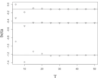
has been arbitrarily set equal to the integral part of 0.9·n, but the graphs of ˇβββT for several

values ofT show in each case that afterT exceeds a moderate threshold, the estimates remain practically constant. One of such graphs is included below (see Figure 2). It is of interest to perform further comparisons of these two methodologies for parameter estimation. A recent antecedent of this kind of comparisons and its importance can be found in Nieto, Orbe and Zarraga (2014).

The simulations show that the correlations of the series with the estimated parameters are fairly adapted to each other and to the empirical covariances. The departure from the theoretical covariances ofxcan be ascribed to the simulation intrinsic randomness.

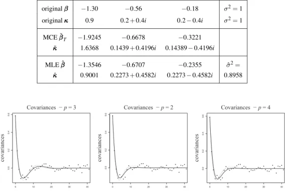
Our first two examples describe OU(3) processes with arbitrarily (and randomly) chosen parameters and the third one imitates the behaviour of Series A that appears in Section 6.5.

Example 1. A series(xh)h=0,1,...,nofn=300 observations of the OUκκκprocessxof order p=3,κκκ= (0.9,0.2+0.4i,0.2−0.4i)andσ2_{=1 was simulated, and the parametersβββ=}

(−1.30,−0.56,−0.18)andσ2_{=1 were estimated by means of matching correlations:} ˇ

β β

βT = (−1.9245,−0.6678,−0.3221),

withT =270; and maximum likelihood:

ˆ

βββ= (−1.3546,−0.6707,−0.2355)

and ˆσ2_{=0.8958. The corresponding estimators forκκκare ˇκκκ= (1.6368,0.1439+0.4196i,} 0.14389−0.4196i)and ˆκκκ= (0.9001, 0.2273+0.4582i, 0.2273−0.4582i).

The following table summarizes the different estimations of this OU(3) process.

originalβββ −1.30 −0.56 −0.18 σ2=1 originalκκκ 0.9 0.2+0.4i 0.2−0.4i σ2=1 MCE ˇβββT −1.9245 −0.6678 −0.3221 ˇ κ κ κ 1.6368 0.1439+0.4196i 0.14389−0.4196i MLE ˆβββ −1.3546 −0.6707 −0.2355 σˆ2= ˆ κ κ κ 0.9001 0.2273+0.4582i 0.2273−0.4582i 0.8958 0 10 20 30 40 0 .0 0 .2 0 .4 0 .6

Covariances −p= 3 Covariances −p= 2 Covariances −p= 4

covariances 0 10 20 30 40 0.0 0.2 0.4 0.6 covariances 0 10 20 30 40 0.0 0.2 0.4 0.6 covariances

Figure 1: Empirical covariances (◦) and covariances of the MC (—) and ML (- - -) fitted OU models, for p=3,2and4corresponding to Example 1. The covariances of OUκκκare indicated with a dotted line.

Figure 1 describes the theoretical, empirical and estimated covariances ofxunder the assumptionp=3, that is, the actual order ofx. The results obtained when the estimation is performed forp=2 and p=4 are also shown. Figure 2 shows that the MC estimates ofβββbecome stable forT moderately large, and close to the already indicated estimations forT =270 (the horizontal lines).

10 20 30 40 50 -1.4 -1.2 -1.0 -0.8 -0.6 -0.4 -0.2 0.0 T beta

Figure 2: The MC estimationsβˇ1(◦),βˇ2(▽)andβˇ3(⋄)for different values of T , corresponding to

Exam-ple 1. The horizontal lines indicate the estimations for T=270.

The coefficientsφ1, φ2, φ3of the ARMA(3,2) model (26) satisfied by the series

(x(h))h=0,1,...,300 are obtained by computing the product 3 ∏ j=1 (1−e−κj_{B) =1−φ} 1B− φ2B2−φ3B3=1−1.9148B+1.2835B2−0.2725B3.

As for the coefficientsθ0, θ1, θ2, the first step is to compute the function

J(z) =0.2995z−2−1.1943z−1+1.7904−1.1943z+0.2995z2,

then obtain the rootsρ1 = 1.1443−0.1944i,ρ2 = 1.1443 +0.1944i,ρ3 = 0.8494

−0.1443i,ρ4 = 0.8494+0.1443iof the equationz2J(z) =0, ordered by decreasing moduli, discard the last two, and write the functionθ(z) =θ0+θ1z+θ2z2 defined in (29): θ0 2

∏

0(1+ (−1.6988)2+0.742292) =1.7904 to haveθ0=0.6352, and henceθ(B) = 0.6352−1.0791B+0.4715B2.

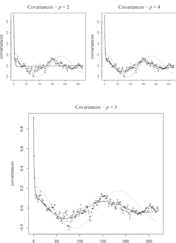
Example 2. The processx=OU_{(0.04,0.21,1.87)}is analysed as in Example 1. The result-ing estimators are ˇβββT = (−2.0611,−0.7459,−0.0553),T =270, ˇκκκ= (1.6224, 0.3378,

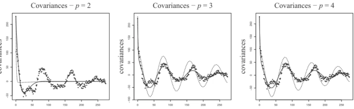
0 50 100 150 200 250 −0.2 0.0 0.2 0.4 0. 6 0. 8 Covariances −p= 2 Covariances −p=4 Covariances −p=3 covariances 0 50 100 150 200 250 −0.2 0. 0 0 .2 0.4 0 .6 0.8 covariances 0 50 100 150 200 250 −0.2 0.0 0 .2 0.4 0.6 0. 8 covariances

Figure 3: Empirical covariances (◦) and covariances of the MC (—) and ML (- - -) fitted OU models, for p=2,p=4and p=3, the actual value of the parameter, corresponding to Example 3. The covariances of OUκκκare indicated with a dotted line.

The associated ARMA(3,2) model is

(1−1.9255B+1.05185B2−0.1200B3)x= (0.4831−0.9044B+0.4230B2)ǫ.

Example 3. The parameterκκκ = (0.83,0.0041,0.0009) used in the simulation of the OU processxtreated in the present example is approximately equal to the parameter ˆκκκ obtained by ML estimation with p=3 for Series A in Section 6.5.1. A graphical pre-sentation of the estimated covariances is given in Figure 3. The associated ARMA(3,2) model is

(1−2.4311B+1.8649B2−0.4339B3)x= (0.6973−1.3935B+0.6962B2)ǫ

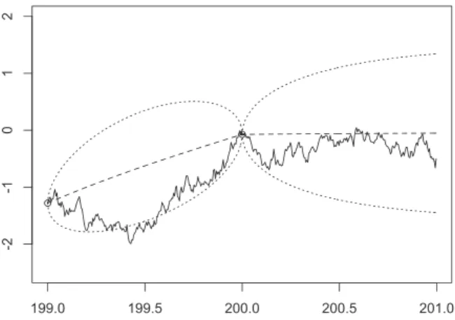
The description of the performance of the model is complemented by comparing in Figure 4 the simulated values of the process in 400 equally spaced points filling the interval (199,201) with the predicted values for the same interval, based on the OU(3) model and the assumed observed data x(0),x(2),x(3), . . .,x(200). Also a confidence band limited by the predicted values plus and minus twice their standard deviation (2-st.-dev. confidence band) is included in the graph, in order to describe the precision of the predicted values.

199.0 199.5 200.0 200.5 201.0 -2 -1 0 1 2

Figure 4: Estimated interpolation and prediction of x(t)for199<t<200and200<t<201, respectively (- - -), 2-st.-dev. confidence bands based on(x(i))i=0,1,...,200(· · ·), and a refinement of the simulation of x(t)

on199<t<200.

6.5. Applications to real data

In this section we present experimental results on two real data sets. We fit OU(p)

processes for small values of pand also some ARMA processes. In each case we have observed that we can find an adequate value ofpfor which the empirical covariances are well approximated by the covariances of the adjusted OU(p)model. This is not the case

for the ARMA models adjusted by maximum likelihood, in all examples. We present a detailed comparison of both methodologies for the first example.

The first data set is taken from Box, Jenkins, and Reinsel (1994), and correspond to equally spaced observations of continuous-time processes that might be assumed to be stationary. The second one is a series obtained by choosing one in every 100 terms of a high frequency recording of oxygen saturation in blood of a newborn child. The data were obtained by a team of researchers of Pereira Rossell Children Hospital in Montev-ideo, Uruguay, integrated by L. Chiapella, A. Criado and C. Scavone. Their permission to analyse the data is gratefully acknowledged by the authors.

6.5.1. Box, Jenkins and Reinsel “Series A”

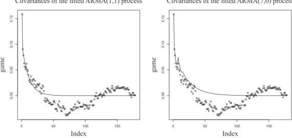
The Series A is a record ofn=197 chemical process concentration readings, taken every two hours, introduced with that name and analysed in (Box, Jenkins, and Reinsel, 1994, Ch. 4)1_{. Box et al. suggest an ARMA(1,1) as a model for this data, and subsets} of AR(7) are proposed in (Cleveland, 1971) and (McLeod and Zhang, 2006). Figure 5 shows that these models fit fairly well the autocovariances for small lags, but fail to capture the structure of autocorrelations for large lags present in the series. On the other hand, the approximations obtained with the OU(p) processes, for p=3,4 reflect both the short and long dependences, as shown in Figure 6.

0 50 100 150

0.00

0.05

0.10

0.15

Covariances of thefitted ARMA(1,1) process

Index gam e 0 50 100 150 0.00 0.05 0.10 0.15

Covariances of thefitted ARMA(7,0) process

Index

game

Figure 5: Empirical covariances (◦) and covariances of the ML (—) fitted models ARMA(1,1) and AR(7) for Series A.

0 50 100 150 0.00 0.05 0.10 0.15 Covariances −p= 3 Covariances −p=4 covariances 0 50 100 150 0.00 0.05 0.10 0.15 covari ances

Figure 6: Empirical covariances (◦) and covariances of the MC (—) and ML (- - -) fitted OU(p) models, for p=3,4corresponding to Series A.

It is interesting to consider jointly the ARMA(3,2) model (31) fitted to the origi-nal data by maximum likelihood (computed also with theR functionarima) and the ARMA(3,2) model (32) obtained by the procedure described in Section 5, correspond-ing to the OU(3) process also fitted to the data by maximum likelihood. The estimated parameters of this OU process are

ˆ κ κ

κ= (0.8293,0.0018+0.0330i,0.0018−0.0330i) and ˆc=0.4401

and the ARMA(3,2) processes are respectively

(1−0.7945B−0.3145B2+0.1553B3)x=0.3101(1−0.4269B−0.2959B2)ǫ (31)

and

(1−2.4316B+1.8670B2−0.4348B3)x=0.4401(1−1.9675B+0.9685B2)ǫ. (32)

The autocorrelations of both ARMA models, shown in Figure 7, together with the empirical correlations of the series were computed by means of theRfunctionARMAacf, although the ones corresponding to (32) could have been obtained as the restrictions to integer lags of the covariance function for continuous-time described in Section 3.2. It is worth to notice that the autocorrelations of (31) do not approach the empirical correlations, indicated by circles, as much as the correlations of (32). The logarithms of the likelihoods of (31) and (32) areℓ′=−49.23, andℓ′′=−50.95, respectively. But since the number of parameters of the second model (which is four) is smaller than the number of parameters of the complete family of ARMA(3,2) processes (six), the Akaike

0 50 100 150 −0.2 0.0 0.2 0.4 0.6 0 .8 1.0 lag correlations ARMA(3,2) OU(3)

Figure 7: Empirical correlations (◦) of Series A, and autocorrelations of models (31) and (32) fitted by maximum likelihood from the family of all ARMA(3,2) and the restricted family of ARMA(3,2) derived from OU(3). 190 192 194 196 198 200 17.0 17.5 18.0 ( − 7):( + 4)n n x

information criterion (AIC) of the parsimonious OU model is 8−2ℓ′′_{=109.90, slightly} better than the AIC of the unrestricted ARMA model, equal to 12−2ℓ′_=110.46.

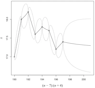
Finally we show in Figure 8 the predicted values of the continuous parameter process

x(t), fort betweenn−7 andn+4 (190-201), obtained as the best linear predictions based on the last 90 observed values, and on the correlations given by the fitted OU(3) model. The upper and lower lines are two standard deviation confidence limits for each value of the process.

6.5.2. Oxygen saturation in blood

The oxygen saturation in blood of a newborn child has been monitored during 17 hours, and measures taken every two seconds. We assume that a seriesx0,x1, . . . ,x304of mea-sures taken at intervals of 200 seconds is observed, and fit OU processes of orders

p=2,3,4 to that series. 0 50 100 150 200 250 −50 0 50 100 1 5 0 200

Covariances −p= 2 Covariances −p=3 Covariances −p=4

covariances 0 50 100 150 200 250 −100 −5 0 0 50 100 150 200 cova riances ri 0 50 100 150 200 250 −5 0 0 5 0 100 150 200 covari ances

Figure 9: Empirical covariances (◦) and covariances of the MC (—) and ML (- - -) fitted OU(p) models for p=2,3,4corresponding to the series of oxygen saturation in blood.

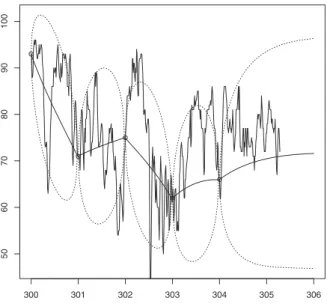
Again the empirical covariances of the series and the covariances of the fitted OU(p) models for p=2,3,4 are plotted (see Figure 9) and the estimated interpolation and extrapolation are shown in Figure 10. In the present case, the actual values of the series for integer multiples of 1/100 of the unit measure of 200 seconds are known, and plotted in the same figure.

6.6. Estimating the shape of the L ´evy noise

There are various methods proposed in the literature to estimate the parameters of L´evy driven Ornstein–Uhlenbeck processes; in particular, the L´evy-Khinchin triplet com-prised of two real numbers and a measure. For example, Valdivieso, Schoutens, and Tuerlinckx (2009) propose a maximum likelihood estimation methodology based on the inversion of the characteristic function of the L´evy process and the use of the discrete fast Fourier transform. Jongbloed, van der Meulen, and van der Vaart (2005) propose a nonparametric estimation based on a preliminary estimator of the characteristic func-tion. Both methods require a large amount of information and intensive computafunc-tion.

300 301 302 303 304 305 306 50 60 70 80 90 100

Figure 10: Partial graph showing the five last values of the series of O2 saturation in blood at integer

multiples of the 200 seconds unit of time (◦), interpolated and extrapolated predictions (—), 2-st.-dev. confidence bands (· · ·), and actual values of the series.

We propose a naive method of estimating the parameters of the L´evy driven Ornstein– Uhlenbeck process that works in general situations when the maximum likelihood func-tion is not known or difficult to approximate. These estimators are easy to compute, but also require a large amount of data to attain high accuracy.

Our method of estimation resembles the methods described in (Yu, 2004) consist-ing on matchconsist-ing the characteristic function derived from the model and the empirical characteristic function derived from the data.

Given a L´evy processΛ(t), the characteristic function ofΛ(t)is E eiuΛ(t)_{= (E e}iuΛ(1)₎t_,

and is usually written as E eiuΛ(1)=eψΛ(iu)_{. The functionψ}

Λ(iu) =log E eiuΛ(1)is called

characteristic exponentand has the form

ψΛ(iu) =aiu− σ2 2 u 2₊Z |x|<1 (eiux−1−iux)dν(x) + Z |x|≥1 (eiux−1)dν(x) whereν({0}) =0, R |x|<1x2dν(x)<∞, R

|x|≥1dν(x)<∞. The L´evy-Khinchin triplet is

(σ2_{,a, ν).}

Assume that the admissible exponents belong to a parametric classΨ={ψθ:θ∈Θ}

whereΘ⊂Rd_{, and obtain the value ofθfor which a chosen quadratic distance between}

the exponential ofψθ(iu) and the empirical characteristic function of the residuals is

In order to ease notation, let us consider the case of an OU(p)model with parameter κ

κκof pairwise different components; eitherκκκ is known or it is estimated by maximum likelihood or matching correlation methods. The innovation in each componentξj is

ηj(t) =

Z t

t−1

e−κj(t−s)_dΛ(s),

so that the innovation ofxκis

η(t) = Z t t−1 g(t−s)dΛ(s) where g(t) = p X j=1 Kje−κjt.

Hence, if we denoteη:=η(1), we have

η∼ Z 1 0 g(1−s)dΛ(s)∼ Z 1 0 g(s)dΛ(s)

and its characteristic exponent is therefore

ψη(iu) =log E eiuη =log E eiu R1 0g(s)dΛ(s)₌ Z 1 0 ψΛ(iug(s))ds

Example 4. Consider the estimation of a noise sum of a Poisson process plus a

Gaus-sian term. Let us assume that the noise is given by

Λ(t) =σW(t) +a(N(t)−λt)

whereW is a standard Wiener process andNis a Poisson process with intensityλ. The family of possible noises depends on the three parameters (σ, λ,a). In this case, the characteristic exponent has a simple form:

ψΛ(1)(iu) =− σ2_u2 2 +λ(e iua_−iua−1), hence ψη(iu) = Z 1 0 −σ 2_u2_g2_(s) 2 +λ(e iug(s)a −iug(s)a−1) ds Defininggh= R1 0 g h_{(s)ds, we have} ψη(iu) =− σ2_u2_g 2 2 +λ −u 2_g 2a2 2 −i u3g3a3 6 + u4g4a4 24 +. . .

Then we propose to estimate the parameters by equating the coefficients ofu2,u3,u4

inψη(iu) with the corresponding ones in the logarithm of the empirical characteristic

function of the residuals.

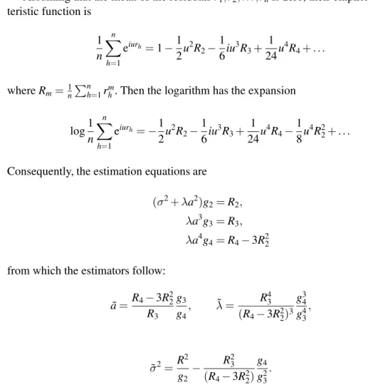
Assuming that the mean of the residualsr1,r2, . . . ,rnis zero, their empirical

charac-teristic function is 1 n n X h=1 eiurh₌₁₋1 2u 2_R 2− 1 6iu 3_R 3+ 1 24u 4_R 4+. . .

whereRm=1_nPnh=1rhm. Then the logarithm has the expansion

log1 n n X h=1 eiurh₌₋1 2u 2_R 2− 1 6iu 3_R 3+ 1 24u 4_R 4− 1 8u 4_R2 2+. . .

Consequently, the estimation equations are

(σ2_+λa2_)g 2=R2, λa3g3=R3, λa4g4=R4−3R22

from which the estimators follow:

˜ a=R4−3R 2 2 R3 g3 g4 , λ˜ = R 4 3 (R4−3R22)3 g3₄ g4 3 , ˜ σ2=R 2 g2 − R 2 3 (R4−3R22) g4 g2 3 .

Figure 11 shows the empirical c.d.f. of 90 estimators of the parameters obtained from simulated series of 200 terms. The residuals were obtained by applying a Kalman filter to the space state formulation, starting from the actual value ofκκκused at the simulation (-·-), that in practical situations is unknown, and from matching correlations estimation (– –) and by maximum likelihood estimation (–·–).

The estimators are not sharp at all, but the ones obtained by the same procedure applied directly on the unfiltered noiseΛ(– –) are equally rough. Larger series (of size 10000 and 1000000) produce sharper estimates, also shown in the figures by dotted lines.

c.d.f. of 90 estimators ofσ c.d.f. of 90 estimators ofλ c.d.f. of 90 estimators of c

Figure 11: Estimation of the parameters of the noise (σ–left panel–, λ–center–, a –right–) from 90 replications of{xκκκ(t):t=0,1, . . . ,200},κκκ= (0.01±0.1i,0.2), driven byΛ(t) =0.1W(t) +N0.3(t)−0.3t. Normality is rejected in all cases.

7. Conclusions

We have proposed a family of continuous-time stationary processes, based on p itera-tions of the linear operator that maps a second order L´evy process onto an Ornstein-Uhlenbeck process. These operators have some nice properties, such as being commu-tative, and theirp-compositions decompose as a linear combination of simple operators of the same kind. We remark that this result, stated in Theorem 1, is independent of the process onto which the operatorsOU_{κκκ act on. We have reduced the present scope of} the applications envisaged by applying the operators only to L´evy processes, but other choices deserve consideration, for example, the results of applying the same operators to fractional Brownian motions.

An OU(p)process depends onp+1 parameters that can be easily estimated by either maximum likelihood (ML) or matching correlations (MC) procedures. MC estimators provide a fair estimation of the covariances of the data, even if the model is not well specified. When sampled on equally spaced instants, the OU(p)family can be written as a discrete time state-space model; i.e., a VARMA model in a space of dimensionp. As a consequence, the families of OU(p)models are a parsimonious subfamily of the ARMA(p,p−1) processes in the Gaussian case. Furthermore, the coefficients of the ARMA can be deduced from those of the corresponding OU(p). We have shown exam-ples for which the ML-estimated OU model is able to capture features of the empirical autocorrelations at large lags that the ML-estimated ARMA model does not (see for in-stance Figure 7). This leads to recommend the inclusion of OU models as candidates to represent stationary series, either in discrete time or continuous-time.

References

Barndorff-Nielsen, O.E. (2001). Superposition of Ornstein-Uhlenbeck type processes.Theory of Probabil-ity and Its Applications, 45, 175–194.

Bergstrom, A.R. (1984). Continuous time stochastic models and issues of aggregation over time.Handbook of Econometrics, II, 1145–1212.

Bergstrom, A.R. (1996). Survey of continuous-time econometrics. InDynamic Disequilibrium Modeling: Theory and Applications: Proceedings of the Ninth International Symposium in Economic Theory and Econometrics, volume 9, page 1. Cambridge University Press.

Box, G.E.P. Jenkins, G.M. and Reinsel, G.C. (1994).Time Series Analysis, Forecasting and Control. Pren-tice Hall.

Brockwell, P.J. (2004). Representations of continuous-time ARMA processes.Journal of Applied Proba-bility, 41, 375–382.

Brockwell, P.J. (2009). L´evy–driven continuous–time ARMA processes. InHandbook of Financial Time Series, pages 457–480. Springer.

Cleveland, W.S. (1971). The inverse autocorrelations of a time series and their applications.Technometrics, 14, 277–298.

Doob, J.L. (1944). The elementary Gaussian processes.Annals of Mathematical Statistics, 15, 229–282. Durbin, J. (1961). Efficient fitting of linear models for continuous stationary time-series from discrete data.

Bulletin of the International Statistical Institute, 38, 273–282.

Durbin, J. and Koopman, S.J. (2001). Time Series Analysis by State Space Methods. Oxford University Press.

Eliazar, I. and Klafter, J. (2009). From Ornstein-Uhlenbeck dynamics to long-memory processes and Frac-tional Brownian motion.Physical Review E, 79, 021115.

Granger, C.W.J. (1980). Long memory relationships and the aggregation of dynamic models.Journal of Econometrics, 14, 227–238.

Granger, C.W.J. and Morris, M.J. (1976). Time series modelling and interpretation.Journal of the Royal Statistical Society. Series A, 139, 246–257.

Jongbloed, G., van der Meulen, F.H. and van der Vaart, A.W. (2005). Nonparametric inference for L´evy-driven Ornstein-Uhlenbeck processes.Bernoulli, 11, 759–791.

L¨utkepohl, H. (2005).New Introduction to Multiple Time Series Analysis. Springer Science & Business Media.

McLeod, A.I. and Zhang, Y. (2006). Partial autocorrelation parameterization for subset autoregression. Jour-nal of Time Series AJour-nalysis, 27, 599–612.

Nieto, B., Orbe, S. and Zarraga, A. (2014). Time-Varying Market Beta: Does the estimation methodology matter?SORT, 31, 13–42.

R Core Team. (2015).R: A Language and Environment for Statistical Computing. Technical report, R Foun-dation for Statistical Computing, Vienna, Austria.

Sato, K.-I. (1999).L´evy Processes and Infinitely Divisible Distribution, volume 68 ofCambridge Studies in Advance Mathematics. Cambridge University Press.

Thornton, M.A. and Chambers, M.J. (2013). Continuous-time autoregressive moving average processes in discrete time: representation and embeddability.Journal of Time Series Analysis, 34, 552–561. Uhlenbeck, G.E. and Ornstein, L.S. (1930). On the theory of the Brownian motion.Physical Review, 36,

823–841.

Valdivieso, L., Schoutens, W. and Tuerlinckx, F. (2009). Maximum likelihood estimation in processes of Ornstein-Uhlenbeck type.Statistical Inference for Stochastic Processes, 12, 1–19.

Yu, J. (2004). Empirical characteristic function estimation and its applications.Econometric Reviews, 23, 93–123.

Appendix A: Proofs of Theorem 1 and its corollaries

Parts(i)and(iii)are obtained by direct computation of the integrals,(ii)follows from

(i)by finite induction, as well as(iv)from(iii).

From the continuity of the integrals with respect to the parameterκ, the powerOUp_κ satisfies OU_κp_=lim δ↓0 p

∏

On the other hand, by(i),

q

∏

∏

∏

For theh-th term in the right-hand side of (34), we compute

lim δδδ↓0 p_h X j=1 K_h′′_,j(δδδ,κκκ)OU_κ h+jδh=lim_δδδ ↓0 p_h X j=1 K_h′′′_,j(δδδ,κκκ)K′_j(δh, κh,ph)OUκh+jδh =lim δδδ↓0 p_h X j=1 (Kh′′′,j(δδδ,κκκ)−Kh(κκκ))K′j(δh, κh,ph)OUκ_h+jδ_h + Kh(κκκ)lim δδδ↓0 p_h X j=1 K′j(δh, κh,ph)OUκ_h+jδ_h=Kh(κκκ)OUκphh

by Equation (33) since, in addition, each term in the first sum tends to zero. This ends the verification of(v).

Corollary 1 is an immediate consequence of(iv)and(v), and Corollary 2 follows by applying(i)to compute OU_λ+iµOU_λ−iµ=λ+iµ 2iµ OUλ+iµ− λ−iµ 2iµ OUλ−iµ = Z t −∞e −λ(t−s)hλ+iµ 2iµ (cos(µ(t−s)) +isin(µ(t−s))) −λ₂−_iµiµ(cos(µ(t−s))−isin(µ(t−s)))idΛ(s) = Z t −∞e −λ(t−s)_{(cos(µ(t−s)) +}λ µsin(µ(t−s)))dΛ(s).

Appendix B: Derivation of a state-space model

The form of equations (22) for a state-space representation of the OU(p)process in the general case can be derived by considering three special cases:

1. When the components ofκκκare all different. This case is treated in Section 4. 2. When the components ofκκκ are all equal. Letκdenote the common value of the

components ofκκκ. The state of the system is described by the vector ξξξκ,p= (ξκ(0), ξκ(1), . . . , ξκ(p−1)) T , with componentsξ_κ(h)(t) = Z t −∞e −κ(t−s)(−κ(t−s))h h! dΛ(s). Each of these terms can be written as the sum

ξ_κ(h)(t) =e−κ Z t−1 −∞ e −κ(t−1−s)(−κ(t−1−s+1))h h! dΛ(s) +ηκ,h(t) (35) whereηκ,h(t) = Z t t−1 e−κ(t−s)(−κ(t−s)) h h! dΛ(s). The first term in the right-hand side of (35) is equal to

e−κ h X j=0 (−κ)h−j (h−j)! Z t−1 −∞ e−κ(t−1−s)(−κ(t−1−s)) j j! dΛ(s) =e−κ h X j=0 (−κ)h−j (h−j)!ξ (j) κ (t−1)

and therefore, by introducing the matrix Aκ,p=e−κ               1 0 0 . . . 0 0 (−κ) 1! 1 0 . . . 0 0 (−κ)2 2! (−κ) 1! 1 . . . 0 0 .. . ... ... . .. ... ... (−κ)p−2 (p−2)! (−κ)p−3 (p−3)! (−κ)p−4 (p−4)! . . . 1 0 (−κ)p−1 (p−1)! (−κ)p−2 (p−2)! (−κ)p−3 (p−3)! . . . (−κ) 1! 1               we may write ξξξκ,p(t) =Aκ,pξξξκ,p(t−1) +ηηηκ,p

where ηηηκ,p(t) = (ηκ,0(t), ηκ,1(t), . . . , ηκ,p−1(t))T is a vector of centered inno-vations (independent of theσ-algebra generated by{Λ(s):s≤t−1}) with covari-ance matrixBκ,κ,pobtained withκ1=κ2andp1=p2from the genera