Estimating standard errors for importance sampling estimators with multiple Markov chains

Statistics Preprints Statistics

6-25-2015

Estimating standard errors for importance sampling

estimators with multiple Markov chains

Vivekananda Roy

Iowa State University, [email protected]

Aixin Tan

James M. Flegal

University of California, Riverside

Follow this and additional works at:http://lib.dr.iastate.edu/stat_las_preprints Part of theStatistics and Probability Commons

This Article is brought to you for free and open access by the Statistics at Iowa State University Digital Repository. It has been accepted for inclusion in Statistics Preprints by an authorized administrator of Iowa State University Digital Repository. For more information, please contact

[email protected].

Recommended Citation

Roy, Vivekananda; Tan, Aixin; and Flegal, James M., "Estimating standard errors for importance sampling estimators with multiple Markov chains" (2015).Statistics Preprints. 34.

Estimating standard errors for importance sampling estimators with

multiple Markov chains

Abstract

The naive importance sampling estimator based on the samples from a single importance density can be extremely numerically unstable. We consider multiple distributions importance sampling estimators where samples from more than one probability distributions are combined to consistently estimate means with respect to given target distributions. These generalized importance sampling estimators provide more stable estimators than the naive importance sampling estimators. Importance sampling estimators can also be used in the Markov chain Monte Carlo (MCMC) context, that is, where iid samples are replaced with positive Harris Markov chains with invariant importance distributions. If these Markov chains converge to their respective target distributions at a geometric rate, then under two finite moment conditions a central limit theorem (CLT) holds for the importance sampling estimators. In order to calculate valid asymptotic standard errors, it is required to consistently estimate the asymptotic variance in the CLT. Recently Tan and Doss and Hobert (2015) developed an approach based on regenerative simulation for obtaining consistent estimators of the asymptotic variance. It is well-known that in practice it is often difficult to construct a useful

minorization condition that is required in Tan and Doss and Hobert ’s (2015) regenerative simulation method. We provide an alternative estimator for these standard errors based on the easy to implement batch means methods. The multi-chain importance sampling estimators depend on Geyer’s (1994) reverse logistic estimator (of ratios of normalizing constants) which has wide applications, in its own right, in both frequentist and Bayesian inference. We also provide batch means estimator for calculating asymptotically valid standard errors of Geyer’s (1994) reverse logistic estimator. We illustrate the method with an application in Bayesian variable selection in linear regression. In particular, the multi-chain importance sampling estimator is used to perform empirical Bayes variable selection and the batch means estimator is used to obtain standard errors in the large p situation where regenerative method is not applicable.

Keywords

Bayes factors, Geometric ergodicity, importance sampling, Markov chain Monte Carlo, ratios of normalizing constants, standard errors

Disciplines

Statistics and Probability

Estimating standard errors for importance sampling

estimators with multiple Markov chains

Vivekananda Roy

, Aixin Tan

, and James M. Flegal

1

_{Department of Statistics, Iowa State University}

2

_{Department of Statistics and Actuarial Science, University of Iowa}

_{Department of Statistics, University of California, Riverside}

June 25, 2015

Abstract

The naive importance sampling estimator based on the samples from a single importance density can be extremely numerically unstable. We consider multiple distributions importance sampling es-timators where samples from more than one probability distributions are combined to consistently estimate means with respect to given target distributions. These generalized importance sampling estimators provide more stable estimators than the naive importance sampling estimators. Impor-tance sampling estimators can also be used in the Markov chain Monte Carlo (MCMC) context, that is, where iid samples are replaced with positive Harris Markov chains with invariant importance distributions. If these Markov chains converge to their respective target distributions at a geometric rate, then under two finite moment conditions a central limit theorem (CLT) holds for the impor-tance sampling estimators. In order to calculate valid asymptotic standard errors, it is required to consistently estimate the asymptotic variance in the CLT. Recently Tan and Doss and Hobert (2015) developed an approach based on regenerative simulation for obtaining consistent estimators of the asymptotic variance. It is well-known that in practice it is often difficult to construct a useful mi-norization condition that is required in Tan and Doss and Hobert ’s (2015) regenerative simulation method. We provide an alternative estimator for these standard errors based on the easy to imple-ment batch means methods. The multi-chain importance sampling estimators depend on Geyer’s (1994) reverse logistic estimator (of ratios of normalizing constants) which has wide applications, in its own right, in both frequentist and Bayesian inference. We also provide batch means estimator for calculating asymptotically valid standard errors of Geyer’s (1994) reverse logistic estimator. We illustrate the method with an application in Bayesian variable selection in linear regression. In par-ticular, the multi-chain importance sampling estimator is used to perform empirical Bayes variable selection and the batch means estimator is used to obtain standard errors in the large p situation where regenerative method is not applicable.

Key words and phrases: Bayes factors, Geometric ergodicity, importance sampling, Markov

1

Introduction

Letπ(x) =ν(x)/mbe a probability density function (pdf) onXwith respect to a measureµ(·).

Supposef :X→_Ris aπintegrable function and we want to estimateEπf :=

R

Xf(x)π(x)µ(dx).

Letπ1(x) = ν1(x)/m1 be another pdf onXsuch that{x : π(x) = 0} ⊂ {x : π1(x) = 0}. The

importance sampling estimator of Eπf based on iid samples X1, . . . , Xn from the importance

densityπ1is (see. e.g. Robert and Casella, 2004, chap. 3)

Pn i=1f(Xi)ν(Xi)/ν1(Xi) Pn i=1ν(Xi)/ν1(Xi) a.s. −→ Z X f(x)ν(x)/m ν1(x)/m1 π1(x)µ(dx) Z X ν(x)/m ν1(x)/m1 π1(x)µ(dx) = Eπf. (1.1) The above importance sampling estimator can also be used in the setting where the iid samples

{Xi}ni=1are substituted with realizations of a Markov chain, which is suitably irreducible and has

π1 as its stationary density (Hastings, 1970). Note that the estimator (1.1) requires the functions

ν, ν1 to be known. On the other hand, it does not depend on the normalizing constants m, m1

which are generally unknown in all practical examples.

In this article we consider situations where one wants to estimate Eπf for all π belonging

to a large collection Π. As mentioned below, this situation arises in different problems, both in

frequentist and Bayesian statistics. Although (1.1) provides consistent estimators of Eπf for all

π ∈ Πbased on asingleMarkov chain{Xn}n≥0with stationary densityπ1, (1.1) does not work

well unless ν1 puts appreciable mass under all π ∈ Π. Since otherwise the ratios ν(x)/ν1(x)

can be arbitrarily large for some sample values making the estimator (1.1) unstable. Generally,

there is not a single good importance sampling densityπ1 which is “close” to allπ ∈Π(see e.g.

Geyer, 1994). In this case a natural modification to the estimator (1.1) is to replace π1 in (1.1)

with a mixture ofkappropriately chosen “scattered” densities,π ≡Pk

i=1(ai/|a|)πi, wherea =

(a1, a2, . . . , ak)arek positive constants,|a| =

Pk

i=1ai, andπi(x) = νi(x)/mi, i = 1,2, . . . , k

arekdensities generally known upto normalizing constants. Supposen1, n2, . . . , nkare positive

integers,di =mi/m1, i= 2, . . . , k,withd1 ≡1, and the(k−1)dimensional vector

d= (m2/m1, . . . , mk/m1). (1.2)

Let {X_i(l)}nl

i=1 be iid sample from πl or a positive Harris Markov chain with invariant density

πl, l = 1,2, . . . , k. (See Meyn and Tweedie, 1993, chap. 10 for the definition of positive Harris

Markov chain.) Then asnl → ∞,for alll = 1,2, . . . , k, we have

ˆ η ≡ k X l=1 al nl nl X i=1 f(X_i(l))ν(X_i(l)) Pk s=1asνs(X (l) i )/ds !, _k X l=1 al nl nl X i=1 ν(X_i(l)) Pk s=1asνs(X (l) i )/ds ! (1.3) a.s. −→ k X l=1 al Z X f(x) ν(x) Pk s=1asνs(x)/ds πl(x)µ(dx) !, _k X l=1 al Z X ν(x) Pk s=1asνs(x)/ds πl(x)µ(dx) ! = Z X f(x)ν(x) ¯ π(x)π¯(x)µ(dx) Z X ν(x) ¯ π(x)π¯(x)µ(dx) =Eπf.

The above multiple samples based estimator has been discussed in the literature before. Vardi (1985), Gill, Vardi and Wellner (1988), Meng and Wong (1996), Kong et al. (2003), and Tan

(2004) consider estimation based on iid samples. The estimator is applicable to a much larger class of problems if Markov chain samples are allowed. Geyer (1994), Buta and Doss (2011) and Tan and Doss and Hobert (2015) study the case when only Markov chain samples are available from the importance densities and this is the setting we work in this paper. The multi-samples importance sampling estimator has many applications including Monte Carlo maximum likeli-hood estimation and Bayesian sensitivity analysis. In Section 4, we illustrate our methodology with an example of Bayesian sensitivity analysis.

As noted above, the estimatorηˆis consistent in both settings: iid samples as well as Markov

chain samples satisfying the usual regularity conditions. In practice, it is important to provide

valid standard errors associated with the Monte Carlo estimate η. Except for the recent work ofˆ

Tan and Doss and Hobert (2015), other authors largely avoid this very important issue. Tan and

Doss and Hobert (2015) provide a way of calculating standard errors of ηˆusing the method of

regeneration. The success of this method crucially depends on the construction of an appropriate

minorization condition. (See Mykland, Tierney and Yu (1995) for definition of minorization con-dition as well as the description of regeneration method.) As otherwise infrequent regenerations render this method practically useless. Successful applications of the regeneration method for calculating standard errors is problem specific and involves a great deal of trial and error (see e.g. Tan and Hobert (2009) and Roy and Hobert (2007)). In the present paper we provide

standard error estimators ofηˆusing easy-to-use batch means method. Our batch means estimator

is straightforward to implement and hence can be routinely applied in practice. In the process

we also establish central limit theorem (CLT) for ηˆgeneralizing some results in Buta and Doss

(2011).

The estimator ηˆin (1.3) depends on the vector d of ratios of normalizing constants which

are unknown in all practical applications. We consider the two-stage scheme studied in Buta and

Doss (2011) where first an estimate dˆof d is obtained using Geyer’s (1994) “reverse logistic

regression” method based on samples fromπl, l= 1,2, . . . , k, and then independently of the first

stage, new samples are used to estimate Eπf, π ∈ Π using the estimator ηˆ(dˆ) in (1.3) with dˆ

substituted ford. Buta and Doss (2011) showed that the asymptotic variance ofηˆ(dˆ)depends on

the asymptotic variance of d. Thus we study the CLT ofˆ dˆand provide a batch means estimator

of the asymptotic variance covariance matrix of d. Sinceˆ dˆinvolves multiple Markov chain

samples, here we need to use multivariate batch means estimator. Although, the form of the

asymptotic variance covariance matrix ofdˆis complicated, our consistent batch means estimator

is straightforward to code. Recently Doss and Tan (2014) provide an estimator of the variance

covariance matrix of dˆusing the method of regenerations, which, as mentioned before, may be

difficult to implement in practice.

The problem of estimatingd, the ratios of normalizing constants of unnormalized densities is

important in its own right and has many other applications both in frequentist and Bayesian infer-ence. When the samples are iid sequences, this is the biased sampling problem studied in Vardi (1985). Here are three instances where the problem of estimating ratios of normalizing constants arises naturally– calculation of likelihood ratios in missing data (or latent variable) models, cal-culation of mixture densities for use in the importance sampling as mentioned before and finally in calculation of Bayes factors which has many applications including the hyperparameter selec-tion problems in Bayesian analysis. We devote an entire secselec-tion (Secselec-tion 2) in this paper on this important problem of estimating ratios normalizing constants.

The rest of the paper is organized as follows. In Section 2, we consider the problem of

estimatingdusing Geyer’s (1994) reverse logistic regression method. In fact, we study the

gen-eral quasi-likelihood function proposed in Doss and Tan (2014). Unlike Geyer’s (1994) method, this extended quasi-likelihood function has the advantage of using user defined weights which is appropriate in situations where the multiple Markov chains have different mixing rates. We

establish the CLT for the resulting estimators of d and develop the batch means estimators of

their asymptotic covariance matrix. Section 3 contains the construction of CLT for η. In thisˆ

section, we also describe how valid standard errors ofηˆcan be obtained using the batch means

method. These easy to compute standard errors of η, developed in Section 3, has been recentlyˆ

used in Roy and Evangelou and Zhu (2014) for choosing the skeleton points in the importance sampling estimator (1.3). Section 4 contains a toy example showing the benefits of different weight functions. In Section 4 we also consider a standard linear regression model with moder-ately large number of variables and use the batch means estimator developed here for empirical Bayes variable selection. The proofs of the theorems are relegated to the appendix.

2

Estimating ratios of normalizing constants in the Markov

chain setting

In this section we consider the problem of estimating ratios of normalizing constants. In partic-ular, we havek densitiesπl = νl/ml, l = 1, . . . , k with respect to the measure µ, where theνl’s

are known functions and the ml’s are unknown constants. For eachl we have a positive Harris

Markov chain Φl = {X

(l)

1 , . . . , X

(l)

nl} with invariant density πl. Our objective is to estimate all

possible ratiosmi/mj, i6=jor, equivalently, the vectorddefined in (1.2).

Geyer (1994) proposed a method of estimatingd, which he called the “reverse logistic

regres-sion”. We now describe the method. Letn =P

nland setal =nl/nfor the moment. Define the

vectorζ by

ζl=−log(ml) + log(al), forl = 1, . . . , k, (2.1)

and let pl(x,ζ) = νl(x)eζl Pk s=1νs(x)eζs , forl= 1, . . . , k. (2.2)

Given that the valuexbelongs to the pooled sampleX_i(l), i= 1, . . . , nl, l = 1, . . . , k ,pl(x,ζ)

is the probability that x came from the lth sample. Of course, we know which distribution the

sample xcame from, but here we pretend that the only thing we know about xis its value and

estimateζby maximizing the log quasi-likelihood function

ln(ζ) = k X l=1 nl X i=1 log pl(Xi(l),ζ) (2.3)

with respect to ζ. Since ζ has a one-to-one correspondence withm = (m1, . . . , mk), by

es-timating ζ we can estimatem. As Geyer (1994) mentions, there is a non-identifiability issue

regarding ln(ζ): for any constant c ∈ R, ln(ζ) is same as ln(ζ +c1k) where 1k is the vector

m only up to an overall multiplicative constant, that is, we can estimate onlyd. Letζ₀ ∈ _Rk

be defined by [ζ₀]l = [ζ]l − Pk_s=1[ζ]s

/k, that is, ζ₀ is the true ζ normalized to add to zero.

Geyer (1994) proposed to estimate ζ₀ by ζ, the maximizer ofˆ ln subject to the linear constraint

ζ>1k = 0, and thus obtain an estimate ofd. The estimatordˆ(written explicitly in Section 2.1),

was introduced by Vardi (1985), and studied further by Gill et al. (1988), who proved that in the

iid setting, dˆis consistent and asymptotically normal, and established its optimality properties.

Later Geyer (1994) proved the consistency and asymptotic normality of dˆin the more general

setting where Φl,Φ2, . . . ,Φk are k Markov chains satisfying certain mixing conditions. In the

iid setting, Meng and Wong (1996), Kong et al. (2003), and Tan (2004) rederived the estimate, although using different computational schemes. None of the papers mentioned above discusses

how to consistently estimate the variance covariance matrix of dˆeven in the iid setting. Only

recently Doss and Tan (2014) address this important issue and, as mentioned in the introduction,

obtain a regeneration based estimator of the covariance matrix ofdˆin the Markov chain setting.

Doss and Tan (2014) mention that the optimality results of Gill et al. (1988) does not hold in the Markov chain case. In particular, when using Markov chain samples, the choice of the weights

aj = nj/n to the probability density νj/mj in the denominator of (2.2) is no more optimal

and should instead incorporate the “effective sample size” of different chains as they might have quite different rates of mixing. Doss and Tan (2014) introduce the following more general log quasi-likelihood function `n(ζ) = k X l=1 wl nl X i=1 log pl(X (l) i ,ζ) , (2.4)

where the vectorw∈_Rk_{is defined by}

wl =al

n

nl

, l= 1, . . . , k, (2.5)

for an arbitrary probability vector a. (Note the change of notation froml to`.) Clearly if al =

nl/n, thenwl = 1and (2.4) becomes (2.3). In the setting where the regeneration method can be

used, Doss and Tan (2014) proved the consistency (to the true valueζ₀) and asymptotic normality

of the constrained maximizer ζˆ(subject to the constraintζ>1k = 0) of (2.4). They also obtain

a regeneration based estimator of the asymptotic covariance matrix. They describe an empirical

method for choosing the optimal a based on minimizing the trace of the estimated covariance

matrix ofd. A crucial assumption in Doss and Tan’s (2014) results is the minorization condition,ˆ

that is, in order to implement their regenerative simulation method, it is needed to construct a

practically useful minorization condition for each of thekMarkov chainsΦl,Φ2, . . .Φk, which is

extremely difficult in practice. In the next section, without assuming such minorization condition,

we show that dˆis a consistent estimator ofd and also satisfies a CLT. We also provide a batch

means estimator of the covariance matrix ofd.ˆ

2.1

Central limit theorem and covariance estimation using batch means

In this section we discuss central limit theorems of the estimateζ, the maximizer of (2.4). Thisˆ

(1.2). We also construct consistent batch means estimator of the variance covariance matrix in the

CLT thus leading to asymptotically valid standard errors ford. Sinceˆ ζˆinvolves multiple Markov

chains, we need to use multivariate batch means estimator to calculate its standard errors. We assume thatn1, . . . , nk → ∞in such a way thatnl/n →sl∈(0,1), forl= 1, . . . , k. In order to

obtain the CLT result ford, we first establish a CLT forˆ ζˆ. Note that the functiong: _Rk _→

Rk−1

that mapsζ₀ intodis given by

g(ζ) =      eζ1−ζ2_a 2/a1 eζ1−ζ3_a 3/a1 .. . eζ1−ζk_a k/a1      , (2.6)

and its gradient atζ₀ (in terms ofd) is

D=        d2 d3 . . . dk −d2 0 . . . 0 0 −d3 . . . 0 .. . ... . .. ... 0 0 . . . −dk        . (2.7)

Sinced=g(ζ₀), and by definitiondˆ=g(ζˆ), we can use the CLT result ofζˆto get a CLT ford.ˆ

In order to state the CLT ofζˆ, we introduce the following notations.

Forr= 1,2, . . . , k, let

Y_i(r,l) =pr(Xi(l),ζ0)−Eπl pr(X,ζ0)

, i= 1, . . . , nl. (2.8)

The asymptotic variance covariance matrix in the CLT ofζ, involves twoˆ k×k matricesB

andΩ, which we now define. The matrixBis given by

Brr = k X j=1 ajEπj pr(X,ζ)[1−pr(X,ζ)] , r= 1, . . . , k, Brs =− k X j=1 ajEπj pr(X,ζ)ps(X,ζ) , r, s= 1, . . . , k, r6=s. (2.9)

LetΩbe thek×k matrix defined by

Ωrs = k X l=1 a2_l sl h Eπl{Y (r,l) 1 Y (s,l) 1 }+ ∞ X i=1 Eπl{Y (r,l) 1 Y (s,l) 1+i }+ ∞ X i=1 Eπl{Y (r,l) 1+i Y (s,l) 1 } i , r, s= 1, . . . , k. (2.10)

Remark1. Note that the right hand side of (2.10) involves terms of the formEπl{Y (r,l) 1 Y (s,l) 1+i }and Eπl{Y (r,l) 1+i Y (s,l)

1 }. For any fixedl, r, sand i, the two expectations are the same ifX

(l)

1 andX

(l) 1+i

are exchangeable, which happens if Φl = {X

(l)

i } nl

i=1 is a reversible chain. But in general cases

The matrixB will be estimated by its natural estimateBbdefined by b Brr = k X l=1 al 1 nl nl X i=1 pr(Xi(l),ζˆ) 1−pr(Xi(l),ζˆ) , r= 1, . . . , k, b Brs =− k X l=1 al 1 nl nl X i=1 pr(X (l) i ,ζˆ)ps(X (l) i ,ζˆ) , r, s= 1, . . . , k, r6=s. (2.11)

To obtain a batch means estimateΩb, suppose we simulate the Markov chainΦ_l forn_l = e_lb_l

iterations (henceel =enl andbl=bnl are functions ofnl) and define forr, l= 1, . . . , k

¯ Z_m(r,l) := 1 bl (m+1)bl X j=mbl+1 pr(X (l) j ,ζˆ) form = 0, . . . , el−1. Now set Z¯m(l) = ¯ Zm(1,l), . . . ,Z¯m(k,l) >

for m = 0, . . . , el − 1. Forl = 1,2, . . . , k, denote

¯ ¯ Z(l)= ¯ ¯ Z(1,l),Z¯¯(2,l), . . . ,Z¯¯(k,l) > whereZ¯¯(r,l)=Pnl i=1pr(X (l) i ,ζˆ)/nl. Let b Σ(l) = bl el−1 el−1 X m=0 h ¯ Z_m(l)−Z¯¯(l)i hZ¯_m(l)−Z¯¯(l)iT for l = 1,2, . . . , k. (2.12) Finally, let b Σ =           b Σ(1) b Σ(2) . . . . . . . . . ._.

0

0

and define the followingk×k2_matrix

An = − r n n1 a1Ik − r n n2 a2Ik . . . − r n nk akIk , (2.14)

whereIk denotes thek×kidentity matrix. Define

b

Ω = AnΣbA>_n. (2.15)

We are now ready to state the following theorem which describes the strong consistency, and

asymptotic normality of d. This theorem also provides consistent estimate of the asymptoticˆ

covariance matrix of dˆusing batch means method. As mentioned in Doss and Tan (2014), the

consistency of dˆholds under minimal assumptions on the Markov chainsΦ1, . . . ,Φk. In

partic-ular, ifΦ1, . . . ,Φk are positive Harris chains thendˆis a consistent estimator ofd. On the other

hand, CLTs and consistency of batch means estimator of asymptotic covariance require some mixing conditions on the Markov chains, and the most commonly used condition is that of

geo-metric ergodicity of the chains. For a square matrixC, letC†denote the Moore-Penrose inverse

Theorem 1 Suppose that for eachl = 1, . . . , k, the Markov chain{X₁(l), X₂(l), . . .}has invariant distributionπl.

(1) If the Markov chains Φ1, . . . ,Φk are positive Harris, the log quasi-likelihood function (2.4)

has a unique maximizer subject to the constraintζ>1k = 0. Letζˆdenote this maximizer, and

letdˆ=g(ζˆ). Thendˆ−→a.s. dasn1, . . . , nk→ ∞.

(2) If the Markov chainsΦ1, . . . ,Φkare geometrically ergodic, asn1, . . . , nk→ ∞,

√

n(dˆ−d)→ Nd (0, V) where V =D>B†ΩB†D. (2.16)

(3) Assume that the Markov chainsΦ1, . . . ,Φkare geometrically ergodic and for alll = 1,2, . . . , k,

bl = bnνlcwhere1 > ν > 0. LetDb be the matrixDin (2.7) withdˆin place ofd, and letBb

and Ωb be defined by (2.11) and (2.15), respectively. Then, Vb := Db>Bb†ΩbBb†Db is a strongly

consistent estimator ofV.

The proof of Theorem 1 is given in Appendix A.

Remark2. Since Theorem 1 does not require the chainsΦl, l = 1. . . , kto be stationary, there is

no need for burnin.

3

Importance sampling with multiple Markov chains

In this section we consider CLT and estimation of standard errors for the multi-chain importance

sampling estimatorηˆgiven in the Introduction.

From (1.3) we see thatηˆ≡ηˆ[f]_{(π;a,d) = ˆv}[f]_{(π, π}

1;a,d)/uˆ(π, π1;a,d), where ˆ u≡uˆ(π, π1;a,d) := k X l=1 al nl nl X i=1 u(X_i(l);a,d) and vˆ≡ˆv[f](π, π1;a,d) := k X l=1 al nl nl X i=1 v[f](X_i(l);a,d) (3.1) with u(x;a,d) := ν(x) Pk s=1asνs(x)/ds and v[f](x;a,d) := f(x)u(x;a,d). (3.2) Note that ˆ u−→a.s. k X l=1 alEπlu(X;a,d) = Z X Pk l=1alνl(x)/ml Pk s=1asνs(x)/(ms/m1) ν(x)µ(dx) = m m1 , (3.3)

as n1, . . . , nk → ∞. Thus uˆ itself is a useful quantity as it consistently estimates the ratios of

normalizing constants {u(π, π1) ≡ m/m1|π ∈ Π}. Unlike the estimator dˆin Section 2, the

above estimator uˆ in (3.1) does not require sample from each density π ∈ Π. Thus uˆ is well

suited for the situations where one wants to estimate the ratios u(π, π1)for a very large number

ofπ’s based on samples from a small number (k) of skeleton densities.

In the context of Bayesian analysis, letπ(x) = lik(x)p(x)/mbe the posterior density

case,u(π, π1)is the so-called Bayes factor between the two models. The Bayes factors are often

used in model selection. Recently, Roy and Evangelou and Zhu (2014) estimate link function and covariance function parameters in spatial generalized linear mixed models by calculating

ˆ

u corresponding to a large number (combination) of these parameter values and subsequently

choosing that value which maximizes the marginal likelihood function.

The estimatorsuˆ and vˆin (3.1) depend on d, which is generally unknown in practice. As

mentioned in the Introduction, here we consider a two-stage procedure for evaluating u. In theˆ

1st stage,dis estimated by its reverse logistic regression estimatordˆdescribed in Section 2 using

Markov chains Φ˜l ≡ {X˜il} Nl

i=1 with stationary densityπl, for l = 1, . . . , k. Note the change of

notation from Section 2 where we used nl’s to denote the length of the Markov chains. In order

to avoid introducing more notations and since estimatingdis not the primary goal of this section,

we useΦ˜l’s andNl’s to denote the stage 1 chains and their length respectively. Oncedˆis formed,

new MCMC samples Φl ≡ {Xil}

nl

i=1, l = 1. . . , k are obtained and u(π, π1)(Eπf) is estimated

using uˆ(π, π1;a,dˆ)(ηˆ[f](π;a,dˆ)) based on these 2nd stage samples. This two-stage method is

proposed in Buta and Doss (2011) who quantify its benefits over the single stage method where

the same MCMC samples are used to estimate both d andu(π, π1). In Section 3.1 we present

a CLT foruˆand construct batch means estimator of its asymptotic variance. Finally, we discuss

the estimation of standard errors ofηˆin Section 3.2.

3.1

Estimating a large number of ratios of normalizing constants

Before we state a CLT foruˆ(π, π1;a,dˆ), we define the following notations:

τ_l2(π;a,d) =Varπl(u(X (l) 1 ;a,d)) + 2 ∞ X g=1 Covπl(u(X (l) 1 ;a,d), u(X (l) 1+g;a,d)), (3.4) τ2_{(π;a,d) =} Pk l=1(a 2

l/sl)τl2(π;a,d), c(π;a,d) is a vector of length k − 1 with (j − 1)th

coordinate as [c(π;a,d)]j−1 = u(π, π1) d2 j Z X ajνj(x) Pk s=1asνs(x)/ds π(x)dx forj = 2, . . . , k, (3.5) ˆ

c(π;a,d)is a vector of lengthk−1with(j −1)th coordinate as

[ˆc(π;a,d)]j−1 ≡ k X l=1 1 nl nl X i=1 ajalν(X (l) i )νj(X (l) i ) (Pk s=1asνs(X (l) i )/ds)2d2j forj = 2, . . . , k, (3.6) and assumingnl =elml ˆ τ_l2(π;a,d) = bl el−1 el−1 X m=0 [¯um(a,d)−u¯¯(a,d)]2, (3.7)

whereu¯m(a,d)is the average of the(m+ 1)st block{u(X

(l)

mbl+1;a,d),· · · , u(X (l)

(m+1)bl;a,d)},

and u¯¯(a,d)is the overall average of {u(X₁(l);a,d),· · · , u(Xn(ll);a,d)}. Here, bl andel are the

block sizes and the number of blocks respectively. Finally letτˆ2(π;a,d) =Pk

l=1(a 2

Theorem 2 Suppose that for the stage 1 chains, conditions of Theorem 1 holds such thatN1/2_(dˆ−

d) → Nd (0, V)asN ≡ Pk

l=1Nl → ∞. Assume that the stage 2 Markov chainsΦ1, . . . ,Φk are

geometrically ergodic, and there exists >0such that

Eπl|u(X;a,d)|

2+ _<∞

for eachl = 1,· · ·, k. Suppose there existsq ∈[0,∞)such thatn/N → qwheren = Pk

l=1nl

is the total sample size for stage 2. In addition, letnl/n→slforl= 1,· · · , k.

(1) Then asn1, . . . , nk → ∞,

√

n(ˆu(π, π1;a,dˆ)−u(π, π1))

d

→N(0, qc(π;a,d)>V c(π;a,d) +τ2(π;a,d)). (3.8)

(2) Let Vb be the consistent estimator of V given in Theorem 1 (3). Assume that there exist

> 0, δ > 0such that Eπl|u(X;a,d)|

2+δ+ _{< ∞for all l = 1,2, . . . , k, b}

l = bnνlc where

1 > ν > 2/(2 + δ). Then qˆc(π;a,dˆ)>Vbcˆ(π;a,dˆ) + ˆτ2(π;a,dˆ)) is a strong consistent

estimator of the asymptotic variance in (3.8).

The proof of Theorem 2 is given in Appendix B.

Note that the asymptotic variance in (3.8) has two components. The second term is the

vari-ance ofuˆwhendis known. The 1st term is the increase in the variance ofuˆresulting from using

ˆ

dinstead of d. Since we are interested in estimatingu(π, π1)for a large number ofπ’s and for

every π the computational time needed to calculate uˆin (3.1) is linear in the total sample size

n, this can not be very large. If generating MCMC samples is not computationally demanding,

then long chains can be used in the 1st stage (that is, large Nl’s can be used) to obtain a precise

estimate ofd, thus greatly reducing the first term in the variance expression (3.8).

3.2

Estimation of expectations using multiple chain importance sampling

In this section we discuss the estimation of standard errors of the multi chain importance sampling estimatorηˆgiven in (1.3). Recall from (3.1) thatηˆ≡ηˆ[f]_{(π;a,d) = ˆv}[f]_{(π, π}

1;a,d)/uˆ(π, π1;a,d), where vˆ ≡ vˆ[f]_{(π, π} 1;a,d) := Pk l=1(al/nl) Pnl i=1v[f](X (l) i ;a,d) and uˆ ≡ uˆ(π, π1;a,d) := Pk l=1(al/nl) Pnl i=1u(X (l) i ;a,d).

In order to state a CLT forηˆwe define the following notations:

γ_l11 ≡γ_l11(π;a,d) =Varπl(v [f] (X₁(l);a,d)) + 2 ∞ X g=1 Covπl(v [f] (X₁(l);a,d), v[f](X₁₊(l)_g;a,d)), γ12_l ≡γ_l12(π;a,d) =γ_l21 ≡γ_l21(π;a,d) =Covπl(v [f]_(X(l) 1 ;a,d), u(X (l) 1 ;a,d)) + ∞ X g=1 [Covπl(v [f]_(X(l) 1 ;a,d), u(X (l) 1+g;a,d)) +Covπl(v [f]_(X(l) 1+g;a,d), u(X (l) 1 ;a,d))], γ_l22≡γ_l22(π;a,d) = Varπl(u(X (l) 1 ;a,d)) + 2 ∞ X g=1 Covπl(u(X (l) 1 ;a,d), u(X (l) 1+g;a,d)),

(Note that,γ22

l is same asτl2(π;a,d))defined in (3.4).) and

Γl(π;a,d) = γ11 γ12 γ21 γ22 ; Γ(π;a,d) = k X l=1 a2_l sl Γl(π;a,d). (3.9)

Since ηˆ has the form of a ratio, to establish a CLT for it, we apply the Delta method on the

functionh(x, y) =x/y, with∇h(x, y) = (1/y,−x/y2)0. Let

ρ(π;a,d) = ∇h(Eπf u(π, π1), u(π, π1))0Γ(π;a,d)∇h(Eπf u(π, π1), u(π, π1)), (3.10)

e(π;a,d)is a vector of lengthk−1with(j−1)th coordinate as

[e(π;a,d)]j−1 = aj d2 j Z X [f(x)−Eπf]νj(x) Pk s=1asνs(x)/ds π(x)dx, j = 2, . . . , k, (3.11)

andˆe(π;a,d)is a vector of lengthk−1with(j −1)th coordinate as

[ˆe(π;a,d)]j−1 ≡ Pk l=1 al nl Pnl i=1 ajf(Xi(l))ν(X (l) i )νj(X (l) i ) d2 j( Pk s=1asνs(Xi(l))/ds)2 Pk l=1 al nl Pnl i=1 ν(X_i(l)) Pk s=1asνs(Xi(l))/ds − [c(π;a,d)]j−1ηˆ [f]_(π;a,d) ˆ u(π, π1;a,d) , (3.12)

where[c(π;a,d)]j−1is defined in (3.6). We use the same two-stage procedure, as in Section 3.1,

for evaluatingη. Again assumingˆ nl =elml, let

b Γl(π;a,d)≡ bl el−1 el−1 X m=0 " ¯ v[mf] ¯ um − ¯ ¯ v[f] ¯ ¯ u #" ¯ vm ¯ um − ¯ ¯ v[f] ¯ ¯ u #> (3.13) = bl el−1   Pel−1 m=0 h ¯ vm[f]−v¯¯[f] i2 Pel−1 m=0 h ¯ v[mf]−¯¯v[f] i [¯um−u¯¯] Pel−1 m=0 h ¯ vm[f]−v¯¯[f] i [¯um−u¯¯] Pel−1 m=0[¯um−u¯¯] 2   (3.14) = ˆ γ11_{(π;a,d) ˆγ}12_(π;a,d) ˆ γ21(π;a,d) ˆγ22(π;a,d) ,say, (3.15)

where v¯m[f] is the average of the (m+ 1)st block{v[f](X_mb(l)_l+1;a,d),· · · , v[f](X₍(_ml)_+1)b

l;a,d)},

¯ ¯

v[f] is the overall average of {v[f](X₁(l);a,d),· · · , v[f](Xn(ll);a,d)}andu¯m ≡ u¯m(π,a,d),u¯¯ ≡

¯ ¯

u(π,a,d)defined in Section 3.1. Finally letΓ(b π;a,d) = Pk l=1(a 2 l/sl)bΓ_l(π;a,d), and ˆ ρ(π;a,dˆ) =∇h(ˆv[f](dˆ),uˆ(dˆ))0bΓ(π;a,dˆ)∇h(ˆv[f](dˆ),uˆ(dˆ)).

Theorem 3 Suppose that for the stage 1 chains, conditions of Theorem 1 holds such thatN1/2(dˆ−

d) → Nd (0, V)asN ≡ Pk

l=1Nl → ∞. Assume that the stage 2 Markov chainsΦ1, . . . ,Φk are

geometrically ergodic, and there exists >0such that

Eπl|u(X;a,d)|

2+

<∞ and Eπl|v

[f]

(X;a,d)|2+ <∞ (3.16)

for eachl = 1,· · ·, k. Suppose there existsq ∈[0,∞)such thatn/N → qwheren = Pk

l=1nl

(1) Then asn1, . . . , nk → ∞,

√

n(ˆη[f](π;a,dˆ)−Eπf)

d

→N(0, qe(π;a,d)>V e(π;a,d) +ρ(π;a,d)). (3.17)

(2) Let Vb be the consistent estimator of V given in Theorem 1 (3). Assume that there exists

> 0 such that (3.16) holds for all l = 1,2, . . . , k, bl = bnνlc where 1 > ν > 0. Then

qˆe(π;a,dˆ)>Vbˆe(π;a,dˆ) + ˆρ(π;a,dˆ))is a strong consistent estimator of the asymptotic

vari-ance in (3.17).

The proof of Theorem 3 is given in Appendix C.

Remark 3. Theorem 2 (1) and Theorem 3 (1) extend Buta and Doss’s (2011) Theorem 1 and

Theorem 3 respectively who consider the special case whenal=nl/n. Tan and Doss and Hobert

(2015) mention thatal = nl/n is not an optimal choice fora. This is why here we consider a

general arbitrary vectora.

Remark4. In the case whendis unknown, Tan and Doss and Hobert (2015) provide a

regener-ation based consistent estimator of the asymptotic variance of uˆandηˆin the special case when

a = (1,dˆ). With this particular choice, u(x;a,dˆ) and v[f]_{(x;a,dˆ) in (3.2) become free of dˆ}

leading to independence among certain quantities. As can be seen in the proofs of Theorem 2 in Appendix B and Theorem 3 in Appendix C, proving consistency of the batch means estimators

of the variances ofuˆandηˆin the general case requires careful, deep calculations.

Remark 5. As mentioned in Remark 4, Tan and Doss and Hobert (2015) provide regeneration

estimators for calculating standard errors ofuˆandηˆin the special case whena= (1,dˆ). We now

describe a trick that will essentially allow any choice ofafor Tan and Doss and Hobert ’s (2015)

regeneration estimator. In particular, set a = w∗(1,dˆ) for any user specified fixed vector w.

This general choice ofastill allow the expressions in (2.18) of Tan and Doss and Hobert (2015)

to be free ofd, thus leading to the independence of certain quantities required for their estimatorˆ

to work (details are given in the supplementary materials). This method was not mentioned in Tan and Doss and Hobert (2015).

4

Illustrations

In Section 4.1 through a toy example, we first discuss the different choices of weight functions and their effect on the estimates of expectations and ratios of normalizing constants. Next in Sec-tion 4.2, we use our batch means method for empirical Bayes variable selecSec-tion in the context of standard linear regression models with moderately large number of variables where regeneration based simulation is impractical.

4.1

Toy example

Lettr,µdenote the t-distribution with degree of freedom rand central parameterµ. We consider

a toy example whereπ1(·)andπ2(·)are the density functions fort5,µ1=1 andt5,µ2=0respectively.

For simplicity, let νi(·) = πi(·)for i = 1,2. Our plan is (1) to estimate the ratio between the

µ ∈ M} where M is a fine grid over [0,1], say M = {0, .01,· · ·, .99,1}. For each µ ∈ M,

we assume thatνµ(·) = πµ(·), and we want to learn the ratio between the normalizing constants

throughdµ :=

mµ

m1, as well as the expectation of each distribution inΠ,Et5,µX, written asEµX

for short. Clearly, we know the exact answer to all the questions above: d = dµ = 1 and

Et5,µX =µfor anyµ∈ M. Nevertheless, we follow the two-stage procedure from section 3 to

generate Markov chains fromπ1andπ2respectively, and build MCMC estimators as described in

Theorem 1, 2, and 3. The main goal is to check the performance of the batch means (BM) and the regeneration based simulation (RS) estimators for the asymptotic variance of these estimators.

We will draw iid samples fromπ1, and draw Markov chain samples fromπ2using the so called

“independent Metropolis Hastings (MH) algorithm” with proposal density t5,1. For i = 1,2,

we will draw Ni observations from πi in stage 1, andni observations from πi in stage 2. We

set N1 ≈ N2 and n1 ≈ n2, and further ask stage 2 sample sizes to be smaller than that of

stage 1, specifically, n1 = N1/10, due to reasons about computing cost explained right after

Theorem 2. We consider an increasing sequence of sample sizes, fromn1 = 103 to105, in order

to examine trace plots for the BM and the RS estimates of the asymptotic variances. Such two stage procedures are repeated 1000 times, so that empirical estimates of the asymptotic variances can be calculated and used to evaluate our estimators.

Note that, for estimators based on stage 1 samples, Theorem 1 allows any choice of weight,

a1_{. And for estimators based on stage 2 samples, Theorem 2 and 3 allow any choice of weight,a}2_,

in constructing BM estimators. As for RS estimators, similar Theorems hold and are described in Doss and Tan (2014); Tan and Doss and Hobert (2015). Recall from Remark 5 that we made an important generalization to existing theorems concerning RS estimators. That is, essentially any non-negative numerical vector can now be used as weight. We will discuss the choice of weights and their impact on the estimators in a separate section below. For now, we use the toy example to check the aforementioned Theorems, to see if both the BM estimator and the RS estimator are consistent, regardless of the weight chosen.

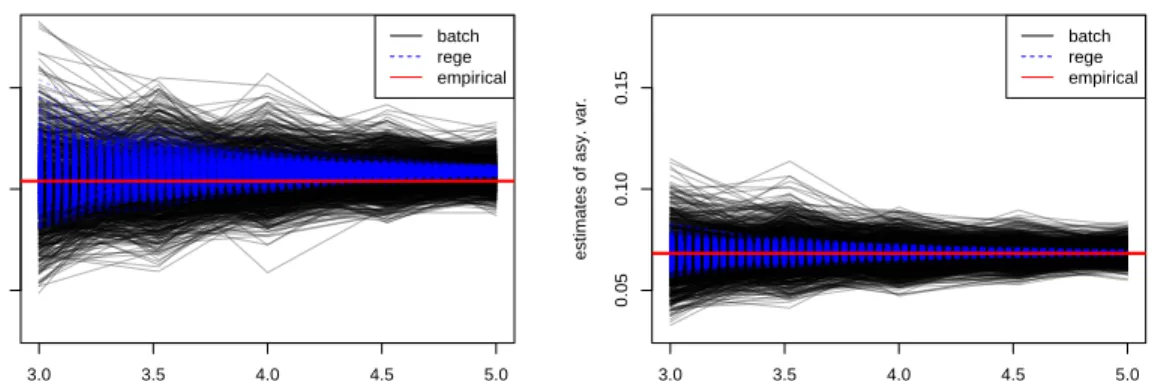
Figure 1 displays the BM and the RS estimates of dˆin stage 1, obtained from each of the

replications. They are evaluated at a sequence of sample sizes, from n1 = 103 to 105, and we

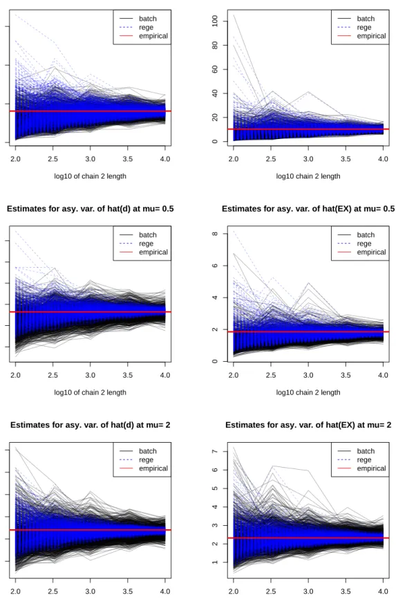
can see that both the BM and the RS estimates approach the empirical asymptotic variance as the sample size increases, suggesting their consistency. Also, as expected, the BM estimator are more variable than the RS estimates. Similarly, Figures 2 to 4 show convergence of the BM and the RS

estimators to the empirical asymptotic variance ofdˆµandEˆµ(X)respectively, in stage 2. (Small

deviations between the limit of the estimators and the empirical asymptotic variance are probably due to the fact that we do not know the true asymptotic variance, but are using an empirical estimate of it based on a finite sample size over a finite number of repetitions. Also, only plots

at selected values of µ∈M are shown due to space limit, but convergence of the estimators are

indeed observed in all the case we have inspected. )

Overall, the simulations study suggests that both the BM and the RS methods provide con-sistent estimators for the true asymptotic variance. Also, the RS estimators enjoy smaller mse in most cases. Nevertheless, when the number of regenerations is not great, BM estimators could be

the more stable estimator. For example, in the top left plot of Figure 2, at sample sizen2 = 1000,

in more than 5 out of the 1000 replications, RS estimators wildly over estimated the target. Fur-ther, in the cases where regeneration is “not viable”, i.e., where the number of regenerations is extremely small for any affordable sample size, BM would be the more stable estimator, or the

only reliable estimator between the two.

Choice of weights in stage 1

In practice, for stage 1, we recommend obtaining a close-to-optimal weight, a1opt_{, using a}

short pilot study. See Doss and Tan (2014) for details on how the pilot study can be done. The

right panel of Figure 1 displays empirical asymptotic variance of dˆover 1000 replications with

n1 = 105. For comparison, the left panel of Figure 1 presents such results based on the naive

choice of a1 _{= (.5, .5). The naive choice is determined by the relative sample sizes of the}

refer-ence chains, which is an asymptotically optimal choice had both chains been independent. But

in our example where chain 2 involves dependent samples, using a1opt results in dˆwith smaller

standard errors.

3.0 3.5 4.0 4.5 5.0

0.05

0.10

0.15

log10 of chain 1 length

estimates of asy. v ar . batch rege empirical 3.0 3.5 4.0 4.5 5.0 0.05 0.10 0.15

log10 of chain 1 length

estimates of asy. v ar . batch rege empirical

Figure 1: Estimates of the asymptotic variance ofdˆin stage 1.

Choice of weights in stage 2

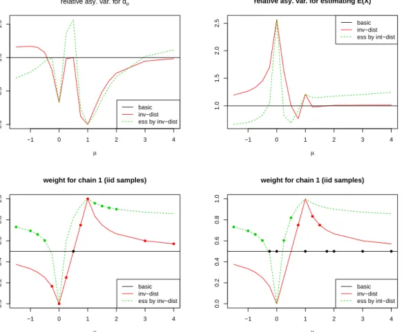
As for stage 2, where we have a sea of parameter values of interest, for eachµ ∈ M, there

would be a weighta2(µ)that is optimal for estimatingdµ, yet another weighta2(µ)that is optimal

for estimatingEt5,µX. Again, a pilot study can be used to find approximations for the2|M|sets

of optimal weights, or a selected subset of them scattered insideM. A less costly alternative is to

seta2(µ)to be inversely proportional to the deviation ofπµfrom thekreference points. Different

ways of defining deviation may be appropriate in different problems, here we simply measure the deviation betweent5,µandt5,µ0 by|µ−µ0|. Further adjustment ofa2(µ)are possible that assigns

the more efficient chains heavier weight. After all, we experiment with the following strategies for stage 2 estimates.

1. basic: a2 _{= (.5, .5)}

2. inv-dist: a2_(µ)∝( 1

|µ−µ1|, 1

3. ess by inv-dist: a2_(µ)∝(ess

1,ess2)∗(_|µ−1_µ 1|,

1

|µ−µ2|), where∗denotes point-wise product.

Not surprisingly, none of the three strategies is a clear winner, and their performances vary

greatly depending on the quantity being estimated (dµ or Eµ(X), or the expectation of other

functions), as well as on whether we are only interested in µ falling in between the reference

values µ1 = 1andµ2 = 0, or beyond. Still, we visualize the simulation results in Figure 5 and

summarize the situation briefly.

For estimatingdµ

1. Forµ∈(0,1), strategy 2 works the best.

2. Forµ= 0, strategy 2 and 3 work better than strategy 1. Indeed, both of them simply set their

stage 2 estimatesdˆ0 to be the stage 1 estimate,d. This would be a better choice than strategyˆ

1 because in a two-step procedure, stage 1 chains are often much longer than stage 2 chains,

and hencedˆis already a very accurate estimate ford0 =d.

3. Though not recommended, in case it is of interest to explore µ /∈ [0,1], strategy 2 and 3

generally leads to more stable estimates of dµ. However, all strategies lead to much larger

asymptotic variances than desired. Indeed, in case µ /∈ [0,1], it’s better to reconsider the

choice of reference chains to be drawn atµin its vicinity.

For estimatingEµ(X)

1. Forµ∈(0,1), strategy 2 works the best in general. Strategy 3 is very unstable.

2. For eitherµ= 0or1, strategy 2 and 3 are the same, and they only utilize the reference chain

fromµ. This was a wise choice for estimatingdµas explained above, but not so for any other

quantities of interest.

After all, strategies 2 and 3 have an advantage over using the naive weight when the

esti-mands are ratios between normalizing constants. However, when estimatingEµ(X), the situation

is more complicated. Our impression is that assigning any extreme weight will lead to high vari-ability in the estimator. So it is reasonable to simply use the naive weight, or use other strategies

that bound the weights from0and1.

5

Discussion

In this paper we consider two separate but related problems. The first problem is to estimate the

ratios of unknown normalizing constants given Markov chain samples from each of thek

proba-bility densities for some integerk larger than 1. The second problem is to estimate expectations

of a function with respect to a large number of probability distributions. The two problems are related in the sense that the multiple chains importance sampling estimators used for the latter uses the estimates derived for solving the first problem. The first situation also arises in a variety of contexts other than the multiple chain importance sampling estimators. In both situations, we consider estimators derived by methods involving flexible choice of weights and thus these es-timators are appropriate for Markov chains with different mixing behaviors. We establish CLTs

for these estimators and develop batch means methods for consistently estimating their standard errors. Although we compare batch means and regeneration based methods in this paper, spectral methods can also be used for variance estimation. Generally estimation by spectral methods is computationally more expensive (Doss and Tan, 2014, p. 703). Flegal and Jones (2010) com-pare the performance of confidence intervals produced by batch means, regeneration and spectral methods for the time average estimator, and they conclude that if tuning parameters are chosen appropriately, all these three methods perform equally well.

Appendices

A

Proof of Theorem 1

Proof. The proof of the consistency ofdˆfollows from Doss and Tan (2014) (section A.1) and is

omitted. Now onward, we use D&T to denote Doss and Tan (2014). Establishing a CLT for dˆ

is although analogous to section A.2 of D&T, there are some significant differences. Below we

establish the CLT fordˆand finally, we show thatVb is a consistent estimator ofV.

We begin by consideringn1/2_(ζˆ−ζ

0). As before, let∇represents the gradient operator. As

in the classical proof of asymptotic normality of maximum likelihood estimators, we expand∇`n

atζˆaroundζ₀, and using the appropriate scaling factor, we get

−n−1/2 ∇`n(ζˆ)− ∇`n(ζ0)

=−n−1∇2_`

n(ζ∗)n1/2(ζˆ−ζ0), (A.1)

where ζ_∗ is between ζˆandζ₀. Consider the left side of (A.1), which is just n1/2_n−1_∇`

n(ζ0),

since ∇`n(ζˆ) = 0. There are several nontrivial components to the proof, so we first give an

outline.

1. Following D&T we show that each element of the vectorn−1∇`n(ζ0)can be represented as a

linear combination of mean0averages of functions of thekchains.

2. Based on Step 1 above, applying CLT for each of the k Markov chain averages, we obtain

a CLT for the scaled score vector. In particular, we show that n1/2_n−1_∇`

n(ζ0)

d

→ N(0,Ω),

whereΩdefined in (2.10) involves infinite sums of auto-covariances of each chain.

3. Following Geyer (1994) it can be shown that−n−1∇2_`

n(ζ∗) a.s. −→Band that −n−1∇2_` n(ζ∗) † a.s. −→ B†, whereB is defined in (2.9). 4. We conclude thatn1/2_(ζˆ−ζ 0) d → N(0, B†ΩB†).

5. Sinced=g(ζ₀)anddˆ=g(ζˆ), wheregis defined in (2.6), by the delta method it follows that n1/2_{(dˆ−d)→ N}d _{(0, V)whereV =D}>_B†_ΩB†_D.

1. Following D&T we start by consideringn−1_∇`

n(ζ0). Forr= 1, . . . , k, from D&T we have

∂`n(ζ0) ∂ζr =wr nr X i=1 1−pr(X (r) i ,ζ0) − k X l=1 l6=r wl nl X i=1 pr(X (l) i ,ζ0)

(can be shown to) =wr

nr X i=1 1−pr(X (r) i ,ζ0)− 1−Eπr pr(X,ζ0) − k X l=1 l6=r wl nl X i=1 pr(X (l) i ,ζ0)−Eπl pr(X,ζ0) . (A.2)

That is, (A.2) can be used to viewn−1_∂`

n(ζ0)/∂ζras a linear combination of mean0averages

of functions of thekchains.

2. Next, we need to write a CLT for the vector∇`n(ζ0) = (∂`n(ζ0)/∂ζ1,· · · , ∂`n(ζ0)/∂ζk)T,

that is, to show that

n−1/2∇`n(ζ0) d →N(0,Ω) asn→ ∞. Note that, 1 √ n ∂`n(ζ0) ∂ζr =−√1 n k X l=1 wl nl X i=1 pr(X (l) i ,ζ0)−Eπl pr(X,ζ0) =− k X l=1 r n nl al 1 √ nl nl X i=1 pr(X (l) i ,ζ0)−Eπl pr(X,ζ0) =− k X l=1 √ nalY¯¯(r,l), (A.3) whereY¯¯(r,l) _:= 1 nl Pnl i=1Y (r,l) i andY (r,l)

i is as defined in (2.8). Sincepr(x,ζ) ∈ (0,1)for all

x,randζ, we haveEπl |pr(X,ζ0)−Eπl(pr(X,ζ0))| 2+

<∞for any >0. Then sinceΦl

is geometrically ergodic, we have asymptotic normality for the univariate quantities√nlY¯¯(r,l).

Sincenl/n →slforl = 1,2, . . . , k andal’s are known, by independence of thek chains, we

conclude that 1 √ n ∂`n(ζ0) ∂ζr d → N(0,Ωrr) asn→ ∞,

whereΩis defined in (2.10). Next, we extend the component-wise CLT to a joint CLT.

Con-sider anyt∈(t1,· · · , tk)∈Rk, we have

t1 1 √ n ∂`n(ζ0) ∂ζ1 +· · ·+tk 1 √ n ∂`n(ζ0) ∂ζk =− k X l=1 t1 √ nal Pnl i=1Y (1,l) i nl +· · ·+tk √ nal Pnl i=1Y (k,l) i nl ! =− k X l=1 r n nl al Pnl i=1 t1Y (1,l) i +· · ·+tkY (k,l) i √ nl d → N(0,tTΩt) asn → ∞.

Hence, the Cram´er-Wold device implies the joint CLT,

n−1/2∇`n(ζ0)

d

→ N(0,Ω) asn→ ∞. (A.4)

3. Items 3-5 are omitted here as the derivations are basically the same as in D&T.

Next we provide a proof of the consistency of the estimate of the asymptotic variance covari-ance matrixV, that is, we show thatVb ≡Db>Bb†ΩbBb†Db

a.s.

−→V ≡D>B†ΩB†Dasn→ ∞. Since

ˆ

ζ −→a.s. ζ₀anddˆ−→a.s. d, it implies thatDb

a.s.

−→ D. From D&T, we know thatBb

a.s.

−→B and using

the spectral representation ofBband ofB, it follows thatBb†

a.s.

−→B†.

To complete the proof, we now show thatΩb

a.s.

−→ Ω where the batch means estimatorΩb is

defined in (2.15). This will be proved in couple of steps. First, we consider a single chainΦlused

to calculatekquantities and establish a multivariate CLT. We use the results in Flegal et al. (2014)

who obtain conditions for the nonoverlapping batch means estimator to be strongly consistent in

multivariate settings. Second, we combine results from the k independent chains. Finally, we

show thatΩb is a strongly consistent estimator ofΩ.

Denote Y¯¯(l) = ¯ ¯ Y(1,l),Y¯¯(2,l), . . . ,Y¯¯(k,l) >

. By a proof similar to what we used to derive

(A.4) using the Cram´er-Wold device, we have the following joint CLT forWl:

√

nlY¯¯(l)

d

→ N(0,Σ(l)) asnl → ∞,

whereΣ(l)is ak×kvariance covariance matrix with

Σ(_rsl) =Eπl{Y (r,l) 1 Y (s,l) 1 }+ ∞ X i=1 Eπl{Y (r,l) 1 Y (s,l) 1+i }+ ∞ X i=1 Eπl{Y (r,l) 1+i Y (s,l) 1 }, r, s= 1, . . . , k. (A.5)

The nonoverlapping batch means estimator ofΣ(l)_{is given in (2.12). We now prove the strong}

consistency of Σb(l). Note that Σb(l) is defined using the terms Z¯ (r,l)

m ’s which involve the random

quantityζ. We defineˆ Σb(l)(ζ₀)to beΣb(l)withζ₀ substituted forζ, that is,ˆ

b Σ(l)(ζ₀) = bl el−1 el−1 X m=0 h ¯ Y_m(l)−Y¯¯(l)i hY¯_m(l)−Y¯¯(l)i > for l= 1,2, . . . , k, whereY¯m(l) = ¯ Ym(1,l), . . . ,Y¯m(k,l) > withY¯m(r,l) :=P_j(m₌+1)_mbl+1bl Y_j(r,l)/bl. We proveΣb(l) a.s. −→ Σ(l) in two steps: 1. Σb(l)(ζ₀) a.s. −→Σ(l)_and 2. Σb(l)−Σb(l)(ζ₀) a.s. −→0.

Strong consistency of the multivariate batch means estimator Σb(l)(ζ₀) requires both e_l → ∞

and bl → ∞. Since for allr, Eπl |pr(X,ζ0)−Eπl(pr(X,ζ0))| 2+

< ∞for any > 0, Φl is

geometrically ergodic, andbl =bnνlcwhere1> ν > 0, it follows from a more general result in

Flegal et al. (2014) thatΣb(l)(ζ₀)

a.s. −→Σ(l)_asn l → ∞. We showΣb (l) rs−Σb (l) rs(ζ₀)−→a.s. 0whereΣb (l) rs andΣb (l)

rs(ζ0)are the(r, s)th elements of thek×kmatricesΣb (l)

rs andΣb (l)

mean value theorem (in multiple variables), there existsζ∗ =tζˆ+ (1−t)ζ₀for somet∈(0,1), such that b Σ(_rsl)−Σb(_rsl)(ζ₀) =∇Σb(_rsl)(ζ ∗ )·(ζˆ−ζ₀), (A.6)

where·represents the dot product. Note that

b Σ(_rsl)(ζ) = bl el−1 el−1 X m=0 [ ¯Z_m(r,l)(ζ)−Z¯¯(r,l)(ζ)][ ¯Z_m(s,l)(ζ)−Z¯¯(s,l)(ζ)], whereZ¯m(r,l)(ζ) := P_j(m₌+1)_mbl+1bl pr(X (l) j ,ζ)/bl andZ¯¯(r,l)(ζ) := Pnl j=1pr(X (l) j ,ζ)/nl. Some

calcu-lations show that fort 6=r

∂Z¯m(r,l)(ζ) ∂ζ_t =− 1 bl (m+1)bl X j=mbl+1 pr(X (l) j ,ζ)pt(X (l) j ,ζ) and ∂Z¯m(r,l)(ζ) ∂ζ_r = 1 bl (m+1)bl X j=mbl+1 pr(X (l) j ,ζ)(1−pr(X (l) j ,ζ)). We denote U¯r m := ¯Z (r,l) m (ζ)−Eπl[pr(X,ζ)], ¯ ¯ Ur _{:= ¯Z¯}(r,l)_(ζ)−E

πl[pr(X,ζ)], and similarly the

centered versions of ∂Z¯m(r,l)(ζ)/∂ζt and ∂Z¯¯(r,l)(ζ)/∂ζt by V¯

(r,t)

m and V¯¯(r,t) respectively. Since

pr(X,ζ) is uniformly bounded by 1 and Φl is geometrically ergodic, there exist σr2, τr,t2 < ∞

such that √blU¯mr d → N(0, σ2 r), √ nlU¯¯r d → N(0, σ2 r), √ blV¯ (r,t) m d → N(0, τ2 r,t), and √ nlV¯¯(r,t) d → N(0, τ2 r,t). We have ∂Σb (l) rs(ζ) ∂ζ_t = 1 el−1 el−1 X m=0 [pbl( ¯Umr −U¯¯ r₎p bl( ¯Vm(s,t)−V¯¯ (s,t)_{) +}p bl( ¯Vm(r,t)−V¯¯ (r,t)₎p bl( ¯Ums −U¯¯ s_)] = 1 el−1 el−1 X m=0 hp blU¯mr p blV¯m(s,t)+ p blV¯m(r,t) p blU¯¯ms i − 1 el−1 h√ nlU¯¯r √ nlV¯¯(s,t)+ √ nlV¯¯(r,t) √ nlU¯¯s i .

It is easy to see that the negative term in the above expression goes to zero as el → ∞. Further,

since p blU¯mr p blV¯m(s,t) ≤ 1 2 bl( ¯Umr) 2 + 1 2 bl( ¯Vm(s,t)) 2 , we have 1 el−1 el−1 X m=0 p blU¯mr p blV¯m(s,t) ≤ 1 2 1 el−1 el−1 X m=0 bl( ¯Umr) 2 +1 2 1 el−1 el−1 X m=0 bl( ¯Vm(s,t)) 2 a.s. −→ 1 2σ 2 r+ 1 2τ 2 s,t,

where the last step above is due to strong consistency of the batch means estimators for the

asymptotic variances of the sequences{pr(X

(l)

j ,ζ), j = 1,· · ·, nl} and{∂ps(X

(l)

j ,ζ)/∂ζt, j =

1,· · · , nl}respectively. Similarly, we have

1 el−1 el−1 X m=0 p blV¯m(r,t) p blU¯ms ≤ 1 2 1 el−1 el−1 X m=0 " bl( ¯Vm(r,t)) 2₊1 2 1 el−1 el−1 X m=0 bl( ¯Ums) 2 # a.s. −→ 1 2τ 2 r,t+ 1 2σ 2 s.

Note that the termsU_mrVm(r,t), σr2, τr,t2 , etc, above actually depends onζ, and we are indeed

con-cerned with the case where ζ takes on the value ζ∗, lying betweenζˆandζ₀. Since,ζˆ−→a.s. ζ₀,

ζ∗ −→a.s. ζ₀ asnl → ∞. Letkukdenotes theL1norm of a vectoru∈ Rk. So from (A.6), and the

fact that∂Σb (l)

rs(ζ)/∂ζtis bounded with probability one, we have

|Σb(_rsl)−Σb_rs(l)(ζ₀)| ≤ max 1≤t≤k ( ∂Σb (l) rs(ζ∗) ∂ζ_t ) kζˆ−ζ₀k−→a.s. 0 asn→ ∞. SinceΣb(l) a.s.

−→Σ(l)_{,forl= 1, . . . , k, it follows that}

b

Σ−→a.s. ΣwhereΣbis defined in (2.13) and

Σis the correspondingk2_×k2 _{variance covariance matrix, that is,Σis a block diagonal matrix}

as Σb withΣ(l) substituted for Σb(l), l = 1, . . . , k. Sincen_l/n → s_l forl = 1,2, . . . , k, we have

An→Acasn → ∞whereAnis defined in (2.14) and

Ac = − r 1 c1 a1Ik − r 1 c2 a2Ik . . . − r 1 ck akIk .

Finally from (2.10) and (A.5) we see thatΩ = AcΣATc. So from (2.15) we haveΩb ≡A_nΣbAT_n

a.s.

−→

AcΣATc = Ωasn→ ∞.

B

Proof of Theorem 2

Proof. As in Buta and Doss (2011) we write

√ n(ˆu(π, π1;a,dˆ)−u(π, π1)) = √ n(ˆu(π, π1;a,dˆ)−uˆ(π, π1;a,d))+ √ n(ˆu(π, π1;a,d)−u(π, π1)). (B.1) First, consider the 2nd term, which involves randomness only from the 2nd stage. From (3.3)

note thatPk

l=1alEπlu(X;a,d) = u(π, π1). Then from (3.1) we have

√ n(ˆu(π, π1;a,d)−u(π, π1)) = k X l=1 al r n nl Pnl i=1(u(X (l) i ;a,d)−Eπlu(X;a,d)) √ nl .

SinceΦlis geometrically ergodic andEπl|u(X;a,d)|

2+_{is finite, it follows that}Pnl

i=1(u(X (l) i ;a,d)− Eπlu(X;a,d))/ √ nl d → N(0, τ_l2(π;a,d))where τ_l2(π;a,d)is defined in (3.4). As nl/n → sl

and the Markov chains Φl’s are independent, it follows that

√

n(ˆu(π, π1;a,d)− u(π, π1))

d

→

N(0, τ2_(π;a,d)).

Now we consider the 1st term in the right hand side of (B.1). LettingF(z) = ˆu(π, π1;a,z),

by Taylor series expansion ofF aboutdwe have

√ n(F(dˆ)−F(d)) =√n∇F(d)>(dˆ−d) + √ n 2 ( ˆ d−d)>∇2_F(d∗ )(dˆ−d), (B.2)

Simple calculations show that [∇F(d)]j−1 = k X l=1 al nl nl X i=1 ajνj(X (l) i )ν(X (l) i ) (Pk s=1asνs(X (l) i )/ds)2d2j a.s. −→[c(π;a,d)]j−1 (B.3)

where [c(π;a,d)]j−1 is defined in (3.5). We know thatn/N → q. Using similar arguments as

in Buta and Doss (2011), it follows that∇2_F(d∗

)is bounded in probability. Thus from (B.2) we

have _√

n(F(dˆ)−F(d)) =√qc(π;a,d)>√N(dˆ−d) +op(1).

Then Theorem 2 (1) follow from (B.1) and the independence of the two stages of Markov chain sampling.

Next to prove Theorem 2 (2), note that, we already have a consistent batch means estimator

b

V ofV. From (B.3), we have[ˆc(π;a,d)]j−1 = [∇F(d)]j−1 a.s.

−→[c(π;a,d)]j−1. Applying mean

value theorem on[∇F(d)]j−1and the fact that∇2F(d

∗

)is bounded in probability, it follows that

[ˆc(π;a,dˆ)]j−1−[ˆc(π;a,d)]j−1 a.s. −→0. Writingc(π;a,d)>V c(π;a,d)asPk−1 i=1 Pk−1 j=1ciVijcj, it

then follows thatcˆ(π;a,dˆ)>Vbˆc(π;a,dˆ)

a.s.

−→c(π;a,d)>V c(π;a,d).

We will now show thatτˆ2

l(π;a,dˆ) is a consistent estimator ofτl2(π;a,d) whereτl2 and τˆl2

are defined in (3.4) and (3.7) respectively. Since the Markov chains{X_i(l)}nl

i=1,l= 1,2, . . . , kare

independent, it then follows that τ2(π;a,d)is consistently estimated byτˆ2(π;a,dˆ)completing the proof of Theorem 2 (2).

Ifd is known from the assumptions of Theorem 2 (2) and the results in Jones et al. (2006)

(also Bednorz and Latuszynski (2007)), we know that τ2

l(π;a,d)is consistently estimated by

its batch means estimatorτˆ2

l(π;a,d). Note that,τˆl2(π;a,d)is defined in terms of the quantities

u(X_i(l);a,d)’s. We now show thatτˆ2

l(π;a,dˆ)−τˆl2(π;a,d)

a.s.

−→0. Denotingτˆ2

l(π;a,z)byG(z), by the mean value theorem (in multiple variables), there exists

d∗ =tdˆ+ (1−t)dfor somet∈(0,1), such that

G(dˆ)−G(d) =∇G(d∗)·(dˆ−d).

For anyj ∈ {2,· · · , k}, andz∈R+k−1_,

∂G(z) ∂zj = bl el−1 "_el−1 X m=0 2(¯um(a,z)−u¯¯(a,z)) ∂u¯m(a,z) ∂zj − ∂u¯¯(a,z) ∂zj # (B.4) LetW¯m := ¯um(a,z)−Eπl(u(X;a,z))and ¯ ¯

W := ¯u¯(a,z)−Eπl(u(X;a,z)). Note that, there

exists, σ2 _{< ∞ such that} √_b

lW¯m d → N(0, σ2_{), and} √_n lW¯¯ d → N(0, σ2_{). Simple calculations} show that ∂u¯m(a,z) ∂zj = aj z2 j 1 bl (m+1)bl X i=mbl+1    ν(X_i(l))νj(X (l) i ) P sasνs(X (l) i )/zs 2.    Hence, lettingαj =Eπl[ν(X)νj(X)/( P sasνs(X)/zs) 2 ], we write ∂u¯m(a,z) ∂zj − ∂u¯¯(a,z) ∂zj ≡ aj z2 j _¯ Zm,j − aj z2 j n ¯ ¯ Zj o ,

where Z¯1,j = (1/bl) Pbl i=1[ν(X (l) i )νj(X (l) i )/{ P sasνs(X (l)

i )/zs}2]−αj and Z¯¯j is similarly

de-fined. Note that, there exists τ_j2 < ∞, such that √blZ¯m,j d → N(0, τ_j2), and√nlZ¯¯j d → N(0, τ_j2). From (C.6) we have ∂G(z) ∂zj =aj z2 j 2 el−1 el−1 X m=0 hp bl( ¯Wm−W¯¯) p bl ¯ Zm,j−Z¯¯j i =aj z2 j 2 e−1 e−1 X m=0 h√ bW¯m √ bZ¯m,j i − aj z2 j 2b " ¯ ¯ Zj 1 e−1 e−1 X m=0 ¯ Wm+ ¯W¯ 1 e−1 e−1 X m=0 ¯ Zm,j− e e−1 ¯ ¯ WZ¯¯j # =aj z2 j 2 e−1 e−1 X m=0 h√ bW¯m √ bZ¯m,j i − aj z2 j 2 e−1 h√ nW¯¯√nZ¯¯j i .

Then using similar arguments as in the proof of Theorem 1, it can be shown that∂G(z)/∂zj is

bounded with probability one. Then it follows that

|G(dˆ)−G(d)| ≤ max 1≤j≤k−1 ∂G(d∗) ∂zj kdˆ−d|−→a.s. 0. (B.5)

C

Proof of Theorem 3

Proof. As in the proof of Theorem 2 we write

√

n(ˆη[f](π;a,dˆ)−Eπf) =

√

n(ˆη[f](π;a,dˆ)−ηˆ[f](π;a,d)) +√n(ˆη[f](π;a,d)−Eπf). (C.1)

First, consider the 2nd term, which involves randomness only from the 2nd stage. Since

ˆ v −→a.s. k X l=1 alEπlv [f] (X;a,d) = Z X f(x)Pk l=1alνl(x)/ml Pk s=1asνs(x)/(ms/m1) ν(x)µ(dx) = m m1 Eπf, (C.2) we havePk l=1alEπlv [f]_{(X;a,d) =E}

πf u(π, π1). Then from (3.1) we have

√ n ˆ v[f]_(π;a,d)−E πf u(π, π1) ˆ u(π, π1;a,d)−u(π, π1) = k X l=1 al r n nl 1 √ nl nl X i=1 v[f]_(X(l) i ;a,d)−Eπlv [f]_(X;a,d) u(X_i(l);a,d)−Eπlu(X;a,d) ! . (C.3)

From the conditions of Theorem 3 and the fact that the Markov chainsΦl, l = 1, . . . , k are

inde-pendent, it follows that the above vector (C.3) converges in distribution to the bivariate normal

distribution with mean 0 and covariance matrix Γ(π;a,d) defined in (3.9). Then applying the

Delta method to the functiong(x, y) = x/y we have a CLT for the ratio estimatorηˆ[f]_(π;a,d),

that is, we have √n(ˆη[f](π;a,d)− Eπf) d

→ N(0, ρ(π;a,d)) where ρ(π;a,d)) is defined in (3.10).

Next lettingL(z) = ˆη[f](π;a,z), by Taylor series expansion ofLaboutdwe have

√ n(L(dˆ)−L(d)) =√n∇L(d)>(dˆ−d) + √ n 2 ( ˆ d−d)>∇2_L(d∗ )(dˆ−d), (C.4)

whered∗is betweendandd.ˆ Simple calculations show that

[∇L(d)]j−1 = [ˆe(π;a,d)]j−1 a.s.

−→[e(π;a,d)]j−1 (C.5)

where [e(π;a,d)]j−1 and[ˆe(π;a,d)]j−1 are defined in (3.11) and (3.12) respectively. It can be

shown that∇2_L(d∗

)is bounded in probability. Thus from (C.4) we have

√

n(L(dˆ)−L(d)) =√qe(π;a,d)>√N(dˆ−d) +op(1).

Then Theorem 3 (1) follow from (C.1) and the independence of the two stages of Markov chain sampling.

Next to prove Theorem 3 (2), note that, we already know thatVb is a consistent batch means

estimator of V. From (C.5), we have [ˆe(π;a,d)]j−1 a.s.

−→ [e(π;a,d)]j−1. Applying mean value

theorem on [∇L(d)]j−1 and the fact that ∇2L(d∗) is bounded in probability, it follows that

[ˆe(π;a,dˆ)]j−1−[ˆe(π;a,d)]j−1 a.s.

−→0. From (3.8) we know thatuˆ(π, π1;a,dˆ)

a.s.

−→u(π, π1). From (3.17) we knowηˆ[f](π;a,dˆ) a.s.

−→

Eπf. Since ˆv[f](π, π1;a,d) = ˆη[f](π;a,d)ˆu(π, π1;a,d), it follows that vˆ[f](π, π1;a,dˆ)

a.s.

−→

Eπf u(π, π1). Thus ∇h(ˆv[f](π, π1;a,dˆ),uˆ(π, π1;a,dˆ)) a.s.

−→ ∇h(Eπf u(π, π1), u(π, π1)). Thus

to prove Theorem 3 (2), we only need to show thatbΓl(π;a,dˆ)

a.s.

−→Γl(π;a,d).

Ifdis known from the assumptions of Theorem 3 (2) and the results in Flegal et al. (2014),

we know that Γl(π;a,d)is consistently estimated by its batch means estimatorbΓl(π;a,d). We

now show thatbΓ_l(π;a,dˆ)−Γb_l(π;a,d)

a.s.

−→0.

From Theorem 2 (2), we know that γˆ_l22(π;a,dˆ) − γˆ_l22(π;a,d) −→a.s. 0. We now show

ˆ γ11 l (π;a,dˆ)−γˆl11(π;a,d) a.s. −→0. Lettingˆγ11

l (π;a,z)byH(z), by the mean value theorem, there existsd

∗

=tdˆ+ (1−t)dfor somet∈(0,1), such that

H(dˆ)−H(d) =∇H(d∗)·(dˆ−d).

For anyj ∈ {2,· · · , k}, andz∈R+k−1,

∂H(z) ∂zj = bl el−1 "_e l−1 X m=0 2(¯v_m[f](a,z)−v¯¯[f](a,z)) ∂v¯ [f] m(a,z) ∂zj − ∂v¯¯ [f]_(a,z) ∂zj !# . (C.6) Let W¯m[f] := ¯vm[f](a,z)−Eπl(v [f]_(X;a,z))andW¯_¯[f] _{:= ¯¯v}[f]_(a,z)−E πl(v [f]_{(X;a,z)). Note}

that, there exists, σ2

f < ∞such that √ blW¯ [f] m d → N(0, σ2 f), and √ nlW¯¯[f] d → N(0, σ2 f). Simple

calculations show that

∂¯vm[f](a,z) ∂zj = aj z2 j 1 bl (m+1)bl X i=mbl+1    f(X_i(l))ν(X_i(l))νj(X (l) i ) P sasνs(X (l) i )/zs 2 .    Hence, lettingα[_jf]=Eπl[f(X)ν(X)νj(X)/( P sasνs(X)/zs) 2 ], we write ∂¯vm[f](a,z) ∂zj − ∂u¯¯ [f]_(a,z) ∂zj ≡ aj z2 j n ¯ Z_m,j[f]o−aj z2 j n ¯ ¯ Z_j[f]o,

whereZ¯₁[f_,j]= (1/bl) Pbl i=1[f(X (l) i )ν(X (l) i )νj(X (l) i )/{ P sasνs(X (l) i )/zs}2]−α [f] j andZ¯¯ [f] j is

sim-ilarly defined. Note that, there existsτ2

j,f < ∞, such that √ blZ¯m,j d → N(0, τ2 j,f), and √ nlZ¯¯j d → N(0, τ2

j,f). Doing similar calculations as in the proof of Theorem 2 we have

∂H(z) ∂zj = aj z2 j 2 e−1 e−1 X m=0 h√ bW¯_m[f]√bZ¯_m,j[f]i−aj z2 j 2 e−1 h√ nW¯¯[f]√nZ¯¯_j[f]i.

Then using similar arguments as in the proof of Theorem 2, it can be shown that ˆγ_l11(π;a,dˆ)−

ˆ

γ_l11(π;a,d)−→a.s. 0. Similarly we can showˆγ_l12(π;a,dˆ)−ˆγ_l12(π;a,d)−→a.s. 0.

References

Bednorz, W. and Latuszynski K. (2007). A few remarks on Fixed-width output analysis for

Markov chain Monte Carlo by Jones et al., Journal of the American Statistical Association

1021485–1486.

Buta, E. and Doss, H. (2011). Computational approaches for empirical Bayes methods and

Bayesian sensitivity analysis. The Annals of Statistics392658–2685.

Doss, H. (2010). Estimation of large families of Bayes factors from Markov chain output.

Sta-tistica Sinica,20537–560.

Doss, H. and Tan, A. (2014). Estimates and standard errors for ratios of normalizing constants

from multiple Markov chains via regeneration.Journal of the Royal Statistical Society,Series B

76683–712.

Flegal, J. M. and Jones, G. L. (2010). Batch means and spectral variance estimators in Markov

chain Monte Carlo. The Annals of Statistics, 38:1034–1070.

Flegal, J. M., Jones, G. L., and Vats, D. (2014). Covariance matrix estimation in high-dimensional

Markov chain Monte Carlo. In preparation.

Geyer, C. J. (1994). Estimating normalizing constants and reweighting mixtures in Markov chain Monte Carlo. Tech. Rep. 568r, Department of Statistics, University of Minnesota.

Gill, R. D., Vardi, Y. and Wellner, J. A. (1988). Large sample theory of empirical distributions in

biased sampling models. The Annals of Statistics161069–1112.

Hastings, W. K. (1970). Monte Carlo sampling methods using Markov chains and their

applica-tions. Biometrika5797–109.

Jones, G. L. (2004). On the Markov chain central limit theorem. Probability Surveys, 1:299–320.

Jones, G. L., Haran, M., Caffo, B. S., and Neath, R. (2006). Fixed-width output analysis for