GRETHA UMR CNRS 5113
Université Montesquieu Bordeaux IV
Avenue Léon Duguit - 33608 PESSAC - FRANCE
Conditional Spatial Quantile: Characterization and
Nonparametric Estimation
Mohamed CHAOUCH
IMB, Université de Bourgogne
Ali GANNOUN
CNAM, Paris
Jérôme SARACCO
GREThA UMR CNRS 5113
Cahiers du GREThA
n° 2008-10
Cahier du GREThA 2008 – 10
GRETHA UMR CNRS 5113
Universi té Montesqui eu Bordeaux I V Avenue Léon Dugui t - 33608 PESSAC - FRANCE
Caractérisation de quantiles spatiaux conditionnels et estimation non
paramétrique
Résumé
Dans le cadre d'études économiques, biomédicales ou industrielles par exemple,
on cherche souvent à déterminer le quantile d'un vecteur aléatoire
conditionnellement à un autre. On parle alors de quantiles spatiaux
conditionnels. Dans cet article, nous traitons dans un premier temps le cas de
quantiles spatiaux, puis celui de quantiles spatiaux conditionnels. Il est à noter
que l'absence de relation d'ordre total dans un espace multidimensionnel ne va
pas permettre de généraliser directement la notion de quantiles univariés
(conditionnels ou non) au cas des quantiles spatiaux ou multivariés. Nous nous
focalisons ici sur la notion de quantile spatial telle qu'elle a été proposée par
Chaudhuri (1996) et nous donnons les estimateurs correspondants. A cet effet,
nous présentons deux algorithmes permettant le calcul des estimateurs proposés.
Une implémentation sous le logiciel R de ces algorithmes a été mise en oeuvre.
Pour finir, nous illustrons les différentes notions de quantiles spatiaux non
conditionnels et conditionnels l'aide de jeux de données simulées.
Mots-clés :
Quantile spatial, Quantile spatial conditionnel, Estimateur à noyau,
Contours
Conditional Spatial Quantile: Characterization and Nonparametric
Estimation
Abstract
Conditional quantiles are required in various economic, biomedical or industrial
problems. Lack of objective basis for ordering multivariate observations is a
major problem in extending the notion of quantiles or conditional quantiles (also
called regression quantiles) in a multidimensional setting. We first recall some
characterizations of the unconditional spatial quantiles and the corresponding
estimators. Then, we consider the conditional case. In this work, we focus our
study on the geometric (or spatial) notion of quantiles introduced by Chaudhuri
(1992a, 1996). We generalize, in the conditional framework, the Theorem 2.1.2 of
Chaudhuri (1996), and we present algorithms allowing the calculation of the
unconditional and conditional spatial quantile estimators. Finally, these various
concepts are illustrated using simulated data.
Keywords:
Conditional Spatial Quantile, Contours, Kernel Estimators, Spatial
Quantile
Conditional Spatial Quantile: Characterization and
Nonparametric Estimation
Mohamed Chaouch1 , Ali Gannoun2 & J´erˆome Saracco3
1Institut de Math´ematiques de Bourgogne (UMR CNRS 5584)
Universit´e de Bourgogne
2 CEDRIC, Chaire de Statistique Appliqu´ee
CNAM, Paris
3GREThA (UMR CNRS 5113)
Universit´e Montesquieu - Bordeaux IV
(e-mail : [email protected] ; [email protected] ; [email protected])
Abstract: Conditional quantiles are required in various economic, biomedical or industrial problems. Lack of objective basis for ordering multivariate observations is a major problem in extending the notion of quantiles or conditional quantiles (also called regression quantiles) in a multidimensional setting. We recall in first time some characterizations of the unconditional spatial quantiles and the corresponding estimators. Then, we consider the conditional case. In this work, we focus our study on the geometric (or spatial) notion of quantiles introduced by Chaudhuri (1992a, 1996). We generalize, in the conditional framework, the Theorem 2.1.2 of Chaudhuri (1996), and we present algorithms allowing the calculation of the unconditional and conditional spatial quantile estimators. Finally, these various concepts are illustrated using simulated data.
Keywords: Conditional Spatial Quantile, Contours, Kernel Estimators, Spatial Quantile.
Titre en franc¸ais : Caract´erisation de quantiles spatiaux conditionnels et estimation
non param´etrique
R´esum´e : Dans le cadre d’´etudes ´economiques, biom´edicales ou industrielles par exemple, on cherche souvent `a d´eterminer le quantile d’un vecteur al´eatoire conditionnellement `a un autre. On parle alors de quantiles spatiaux conditionnels. Dans cet article, nous traitons dans un premier temps le cas de quantiles spatiaux, puis celui de quantiles spatiaux conditionnels. Il est `a noter que l’absence de relation d’ordre total dans un espace multidimensionnel ne va pas permettre de g´en´eraliser directement la notion de quantiles univari´es(conditionnels ou non) au cas des quantiles spatiaux ou multivari´es. Nous nous focalisons ici sur la notion de quantile spatial telle qu’elle a ´et´e propos´ee par Chaudhuri (1996) et nous donnons les estimateurs correspondants. A cet effet, nous pr´esentons deux algorithmes permettant le calcul des estimateurs propos´es. Une impl´ementation sous le logicielR de ces algorithmes a ´et´e mise en oeuvre. Pour finir, nous illustrons les diff´erentes notions de quantiles spatiaux non conditionnels et conditionnels `a l’aide de jeux de donn´ees simul´ees.
1
Introduction
Quantiles of univariate data are frequently used to construct popular descriptive statistics. For ex-ample, the median is a robust indicator of the central tendency of a population and the interquartile range is a good one’s for its dispersion. In addition, quantiles have been used in regression setup (called“regression quantiles”) (see Efron, 1991 and Koenker and Basset, 1978) with a univariate re-sponse to get robust estimators of parameters in linear models (see Chaudhuri, 1992b and Koenker and Portnoy, 1987). From a practical point of view, quantiles are computed according to an order criterion. Because this order is not total on Rd, an extension of the classical quantile definition
in the case when observations are in Rd can be only partial. It acts in this case of the quantile
vector (called arithmetic) whose components are the marginal classical quantiles. This definition suffers from several weaknesses. In particular, it is not invariant by rotation and it does not take account of the possible existence of correlations between the different components of the vectors of observations (see Chakraborty, 2001).
Some authors are interested to the problem of ordering multivariate observations and they have gove several techniques, for example Barnett (1976) Plackett (1976) and Reiss (1989). In statis-tical literature we find some approaches proposed to define quantiles for multivariate data. For example Eddy (1985) defined mutivariate quantiles using nested sequence of sets and Brown and Hettmansperger (1987, 1989) introduced bivariate quantiles based on the definition of Oja’s me-dian (see Oja, 1983). Recently, Donoho and Gasko (1992), Liu, Parelius and Singh (1999) and Zuo and Serfling (2000) defined multivariate quantile using different depth functions and Abdous and Theodorescu (1992), Chaudhuri (1996) and Koltchinskii (1997) defined them with a class of M -estimates (see Serfling, 1980). The definition of multivariate quantile proposed by Chaudhuri (1996) (called geometric) is equivariant under any homogeneous scale transformation of the coordinates of the multivariate observations (Chaudhuri, 1996). From now on, we will speak about spatial quantiles to refer to this definition.
Within the biomedical studies framework, a variable of interest Y with values in Rd (for example
blood pressure with its two components: systolic and diastolic pressures) can be concomitant with an explanatory variable X with values in Rs (for example the age and the weight of the patient).
In this case, we are brought to seek the conditional spatial quantile ofY given X.
This paper is organized as follows. In Section 2, we recall characterizations of the univariate quantile function. They are generalized in Section 3 to define the spatial quantile. We present then an algorithm allowing to calculate its estimator. In Section 4, we present the theoretical conditional spatial quantiles and their estimators. A calculation algorithm of these estimators is also exposed. Examples on simulated data are given in Section 5 in order to illustrate the numerical behaviors of the estimators. Finally technical proofs are deferred in the Appendix.
2
Univariate quantiles
2.1 Definition
Let Y ∈ R be an univariate random variable, and let F be its cumulative distribution function (c.d.f.) The quantile function is defined as the inverse of the c.d.f. When F is a monotonically increasing function, its inverse can be defined without ambiguity, but it remains constant on all intervals on which the random variable does not take values. In a general way, the quantile function of Y is noted QF(.) and it is defined, forp∈(0,1), such as:
QF(p) =F−1(p) = inf{y:F(y)≥p}. (1)
2.2 Two characterizations of univariate quantiles
2.2.1 Characterization by equation root
LetQ(.) be a function defined on the interval (−1,1) as:
Q(u) =F−1 1 +u 2 .
The function Q(.) is named “median-centred quantile function” and it satisfies:
• foru= 0,Q(0) is the (classical) median (the quantile of order p= 1/2),
• Q−1(y) = 2F(y)−1.
Now let S be the following function: S(y−Y) =
(
1 if y−Y ≥0,
−1 if y−Y <0.
The quantileQF(p) is the root of the equation
E(S(y−Y))−(2p−1) = 0. (2)
Proof
Letu= 2p−1, using the above definition of Q(.), we have:
F F−1(p) −p = P Y ≤F−1(p) −p = E(1l{Y≤F−1(p)})−p = E(1l{Y≤F−1(1+u 2 )} )−1+u 2 = E(1l{Y≤Q(u)})−1+2u = E(1l{Q(u)−Y≥0}−1+2u) = 12E([21l{Q(u)−Y≥0}−1]−u) = 12E(S(Q(u)−Y)−u) Because F F−1(p)
2.2.2 Characterization by minimization approach
Using Ferguson(1967) and Koenker and Basset (1978), the quantile can be defined as the solution of the following minimization problem. Let p∈(0,1) a fixed probability. Fort∈R, let φ(2p−1, t) =
|t|+ (2p−1)tthe so-calledlossfunction. The quantile function ofY is notedQM(.) and it is defined such that QM(p) = arg min θ∈RE{φ(2p−1, Y −θ)}= arg minθ∈R Z R (|y−θ|+ (2p−1) (y−θ))F(dy). (3)
It is easy to check that, foru= 2p−1, the quantileQM(p) may be also represented as the solution
y of the equation E(S(y−Y)) =u. That isQM(p) =Q(u) withu= 2p−1.
2.2.3 Remarks
1) For a fixed p,QF(p) =QM(p) =Q(u) whenu= 2p−1.
2) The function Q−1(.) is called “centred rank function”. The sign of u = Q−1(y) indicates the
position of the point y compared to the median: if u is negative (resp. positive), y is on the left (resp. on the right) of the median. Moreover, the “magnitude” (for example the absolute value in the univariate case) of u =Q−1(y) informs us about the order of the quantile: if u is close to -1 (resp. to +1), y is a quantile with order pclose to 0 (resp. to 1).
3) We have introduced the characterization Q(u) for the quantile because it can be generalized in the multivariate framework. In practice, we will use this characterization to calculate the estimator of the quantile.
2.3 Estimation
LetY1, . . . , Yn ben observations ofy inR. A nonparametric estimator of thec.d.f F is given, for
y∈R, by: Fn(y) = 1 n n X i=1 1l{Yi≤y}.
Thus, forp∈(0,1), we can deduce an estimator QFn(p) ofQF(p) as follows:
QFn(p) =F
−1
n (p) = inf{y:Fn(y)≥p}.
For u = 2p−1, using charaterization given in (2), the estimator Qn(u) of Q(u) can be viewed as the solutiony of the following equation
1 n n X i=1 S(y−Yi) =u. (4)
It is easy to show thatQn(u) =QFn(
1+u
2 ) =QFn(p) is an estimator of the quantileQ(u) =QF(p).
In fact, we have Fn Fn−1(p) −p= 1 n n X i=1 1l{Y i≤Fn−1(p)}−p = 1 2n n X i=1 [S(Qn(u)−Yi)−u],
Using the charaterization (3) given by the minimization approach and for u= 2p−1, the quantile QM(p) can be estimated by QM,n(u) = arg min θ∈R n X i=1 φ(u, Yi−θ) = arg min θ∈R n X i=1 |Yi−θ|+u(Yi−θ).
It is easy to check that, foru= 2p−1, the estimatorQM,n(u) of the quantile can be represented as the solutiony of the equation (4). Thus, foru= 2p−1, these estimators of the quantile are equal:
QFn(p) =Qn(u) =QM,n(u)
3
Spatial quantile
When the random variable Y is a vector of Rd, the definition of univariate quantile given by
equation (1) is not valid because it is based on the idea to order the observations. However, inRd,
the order is not total.
From now on, the vectors are considered as column and the superscript “T” is used to indicate the transpose of vectors or matrices. We suppose that Y ∈ Rd. In the statistical literature, multivariate quantiles have been studied by a certain number of authors, see for example Abdous and Theodorescu (1992) and Chaudhuri (1996). We choose here to focus on the approach proposed by Chaudhuri.
3.1 Two characterizations of spatial quantile 3.2 Characterization by equation root
Let S be a function defined as S(v) = v
||v|| for any non null vector v∈R
d. Let u be a vector of the unit ballBd=
u∈Rd:||u||<1 . IfYis an absolutely continuous random variable, Q(u) is the unique solutiony of the following equation:
E(S(y−Y))−u= 0. (5)
For anyy∈Rd, we can calculate the corresponding vector u∈Bd by
Q−1(y) =E(S(y−Y)).
3.3 Characterization by minimization approach
According to Chaudhuri (1996), the definition of the spatial quantile is a generalization of the univariate quantile definition introduced by Koenker and Basset (1978) and given by the equation (3). We consider the multivariate loss function defined as
where ||.|| is the usual Euclidean norm and < ., . > is the usual Euclidean inner product, with
t∈Rd and u∈Bd.
Chaudhuri proposed to define the spatial quantile as follows:
QM(u) = arg min
θ∈RdE{φ(u,Y−θ)}.
The function E{φ(u,Y−θ)} is defined only when E(Y) <∞. Using an artifice of Kemperman (1987), the function E{φ(u,Y−θ)−φ(u,Y)} is always defined. These two functions admit the same minimum when this one exists. This makes it possible to define the quantile as follows:
QM(u) = arg min θ∈Rd
E{φ(u,Y−θ)−φ(u,Y)}. (6)
In a similar way to the univariate case, it is easy to check that, for any vector u∈Bd,QM(u) is the solutionyof the equation (5) and therefore QM(u) =Q(u) .
3.4 Estimation
Let Fn be an empirical nonparametric estimator of F obtained from the observations Y1, . . . ,Yn of Y∈Rd. We can define an estimator Q
n(.) of the spatial quantileQ(.) for allu∈Bd, by:
Qn(u) = arg min θ∈Rd Z (φ(u,y−θ)−φ(u,y))Fn(dy) = arg min θ∈Rd n X i=1 (φ(u,Yi−θ)−φ(u,Yi))
The vector u gives us information about the estimator of the quantileQn(u). In fact,
• to determine the order of the spatial quantile, we have just to calculate the norm of u: if
||u|| ≈1 (resp. 0), then Qn(u) is an extreme quantile (resp. central quantile, i.e. close to the spatial median).
• u is a vector of Bd, its direction indicates the position of the spatial quantile compared to the spatial median.
From the characterizations 3.2 and 3.3, it is easy to chek that, foru∈Bd, the estimator Qn(u) of the spatial quantile Q(u) can be seen as the solution yof the following equation:
Z S(y−t)Fn(dt) = 1 n n X i=1 S(y−Yi) =u. (7) Remarks.
• The term ||u|| said “extent of deviation” must not be considered as the Euclidean distance betweenQ(u) and the spatial medianM=Q(0). Moreover, the distance betweenQ(u) and
• Contrary to the univariate case where u = 2p−1, the “magnitude” ||u|| does not carry any probabilistic interpretation where d ≥ 2. In particular, let us consider the region
{Qn(u) :||u|| ≤0.5}. In the univariate case, it corresponds to the interquartile region with
1 4 ≤p≤
3
4. In the multivariate case, this region does not necessarily contain 50% of
observa-tions.
These two remarks are illustrated below by two examples inspired from Serfling (2002).
Example 1. LetF = 12F1+12F2, withF1 andF2two uniform distributions respectively on [−100,0]
and [0,1]. The following quantiles are calculated: M = 0, Q 12
= QF 34 = 12, Q −1 2 = QF 14 =−50 andQ(−0.1) =QF(0.45) =−10.
• Foru=±12, we have |u|= 12 but the corresponding quantiles Q(12) = 12 and Q(−12) =−50 are not equidistant compared to the median.
• For u1 =−0.1 and u2 = 12 we have |u1|< |u2| but |Q(−0.1)|> |Q 12
|. We observe here that the Euclidean distance between the quantile and the median does not increase with|u|.
Example 2. We consider 12 points, {y1, . . . ,y12} in R2 given in Table 1. We give for every
observation a quantile interpretation, yi = Q(ui), then we calculate, using the equation (7), the vectorui= n1 P12j=1S(yi−yj), and its norm||ui||. These two quantities are specified in Table 1.
i yi =Q(ui) ui ||ui|| 1 (0,1) (0.011, 0.251) 0.252 2 (0,-1) (0.011, -0.252) 0.252 3 (1,0) (0.273, 0.000) 0.273 4 (-1,0) (- 0.273, 0.000) 0.273 5 (0,3) (0.039, 0.505) 0.5060 6 (0,-3.1) (0.039, - 0.505) 0.5079 7 (0,15) (0.368, 0.735) 0.736 8 (0,-15) (0.368, - 0.735) 0.736 9 (0,20) (0.030, 0.907) 0.908 10 (0,-20) (0.030, - 0.907) 0.908 11 (-10,0) (0.825, 0.000) 0.742 12 (1.7,0) (0.507, 0.000) 0.5077
Table 1: Data points yi, values of the corresponding vectors ui and their norms ||ui|| used in Example 2. (The various values ofui and ||ui||were round with the thousandths.)
The observations which are in the region {Q(u) :||u|| ≤0.5} are here the four points y1, . . . ,y4
which represent only the one third of the observations and not the half one’s.
In the following paragraph, we recall the algorithm of Chaudhuri (1996) allowing to obtain an estimator of the spatial quantile.
3.5 Algorithm
The computation of the spatial median as being the quantityMthat minimizePn
i=1||Yi−M||was approached by Bedall and Zimmermann (1979) and Gower (1974). Minimization algorithms were proposed by these authors. Recently, Chaudhuri (1996) proposed an iterative algorithm allowing to calculate the estimator of the spatial quantile corresponding to a fixed directionu. This algorithm is based on the following result.
Theorem 3.1 Let Y1, ...,Yn with Yi ∈Rd be a sample of distinct observations of Rd. Let Qn(u)
be an estimator of the spatial quantile Q(u). - If Qn(u)6=Yi, ∀ 1≤i≤n, then n X i=1 Yi−Qn(u) ||Yi−Qn(u)|| +nu= 0. - If ∃ 1≤i≤n such as Qn(u) =Yi, then X 1≤i≤n;Yi6=Qn(u) Yi−Qn(u) ||Yi−Qn(u)|| +u ≤ X 1≤i≤n;Yi=Qn(u) (1 +||u||).
The proof of this theorem is detailed in the article of Chaudhuri (1996). Then the corresponding algorithm of Chaudhuri (1996) comprises two steps:
• Step 1. For each 1≤i≤n, we test the following condition:
X 1≤j≤n;j6=i Yj−Yi ||Yj−Yi|| + (n−1)u ≤(1 +||u||). (8)
If this condition is satisfied for somei, thenQn(u) =Yi.
Otherwise, one moves to the next step and tries to solve the following equation: n X i=1 Yi−Qn(u) ||Yi−Qn(u)|| +nu= 0. (9)
• Step 2. This step consist to resolve, with an iterative way, the equation (9). Let us denote by
Q(1)n (u) an initial approximation ofQn(u). In practice we can choose, forQ
(1)
n (u), the vector of empirical marginal medians of the d components of Y, calculated from the observations
Y1, . . . ,Yn.
Let Q(1)n (u), . . . ,Qn(m)(u) be successive approximations of Qn(u) obtained from the first m iterations. The (m+ 1)th approximation is computed in the following way.
Let ∆ = n X i=1 Yi−Q(nm)(u) ||Yi−Qmn(u)|| +nu, and Φ = n X i=1 1 ||Yi−Q(nm)(u)|| " Id− (Yi−Q(nm)(u))(Yi−Q(nm)(u))T ||Yi−Q(nm)(u)||2 # ,
where Id is the d×d identity matrix. When the observations Y1, . . . ,Yn are not lied on a single straight line, the matrix Φ is positive definite, and in this case, one defines:
Qn(m+1)(u) =Qn(m)(u) + Φ−1∆.
In practice, we stop iterations when one obtains two closely successive approximations.
4
Conditional spatial quantile
We generalize in this section the previous results in the conditional framework.
4.1 Definition
Having a sample of observations {(X1,Y1), . . . ,(Xn,Yn)} from a vector (X,Y) with values in
Rs×Rd, we are interested in studying the relationship betweenXandY. The conditional quantiles
represent a mean to approach this problem.
In the univariate case (i.e. Y ∈ R), when the functionnal form between X and Y is unknown, there is a large variety of methods allowing to estimate conditional quantiles. For example we quote the kernel estimation, the local constant kernel estimation and the double kernel estimation (see Gannoun et al. (2002) for a description of these methods). On the other hand, few authors are interested in the conditional spatial quantile and their properties. Recently De Gooijer et al. (2006) have introduced the conditional spatial quantile based on the minimization of the pseudo-norm given by Abdous and Theodorescu (1992).
We present here an alternative formalization of the conditional spatial quantile based on generaliza-tion of the nogeneraliza-tion of spatial quantile studied by Chaudhuri (1996). Chaudhuri indexes the spatial quantile by a vector u in Bd which allows to give us not only the idea about the “extreme” and “central” observations, but also about their position in the multivariate scatterplots.
We define the conditional spatial quantile of the variable Y givenX=x as:
Q(u|x) = arg min θ∈Rd
Z
Rd
{φ(u,y−θ)−φ(u,y)}F(dy|x). (10)
Moreover, as in the previous section, the conditional spatial quantile can be seen as the solutiony
of the following equation:
E(S(y−Y) |X=x) =u. (11)
4.2 Estimation
Let Fn(.|x) be the nonparametric (Nadaraya-Watson) estimator of the conditional distribution function of Ygiven X=x, defined, for all y∈Rd, as
Fn(y|x) = n X i=1 wn,i1l{Y i≤y},
wherewn,i=
k((x−Xi)/hn)
Pn
i=1k((x−Xi)/hn)
is a weight associated toYi, the kernel functionkis a density function and hn (the window) is a real positive sequence such thathn→0 asn→ ∞.
We can deduce using equation (10), an estimatorQn(u|x) of the conditional spatial quantileQ(u|x) as: Qn(u|x) = arg min θ∈Rd Z Rd {φ(u,y−θ)−φ(u,y)}Fn(dy|x) = arg min θ∈Rd n X i=1 wn,i{φ(u,Yi−θ)−φ(u,Yi)}.
From the equation (11), the estimatorQn(u|x) of the quantileQ(u|x) can be viewed as the solution
yof the following equation,
Z S(y−t)Fn(dt|x) = n X i=1 S(y−Yi)wn,i=u. (12)
In the following paragraph we propose an algorithm allowing to compute an estimator of the conditional spatial quantile.
4.3 An algorithm to estimate the conditional spatial quantile
We first generalize Theorem 3.1 in the conditional case.
Theorem 4.1 We consider nobservations of couples of random vectors {(X1,Y1), . . . ,(Xn,Yn)}
with values in Rs×Rd. Let n≥d+s. LetQn(u|x) be an estimator of Q(u|x).
• If for each 1≤i≤n, Qn(u|x)6=Yi, then we have: n X i=1 Yi−Qn(u|x) ||Yi−Qn(u|x)|| K x−Xi hn +u n X i=1 K x−Xi hn = 0. (13)
• If for some i, we haveQn(u|x) =Yi, then
X 1≤i≤n;Qn(u|x)6=Yi Yi−Qn(u|x) ||Yi−Qn(u|x)|| K x−Xi hn + X 1≤i≤n;Qn(u|x)6=Yi K x−Xi hn u ≤ X 1≤i≤n;Qn(u|x)=Yi K x−Xi hn (1 +||u||). (14)
The proof of this theorem is postponed to the Appendix. Using this theorem, the algorithm to compute the estimator of the conditional spatial quantile splits into two steps.
• Step 1. For each 1≤i≤n, we test the following inequality:
X 1≤j≤n;j6=i Yj−Yi ||Yj−Yi|| K x−Xj hn + X 1≤j≤n;i6=j K x−Xj hn u
≤K x−Xi hn (1 +||u||). (15)
If this condition is satisfied for the observation i, thenQn(u|x) =Yi.
Otherwise one passes to the second step which consists in resolving numerically equation (13).
• Step 2. Let the initial approximation Q(1)n (u|x) (∈ Rd) be the vector of the empirical
conditional medians of Y, computed from the observations {(X1,Y1), . . . ,(Xn,Yn)}. We denote byQ(1)n (u|x), ...,Qn(m)(u|x) successive approximations ofQn(u|x)
The (m+ 1)th approximationQ(nm+1)(u|x) is computed as follows. Let ∆ = n X i=1 Yi−Q(nm)(u|x) ||Yi−Q(nm)(u|x)|| K x−Xi hn +u n X i=1 K x−Xi hn and Φ = n X i=1 1 ||Yi−Q(nm)(u|x)|| " Id− (Yi−Q (m) n (u|x)) (Yi−Q (m) n (u|x))T ||Yi−Q(nm)(u|x)||2 # K x−Xi hn .
If the observations Yi are not lied on the single straight line, then Φ is a defined positive matrix and we define:
Qn(m+1)(u|x) =Qn(m)(u|x) + Φ−1 ∆.
Iteration is continued until two successive approximations ofQn(u|x) happen to be sufficiently close.
5
Simulations
In order to make easy the realization and the interpretation of the graphics, we suppose thatd= 2 (two-dimensional case). The identification of the extreme observations in a sample represents an important step in a statistical study. In the univariate case, we can determine these values using the boxplot. In this section, we give a graphic (called quantile contour plot) which can be seen as the boxplot in the multivariate framework.
In this simulation study, we consider a vector u ∈ B2 of the form (rcosθ, rsinθ)T with r taking its values in {rk = 10k, k= 1, . . . ,9} and θ taking its values in{θl = 16πl, l= 0,1, . . . ,31}. Then we compute for each vector u the corresponding spatial quantile. The set {Qn(u) :||u||=r}, with 0 < r <1, is named “quantile contour plot”. This set can be considered as the equivalent of the boxplot in the multivariate case (see Chakraborty (2001)). When the norm rof uis close to 1, the observations located outside this contour can be classed as extreme. The choice of r depends on the study framework. Generally, the specialist fixes it according to its objectives.
5.1 A first simulation: case of unconditional spatial quantiles
To illustrate the construction of quantile contour plot, we simulate 200 observations according to the multinormal distribution N2(0, I2). We note byY1 andY2 the two components of Y∈R2.
In order to compute the quantile contour plot of radiusr, we use the vectorusuch that||u||=r
while the angleθvaries fromθ0 toθ31. Then we interpolate the estimated spatial quantiles in order
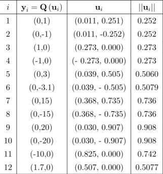
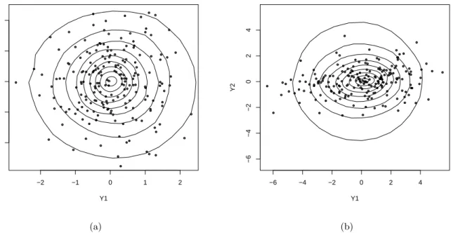
to get the corresponding quantile contour plot. Figure 1 (a) represent nine estimated contours (from 10% to 90%) ploted on the corresponding scatterplot.
● ● ● ● ● ● ● ● ● ● ● ● ● ● ● ● ● ● ● ● ● ● ● ● ● ● ● ● ● ● ● ●● ● ● ● ● ● ● ● ● ● ● ● ● ● ● ● ● ● ● ● ● ● ● ● ● ● ● ● ● ● ● ● ● ● ● ● ● ● ● ● ● ● ● ● ● ● ● ● ● ● ● ● ● ● ● ● ● ● ● ● ● ● ● ● ● ● ● ● ● ● ● ● ● ● ● ● ● ● ● ● ● ● ● ● ● ● ● ● ● ● ● ● ● ● ● ● ● ● ● ● ● ● ● ● ● ● ● ● ● ● ● ● ● ● ● ● ● ● ● ● ● ● ● ● ● ● ● ● ● ● ● ● ● ● ● ● ● ● ● ● ● ● ● ● ● ● ● ● ● ● ● ● ● ● ● ● ● ● ● ● ● ● ● ● ● ● ● ● −2 −1 0 1 2 −2 −1 0 1 2 Qn(u) Y1 Y2 ● ● ● ● ● ● ● ● ● ● ● ● ● ● ● ● ● ● ● ● ● ● ● ● ● ● ● ● ● ● ● ● ● ● ● ● ● ● ● ● ● ● ● ● ● ● ● ● ● ● ● ● ● ● ● ● ● ● ● ● ● ● ● ● ● ● ● ● ● ● ● ● ● ● ● ● ● ● ● ● ● ● ● ● ● ● ● ● ● ● ● ● ● ● ● ● ● ● ● ● ● ● ● ● ● ● ● ● ● ● ● ● ● ● ● ● ● ● ● ● ● ● ● ● ● ● ● ● ● ● ● ● ● ● ● ● ● ● ● ● ● ● ● ● ● ● ● ● ● ● ● ● ● ● ● ● ● ● ● ● ● ● ● ● ● ● ● ● ● ● ● ● ● ● ● ● ● ● ● ● ● ● ● ● ● ● ● ● ● ● ● ● ● ● ● ● ● ● ● ● −6 −4 −2 0 2 4 −6 −4 −2 0 2 4 Qn(u) Y1 Y2 (a) (b)
Figure 1: Quantile contour plots from 10% to 90% for observations given by (a) aN2(0, I2)
distri-bution, and (b) by aN2(0,Σ) distribution.
In order to make sure that contours adapt with the form of the scatter plot, we simulate 200
observations according to the multivariate normal distribution N2(0,Σ) with Σ =
5 0.4 0.4 1
!
.
Figure 1 (b) shows that the contours have a different form than those presented in Figure 1 (a), this confirms that they take well into account the various variances and covariances.
5.2 A second simulation: case of conditional spatial quantiles
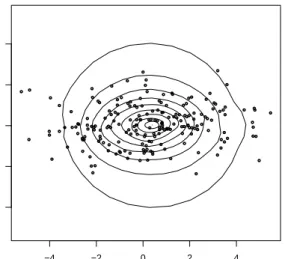
In order to see the behavior of the conditional spatial quantile estimators, while varying the vector
u, we have simulated 200 observations according to the following multivariate normal distribution:
Y1 Y2 X ∼N3 0,Γ = 5 0.2 0.4 0.2 1 0.9 0.4 0.9 1 .
In this example, we have fixed x= 0. Then for each value of u, we compute the estimator of the corresponding conditional spatial quantile.
● ● ● ● ● ● ● ● ● ● ● ● ● ● ● ● ● ● ● ● ● ● ● ● ● ● ● ● ● ● ● ● ● ● ● ● ● ● ● ● ● ● ● ● ● ● ● ● ● ● ● ● ● ● ● ● ● ● ● ● ● ● ● ● ● ● ● ● ● ● ● ● ● ● ● ● ● ● ● ● ● ● ● ● ● ● ● ● ● ● ● ● ● ● ● ● ● ● ● ● ● ● ● ● ● ● ● ● ● ● ● ● ● ● ● ● ● ● ● ● ● ● ● ● ● ● ● ● ● ● ● ● ● ● ● ● ● ● ● ● ● ● ● ● ● ● ● ● ● ● ● ● ● ● ● ● ● ● ● ● ● ● ● ● ● ● ● ● ● ● ● ● ● ● ● ● ● ● ● ● ● ● ● ● ● ● ● ● ● ● ● ● ● ● ● ● ● ● ● ● −4 −2 0 2 4 −4 −2 0 2 4 Qn(u|x=0) Y1 Y2
Figure 2: Conditional quantile contour plots from 10% to 90% for x= 0
Figure 2 shows that the conditional quantile contour plots from 10% to 90% ploted using the esti-mators of the conditional spatial quantiles adapt well with the form of the scatterplot. In addition, we know that the estimator of the spatial median (corresponding to u = (0,0)) converges asym-totically to the true median which is here for a multivariate normal distribution equal to the mean (0,0), so to check the quality of the estimator we have compared the estimated spatial median to the theoretical mean. Foru= (0,0), we haveQn(u |x= 0) = (0.08,−0.03), which is very close to (0,0).
Appendix
Proof of Theorem 4.1
• The first result can be deduced directly from the equation (11). If the observations are not lying in a single straight line inRd, then the conditional spatial quantile is the unique solution
yof the equation (11). Then we deduce that Qn(u|x) satisfy the following equation: n X i=1 Qn(u|x)−y ||Qn(u|x)−y||K x−Xi hn =u n X i=1 K x−Xi hn .
on Rd and it depends ony. One deduces that Qn(u|x) = arg min Q n X i=1 Φ(u,Yi−Q)K x−Xi hn
if and only if, for anyh∈Rd, we have
lim t→0+ " n X i=1 Φ(u,Yi−Qn(u|x) +th)K x−Xi hn − n X i=1 Φ(u,Yi−Qn(u|x))K x−Xi hn # ≥0.
However, for ally,h∈Rd such asy6= 0, we get:
lim t→0+ Φ(u,y+th)−Φ(u,y) t = limt→0+ ||y+th|| − ||y||+<u, th> t = < y ||y||+u,h> .
Moreover, for allh∈Rd and y= 0, we have
lim t→0+
Φ(u, th)−Φ(u,0)
t =|| h ||+<u,h> .
Thereafter, using those two properties on the previous inequality, we obtain:
X 1≤i≤n;Qn(u|x)6=Yi K x−Xi hn < Yi−Qn(u|x) ||Yi−Qn(u|x)|| +u,h> + X 1≤i≤n;Qn(u|x)=Yi K x−Xi hn (|| h ||+<u,h>)≥0.
Because this inequality is true for allh∈Rd, it is true also for−h. While replacinghpar−h
in the previous inequality, we obtain then:
X 1≤i≤n;Qn(u|x)=Yi K x−Xi hn (||h ||−<u,h>) ≥ X 1≤i≤n;Qn(u|x)6=Yi K x−Xi hn < Yi−Qn(u|x) ||Yi−Qn(u|x)|| +u,h> . (16)
On the other hand, using the Schwartz inequality, we get:
| ||h || ±<u,h>| ≤ || h ||+|<u,h>| ≤(1 +|| u ||)|| h ||.
Thus, inequality (16) is equivalent to
X 1≤i≤n;Qn(u|x)=Yi K x−Xi hn (1 +|| u||)||h || ≥ X 1≤i≤n;Qn(u|x)6=Yi K x−Xi hn < Yi−Qn(u|x) ||Yi−Qn(u|x)|| +u,h> . (17)
Because this inequality is true for allh∈Rd, we can choose in particular
h= Yi−Qn(u|x)
||Yi−Qn(u|x)||
+u. (18)
and if we put this value of h in equation (17), we get :
X 1≤i≤n;Qn(u|x)=Yi K x−Xi hn (1 +||u ||) ≥ X 1≤i≤n;Qn(u|x)6=Yi K x−Xi hn Yi−Qn(u|x) ||Yi−Qn(u|x)|| +u
Then we deduce the inequality (14).
Remark. The R-codes allowing to estimate spatial quantiles, conditional spatial quantiles and quantiles contour plots are available and can be asked to the authors.
References
Abdous, B. and Theodorescu, R. (1992). Note on the spatial quantile of a random vector.
Statistics and Probability Letter,13, 333-336.
Barnett, V. (1976). The ordering of multivariate data (with comments). Journal of Royal Statistical Society, Ser. A,139, 318-354.
Bedall, F.K. and Zimmermann, H. (1979). Algorithm AS 143, the Mediancenter. Applied Statistics,28, 325-328.
Brown, B. M., and Hettmansperger, T. P. (1987). Affine Invariant Rank Methods in the Bivariate Location Model. Journal of the Royal Statistical Society, Ser. B,49, 301-310.
Brown, B. M., and Hettmansperger, T. P. (1989). An Affine Invariant Bivariate Versions of the Sign Test. Journal of the Royal Statistical Society, Ser. B,51, 117-125.
Chakraborty, B. (2001). On affine equivariant multivariate quantiles. The Institute of Statistical Mathematics,53, 380-403.
Chaudhuri, P. (1992a). Multivariate location estimation using extension of R-estimates through
U-statistics type approach. Annals of Statistics,20, 897-916.
Chaudhuri, P. (1992b). Generalized regression quantiles: Forming a useful toolkit for robust linear regression. L1 Statistical Analysis and Related Methods, ed. Y. Dodge, Amesterdam:
Chaudhuri, P. (1996). On a geometric notation of quantiles for multivariate data. Journal of the American Statistical Association,91, 862-872.
De Gooijer, J. G., Gannoun, A. and Zerom, D. (2006). A multivariate quantile predictor. Com-munications in Statistics-Theory and Methods,35, 133-147.
Donoho, D. L. and Gasko, M. (1992). Breakdown properties of location estimates based on halfspace depth and projected outlyingness. Annals of Statistics,20, 1803-1827.
Eddy, W.F. (1985). Ordering of Multivariate Data. Computer Science and Statistics: The Interface, ed. L. Billard, Amesterdam: North-Holland, 25-30.
Efron, B. (1991). Regression percentiles using asymmetric squared error loss. Statistica Sinica,
1, 93-125.
Ferguson, T. (1967). Mathematical Statistics: A Decision Theoric Approach. Academic Press: New York.
Gannoun, A., Girard, S., Guinot, C. and Saracco, J. (2002). Reference curves based on non-parametric quantile regrassion. Statistics in Medecine,21, 3119-3135.
Gower, J. C. (1974). Algorithm AS 78: The Mediancenter. Applied Statistics,23, 466-470.
Koenker, R. and Basset, G. (1978). Regression Qantiles. Econometrica,46, 33-50.
Koenker, R. and Portnoy, S. (1987). L Estimation for linear models. Journal of the American statistical Association,82, 851-857.
Koltchinskii, V. (1997). M-estimation, convexity and quantiles. Annals of Statistics,25, 435-477.
Liu, R. Y., Parelius, J. M. and Singh, K. (1999). Multivariate analysis by data depth: Descriptive statistics, graphics and inference (with discussion). Annals of Statistics,27, 783-858.
Oja, H. (1983). Descriptive Statistics for Multivariate Trimming. Statistics and Probability Letters,1, 327-332.
Plackett, R. L. (1976). Comment on Ordering of multivariate data by V. Barnett. Journal of the Royal statistical Society, Ser.A,139, 344-346.
Reiss, R. D. (1989). Approximation distributions of order statistics with applications to nonpara-metric statistics. New York: Springer.
Serfling, R. (1980). Approximation theorem of mathematical statistics. New York: John Wiley.
Serfling, R. (2002). Quantile functions for multivariate analysis: approaches and applications.
Cahiers du GREThA
Working papers of GREThA
GREThA UMR CNRS 5113
Université Montesquieu Bordeaux IV
Avenue Léon Duguit
33608 PESSAC - FRANCE
Tel : +33 (0)5.56.84.25.75
Fax : +33 (0)5.56.84.86.47
www.gretha.fr
Cahiers du GREThA
(derniers numéros)2007-17 : BERTIN Alexandre, LEYLE David, Mesurer la pauvreté multidimensionnelle dans un pays en développement Démarche méthodologique et mesures appliquées au cas de l’Observatoire de Guinée Maritime
2007-18 : DOUAI Ali, Wealth, Well-being and Value(s): A Proposition of Structuring Concepts for a (real) Transdisciplinary Dialogue within Ecological Economics
2007-19 : AYADI Mohamed, RAHMOUNI Mohieddine, YILDIZOGLU Murat, Sectoral patterns of innovation in a developing country: The Tunisian case
2007-20 : BONIN Hubert, French investment banking at Belle Epoque: the legacy of the 19th
century Haute Banque
2007-21 : GONDARD-DELCROIX Claire, Une étude régionalisée des dynamiques de pauvreté Régularités et spécificités au sein du milieu rural malgache
2007-22 : BONIN Hubert, Jacques Laffitte banquier d’affaires sans créer de modèle de banque d’affaires (des années 1810 aux années 1840)
2008-01 : BERR Eric, Keynes and the Post Keynesians on Sustainable Development
2008-02 : NICET-CHENAF Dalila, Les accords de Barcelone permettent- ils une convergence de l’économie marocaine ?
2008-03 : CORIS Marie, The Coordination Issues of Relocations? How Proximity Still Matters in Location of Software Development Activities
2008-04 : BERR Eric, Quel développement pour le 21ème siècle ? Réflexions autour du concept de soutenabilité du développement
2008-05 : DUPUY Claude, LAVIGNE Stéphanie, Investment behaviors of the key actors in capitalism : when geography matters
2008-06 : MOYES Patrick, La mesure de la pauvreté en économie
2008-07 : POUYANNE Guillaume, Théorie économique de l’urbanisation discontinue
2008-08 : LACOUR Claude, PUISSANT Sylvette, Medium-Sized Cities and the Dynamics of Creative Services
2008-09 : BERTIN Alexandre, L’approche par les capabilités d’Amartya Sen, Une voie nouvelle pour le socialisme libéral
2008-10 : CHAOUCH Mohamed, GANNOUN Ali, SARACCO Jérôme, Conditional Spatial Quantile: Characterization and Nonparametric Estimation
La coordination scientifique des Cahiers du GREThA est assurée par Sylvie FERRARI et Vincent FRIGANT. La mise en page est assurée par Dominique REBOLLO.
Zuo, Y. and Serfling, R. (2000). General notions of statistical depth function. Annals of Statistics,