Outlier robust small area estimation under spatial
correlation
Timo Schmid
Nikos Tzavidis
Ralf Münnich
Ray Chambers
School of Business & Economics
Discussion Paper
Economics
Outlier robust small area estimation under spatial correlation
Timo Schmid*, Nikos Tzavidis**, Ralf M¨unnich***, and Ray Chambers****
*Institute of Statistics and Econometrics, Freie Universit¨at Berlin, Berlin, Germany
**Southampton Statistical Sciences Research Institute, University of Southampton, Southampton, UK ***Economic and Social Statistics Department, University of Trier, Trier, Germany
****National Institute for Applied Statistics Research Australia, University of Wollongong, Wollongong, Australia
Abstract
Modern systems of official statistics require the estimation and publication of business statistics for disaggregated domains, for example, industry domains and geographical regions. Outlier robust methods have proven to be useful for small area estimation. Recently proposed outlier robust model-based small area methods assume, however, uncorrelated random effects. Spatial dependencies, resulting from similar industry domains or geographic regions, often occur. In this paper we propose outlier robust small area methodology that allows for the presence of spatial correlation in the data. In particular, we present a robust predictive methodology that incorporates the potential spatial impact from other areas (domains) on the small area (domain) of interest. We further propose two parametric bootstrap methods for estimating the mean-squared error. Simulations indicate that the proposed methodology may lead to efficiency gains. The paper concludes with an illustrative application by using business data for estimating average labour costs in Italian provinces.
Keywords: Bias correction, projective and predictive estimators, spatial correlation, business surveys
1
Introduction
An important set of outputs for National Statistical Institutes (NSIs) are enterprise and trade statistics derived from business survey data. This has recently extended to small area/domain estimates for busi-ness statistics. During the last two decades there has been substantial growth in the development and application of model-based small area methods. However, small area estimation using business survey data presents a number of challenges. In this paper we focus on small area estimation when there are representative outliers (Chambers, 1986) in the sample data.
Outliers can invalidate the conventional parametric assumptions of Gaussian random effects and unit level errors of model-based methods, which in turn can impact the validity of model-based small area estimators. Sinha and Rao (2009) proposed a robust methodology for estimating the parameters of the nested error regression model that controls for the influence of outliers. An alternative approach that also uses influence functions to control the impact of outliers but is based on a different model was proposed
by Chambers and Tzavidis (2006). Both outlier robust estimators of Sinha and Rao (2009) and Chambers and Tzavidis (2006) are plug-in estimators. This implicitly assumes that all non-sample values follow a well-behaved working model, so that their sum can be predicted using an outlier robust fit of this working model to the outlier contaminated sample data. Chambers et al. (2014) refer to such methods as robust projective. Robust projective methods typically lead to biased estimators with lower variances. This is due to the fact that it is extremely unlikely that the non-sampled values in the target population are drawn from a distribution with the same mean as the sample non-outliers. To correct for this bias, Dongmo-Jiongo et al. (2013) and Chambers et al. (2014) proposed bias-corrected robust small area estimators with either local (area-specific) or global correction terms. Such bias-corrected estimators are referred to by Chambers et al. (2014) as robust predictive. The methodology used for building these robust predictive estimators goes back to the seminal work of Chambers (1986) and Welsh and Ronchetti (1998), in the sense that the local correction is obtained when the robust estimator is defined as the expected value of the small area mean under the outlier robust distribution function proposed by Welsh and Ronchetti (1998), while the global correction is motivated by extending the outlier robust population mean estimator of Chambers (1986) to a mixed effects working model.
In this paper we extend these ideas to outlier robust small area estimation under spatial correlation. Borrowing strength over space in small area estimation has been shown to offer some efficiency gains. One approach considers the use of geographically weighted regression (cf. Chandra et al., 2012 and Salvati et al., 2012), but this usually assumes that geo-referenced data at the individual level is available. This is hardly ever the case in business survey data. Another approach extends the nested error regression model by allowing for spatially correlated random effects that follow a simultaneously autoregressive (SAR) process (cf. Pratesi and Salvati, 2008). However, none of these methods considered estimation in the presence of outliers.
The approach we follow in this paper assumes a nested error regression model with correlated random effects that follow a SAR process. After reviewing the current literature on outlier robust small area estimation in Section 2, we present robust projective and robust predictive small area estimators under spatial correlation in Section 3. Mean Squared Error (MSE) estimation is studied in Section 4 by using two parametric bootstrap schemes that account for the spatial structure. The first scheme is based on a modified version of the parametric bootstrap proposed by Sinha and Rao (2009), whereas the second one is grounded on a modified version of the parametric bootstrap proposed by Dongmo-Jiongo et al. (2013). In Section 5 we empirically evaluate the proposed methodology by using a Monte-Carlo simulation under a range of scenarios. In Section 6 we apply the proposed methodology to business survey data from Italy. We conclude the paper by summarising our main findings and by providing some ideas for further research.
2
Outlier robust small area estimation
In this section we review the current literature on outlier robust small area estimation. We assume that the population of interestUof sizeN is divided intomnon-overlapping small areas of sizesNiand that
individual level data is available. The variable of interest is denoted byyj and is assumed to be linearly
related to a set of individual level auxiliary variablesxjand a set of area level covariateszj. The sample
sof sizenis selected from the population by using a sampling design which is non-informative given xj andzj. The population is divided intonsampled andN −nnon-sampled units, indexed bysand
r respectively. We use the subscriptito indicate the restriction to the specific areai, i. e.,si(ri)stands
for the set of sampled (non-sampled) units from areai. Furthermore, we assume that all small areas are sampled and that the small area population averages ofxiandzifori= 1, ..., mare known.
The industry standard approach to model-based small area estimation with unit level data uses the Battese, Harter and Fuller model (cf. Battese et al., 1988). This is a nested error regression model with area-specific random effects:
y = Xβ+Zv+e, (1)
v ∼ N(0,G),
ε ∼ N(0,R).
In (1)βis thek×1vector of regression parameters andvis the(m×1)vector of area specific random effects. The unit level errorseare assumed to be independently normally distributed with mean 0 and covariance R = σ2eIN. The covariance matricesGandRdepend on a vector of variance parameters
θ ={σv2, σ2e}. When the area effects are assumed to be independent, the covariance matrix of the random effects simplifies toG=σv2Im. Finally, since the two error termsv andeare independent, the
covari-ance matrix ofy is given byV =R+ZGZT. Letβˆ(θ)define the Best Linear Unbiased Estimator (BLUE) ofβandvˆ(θ)denotes the Best Linear Unbiased Predictor (BLUP) ofv(cf. Henderson, 1950 or Searle, 1971). In practice,θis unknown and needs to be estimated by using e.g. maximum likelihood or restricted maximum likelihood estimation. This leads to the empirical best versions ofβˆ(θˆ)andvˆ(θˆ). The EBLUP of the mean in small areaiis then given by
ˆ yEBLU Pi = Ni−1n X j∈si yj+ X j∈ri (xTjβˆ+ ˆvi) o . (2)
The EBLUP (2) is optimal when the model assumptions (1) hold. However, the presence of outliers in the data can invalidate these assumptions. The impact of outliers on estimation can be controlled by replacingβˆ andvˆby robust alternatives. One approach for achieving this was proposed by Sinha and Rao (2009). The paper suggested the use of the Huber influence functionψfor deriving robust versions of the maximum likelihood estimating equations leading to robust estimatorsβˆψ,θˆψ andvˆψ. An outlier robust version of (2) is ˆ yREBLU Pi =Ni−1n X j∈si yj+ X j∈ri (xTjβˆψ+ ˆviψ) o . (3)
Chambers et al. (2014) use the term robust projective to refer to estimators such as (3). Robust projective methods can be severely biased. The reason for the bias is not difficult to find. It is extremely
unlikely that the non-sampled values in the target population are drawn from a distribution with the same mean as the sample non-outliers, and yet these methods are built on precisely this assumption. Chambers (1986) recognised this dilemma and coined the concept of a representative outlier, i. e., a sample outlier that is potentially drawn from a group of population outliers, and hence, cannot be unit-weighted in estimation. He noted that representative outliers cannot be treated on the same basis in estimation as other sample data which are more consistent with the working model for the population, since such values can seriously destabilise the survey estimates. Chambers (1986) suggested an addition of an outlier robust bias correction term to a robust projective survey estimator, e. g., one based on outlier-robust estimates of the model parameters. Such bias-corrected estimators are referred to as robust predictive since they attempt to predict the contribution of the population outliers to the population parameter of interest.
Chambers et al. (2014) proposed a robust-predictive version of the REBLUP (3) based on the ideas of Chambers (1986) and Welsh and Ronchetti (1998). This estimator is
ˆ yCCSTi = ˆyREBLU Pi + (1− ni Ni )1 ni X j∈si ωiψφk n (yj−xTjβˆψ−ˆv ψ i )/ω ψ i o , (4)
where φk denotes a less restrictive influence function (|φ| ≥ |ψ|) with tuning constant k > 0 (cf.
Tzavidis et al., 2010) andωψi is the median absolute deviation of the residuals in areai. Note that setting
k = 0leads to the robust projective estimator (3). Hence, the bias-correction term depends only on local information from areai. Although estimator (4) has very good bias properties, it can suffer from high variability due to the fact that the correction term depends on the area-specific sample size which is usually fairly small. To amend this issue, Dongmo-Jiongo et al. (2013) proposed alternative robust predictive estimators that incorporate a global bias correction term which also depends on information from other small areas.
The first estimator of Dongmo-Jiongo et al. (2013) uses the ideas of Chambers (1986). The EBLUP (2) can be reformulated as a weighted linear function of the values in the samples(cf. Royall, 1976) by
ˆ yEBLU Pi = 1 Ni X j∈s wjEBLU Pyj = (wisEBLU P)Tys. (5)
Dongmo-Jiongo et al. (2013) used this result and derived the following robust predictive estimator
ˆ yCHAMi = ˆyREBLU Pi +Ni−1X j∈si ψk1 (wj−1)(yj −xTjβˆψ−vˆ ψ i ) (6) +Ni−1 m X h6=i h=1 X j∈sh ψk1 wj(yj−xTjβˆψ−ˆv ψ h) +N −1 i m X h=1 ψk2 $hvˆhψ where $h = P j∈siwj−Ni, h=i P j∈shwj, h6=i
andψkis the Huber influence function with tuning constantk. Dongmo-Jiongo et al. (2013) pointed out
that the robust predictor (6) converges to the EBLUP (2) for large values of the tuning constant and to the (3) for small values of the tuning constant. A second approach by Dongmo-Jiongo et al. (2013) uses the close relationship between the concept of conditional bias (CB) and the influence function (cf. Beaumont et al., 2013). The conditional bias, originally developed by Mu˜noz-Pichardo et al. (1995), measures the average influence of a unitjon an estimator. It is defined by
Bj yj, vh,β,θ
=E yˆi(θ)−yi|s, yj, vh
(7)
of a unitjin an areah(cf. Beaumont et al., 2013).
Using the concept of conditional bias, Dongmo-Jiongo et al. (2013) proposed a second robust pre-dictive estimator, ˆ yCBi = ˆyREBLU Pi +Ni−1X j∈si ψk1 (wj−1)(yj−xTjβˆψ−ˆv ψ i ) (8) +Ni−1 m X h6=i h=1 X j∈sh ψk1 wj(yj−xTjβˆψ−vˆ ψ h) +N −1 i m X h=1 $hˆvhψ.
3
Robust projective and predictive estimators with spatially correlated
random effects
The robust projective estimators (3) of Sinha and Rao (2009) and the robust predictive estimators (4), (6) or (8) of Chambers et al. (2014) and Dongmo-Jiongo et al. (2013) have all been developed under a nested error regression model that assumes uncorrelated random effects. Recent literature has demonstrated that in some cases borrowing strength over space can improve the efficiency of small area estimators. In this section we define robust projective and robust predictive estimators in the presence of correlated random effects.
One way to model spatial correlation is to allow for correlated random effects. We extend the nested error regression model along the lines of the work by Petrucci et al. (2005) and Pratesi and Salvati (2008) assuming a SAR process. The SAR model is defined by
y=Xβ+Zv+e, (9)
where the covariance matrices ofvandeare defined as in (1) but with
G = σ2v (I−ρWT)(I −ρW)−1
(10)
R = diag(σe2) (11)
respectively. The parameterρdescribes the strength of the spatial correlation andWis a given contiguity matrix that describes neighbourhood structure between the small areas. Under (9) an estimator of the
small area mean is defined by
ˆ
ySEBLU Pi =Ni−1X
j∈s
wspj yj =Ni−1(wissp)Tys. (12)
The weightswisspare given by
(wissp)T = 1Ts + (Ni−ni) xTriA+zTriB(Is−XsA) , (13) where A = XsTV−1X−1 XsTV−1 B = ZTR−1Z+G−1−1 ZTR−1
and1sis a vector of sizenwith
1s= 1, j ∈si 0, j ∈sh .
As we saw in Section 2, outliers can severely impact upon the estimation of model (9). In order to control their influence, a robust projective estimator of the small area mean under (9) uses robust ML equations for the estimation ofβ,θ,vandρleading to
ˆ ySREBLU Pi = Ni−1n X j∈si yj+ X j∈ri (xTjβˆψ,sp+ ˆvψ,spi ) o (14) = Ni−1 n niysi+ (Ni−ni)(xTriβˆψ,sp+zTrivˆ ψ,sp i ) o ,
where the superscript ψ points to the dependence of the estimator on the influence function and the superscriptsp indicates that the parameters depend on the spatial correlation parameterρ (cf. Schmid and M¨unnich, 2014). The robust projective estimator (14) is an extension of the Sinha and Rao estimator under (9), and hence, can suffer from the same bias problems. Thus, there is need to develop robust predictive estimators in the presence of spatial correlation.
The first robust predictive estimator we propose in this paper uses a local bias correction and is defined by ˆ ySCCSTi = ˆySREBLU Pi (15) +(1− ni Ni ) 1 ni X j∈si ωiψ,spφk n (yj−xTjβˆψ,sp−ˆv ψ,sp i )/ω ψ,sp i o ,
whereωψ,spi is the median absolute deviation of the residuals under the SAR model (9).
Two additional robust predictive estimators that use global bias correction terms are proposed under model (9). We start by noticing that (12) can be reformulated as follows (the detailed derivation is
available in the Appendix), ˆ ySEBLU Pi = ˆySREBLU Pi +N−1X j∈si wspj −1 yj−xTjβˆψ,sp−ˆv ψ,sp i (16) +N−1 m X h6=i h=1 X j∈sh wjsp yj−xTjβˆψ,sp−vˆ ψ,sp h +N−1 m X h=1 $sph vˆhψ,sp, where $sph = P j∈siw sp j −Ni, h=i P j∈shw sp j , h6=i .
The influence of outliers on (16) can be controlled by using a a Huber influence function in the last three terms of the estimator leading to the following robust predictive estimator,
ˆ ySCHAMi = ˆySREBLU Pi +Ni−1X j∈si ψk1 (wspj −1)(yj−xTjβˆψ,sp−ˆv ψ,sp i ) (17) +Ni−1 m X h6=i h=1 X j∈sh ψk1 wspj (yj−xTjβˆψ,sp−ˆv ψ,sp h ) +Ni−1 m X h=1 ψk2 $sph vˆhψ,sp .
The tuning constants used in the influence function are defined utilising the ideas in Dongmo-Jiongo et al. (2013). For small values of the tuning constantsk1andk2the robust predictive estimator converges
to the robust projective estimator (14), whereas for large tuning constants it converges to (12). A detailed discussion about the choice of the constants is given in Chambers et al. (2014) or Dongmo-Jiongo et al. (2013). Additional discussion is also provided in Section 5 of the present paper.
The second robust predictive estimator we propose in this paper is based on the concept of conditional bias, however it is developed under the SAR model. The conditional bias in this case is given by
Bj yj, vh,β,θ = 1 Ni(w sp j −1)(yj−xTjβ−vi) +Ni−1$ sp i vi, j∈si 1 Niw sp j (yj−xTjβ−vh) +N −1 i $ sp h vh, j∈sh with h6=i − 1 Niw sp j (yj −xTjβ−vi) +Ni−1$ sp i vi, j∈ri 1 Ni$ sp h vh, j∈rh with h6=i .
This leads to the following robust predictive estimator
ˆ ySCBi = ˆySREBLU Pi +Ni−1X j∈si ψk1 (wspj −1)(yj −xTjβˆψ,sp−vˆ ψ,sp i ) (18) +Ni−1 m X h6=i h=1 X j∈sh ψk1 wjsp(yj−xTjβˆψ,sp−vˆ ψ,sp h ) +N −1 i m X h=1 $hspˆvψ,sph .
4
Mean squared error estimation
Sinha and Rao (2009) and Dongmo-Jiongo et al. (2013) have already pointed out that the estimation of the mean squared error (MSE) is a challenging problem in the case of robust predictors. In this section we propose two parametric bootstrap schemes for estimating the MSE of the proposed robust predictive small area estimators we presented in Section 3. These bootstrap MSE estimators are extended to incorporate the spatial structure in the data. Both schemes are based on the work in Hall and Maiti (2006), Sinha and Rao (2009) and Dongmo-Jiongo et al. (2013). The difference between these bootstraps is in the mechanism used for generating the bootstrap population. In particular, the first bootstrap scheme generates bootstrap realisations of the random effectsv∗ and the error termse∗by using the non-robust estimates of the variance components (cf. Dongmo-Jiongo et al., 2013). In contrast, the second bootstrap uses robust estimates of the variance components for generating the bootstrap population (cf. Sinha and Rao, 2009). The comparison between these alternative bootstrap methods is considered for the first time in the present paper.
The steps of the bootstrap are as follows:
1. For givenβˆψ,sp,θˆandρˆestimated with the original sample generate area-specific random effects v∗ fromN(0, G( ˆθ,ρˆ))ande∗ fromN(0, R( ˆθ)). Use these to generate the bootstrap population and bootstrap sample,
y∗(b)=Xβˆψ,sp+Zv∗+e∗, (19)
and calculate the corresponding bootstrap population parameter for each areaiwhich we denote byτi(b).
For the first bootstrap method, we generate the bootstrap population by using non-robust estimatesθˆ= (ˆσv,σˆe) and ρˆ = ˆp. For the second parametric bootstrap approach we utilise robust estimates θˆ = (ˆσvψ,σˆeψ)andρˆ= ˆpψ. It is important to note that generation of the bootstrap population accounts for
spatial correlation between the random effects.
2. Using the bootstrap sample, estimate model (9). Using the estimated model parameters from the bootstrap sample, compute the corresponding small area estimator of the population mean in area
i,τˆi(b).τˆis a generic notation used to denote an estimator of the small area average.
3. UsingB bootstrap samples, the MSE estimator of the corresponding estimator in area i, τi, is
given by ˆ MSE(ˆτi) = 1 B B X b=1 ˆ τib−τib2.
5
Empirical evaluations
In this section, we present results from Monte-Carlo simulations that we carried out for assessing the performance of the proposed spatial robust estimators from Section 3. These estimators are compared
against those suggested by Chambers et al. (2014) and Dongmo-Jiongo et al. (2013) in Section 2. We further evaluate the performance of the MSE estimators.
Following Chambers et al. (2014), we generated population data form= 40small areas withNi = 100using a nested error regression model as follows
yj = 100 + 5xj+vi+eij. (20)
The covariates were generated from a log-normal-distribution withµx = 1andσx = 0.5. The unit level
errorseij and the random effectsvi were generated under a range of scenarios. In particular, following
Chambers et al. (2014), we focus on non-symmetric outlier contamination in the area and unit level errors. This is due to the fact that outlier robust projective estimators suffer from bias, especially under asymmetric contamination. The results in the case of symmetric contamination are available from the authors on request. Random effects and the individual errors were generated by using a mixture type contamination mechanism,
vi∼(1−γv)·N(0,G) +γv·N(9,20) (21)
eij ∼(1−γe)·N(0,6) +γe·N(10,150),
whereγv andγe control the percentage of outlier contamination in the population. Gis defined as in
(10) by
G=σ2v (I−ρWT)(I −ρW)−1
using σv2 = 3. We assume that the outlying areas are uncorrelated in (21). The spatial autoregressive parameterρis set to 0 for the non-spatial scenarios and to 0.8 for the scenarios with spatial correlation. W is defined by a8×5first-order contiguity matrix based on a rook structure (cf. Bivand et al., 2008). According to the rook structure, neighbours are cells to the horizontal and to the vertical of a cell, but not to the diagonal. W is row standardized to meet the requirements of the SAR model (cf. Petrucci et al., 2005). This leads to a row stochastic non-symmetric contiguity matrix. In the present of outliers in the data, the contamination levels are set toγv = 0.1andγe= 0.03. We investigated three spatial and three
non-spatial scenarios in total:
1. (0,0)- No contamination and no spatial correlation;γv =γe=ρ= 0.
2. (v,0)- Contamination only at the area level and no spatial correlation: vi ∼ N(0,3)for areas
1-36,vi ∼N(9,20)for areas 37-40,eij ∼N(0,6)andρ= 0.
3. (v, e) - Contamination at both levels and no spatial correlation: vi ∼ N(0,3)for areas 1-36,
vi ∼N(9,20)for areas 37-40,eij ∼0.97N(0,6) + 0.03N(10,150)andρ= 0.
4. (0,0)ρ- No contamination and spatial correlation;γv =γe = 0andρ= 0.8.
5. (v,0)ρ- Contamination only at area level and spatial correlation: vi ∼ N(0, G)for areas 1-36,
6. (v, e)ρ- Contamination and spatial correlation: vi ∼N(0, G)for areas 1-36, vi ∼N(9,20)for
areas 37-40,eij ∼0.97N(0,6) + 0.03N(10,150)andρ= 0.8.
Samples of sizeni = 5were selected from the population by simple random sampling without
replace-ment within each area. The population and sample sizes were held fixed for all areas. Each setting was repeated independently 500 times. The choice of small sample sizes is for two reasons. First, we investi-gate the proposed small area estimators under extreme cases. Second, the sample sizes in our application in Section 6 are approximately of similar size.
Several estimators of the small area population averages are evaluated. These are the standard EBLUP (2), which serves as a benchmark for other estimators, the spatial EBLUP (SEBLUP) (12), the robust EBLUP (REBLUP) (3) and the spatial robust EBLUP (SREBLUP) (14). Furthermore, the robust predictive estimators CCST (4), CHAM (6) and CB (8) are evaluated alongside their proposed spatial extensions SCCST (15), SCHAM (17) and SCB (18). Following Dongmo-Jiongo et al. (2013), the tuning constants for the bias-correction we used are equal to 3.
The following quality measures, over Monte-Carlo simulationsR, are used to evaluate the perfor-mance of an estimator of the average in areai,ˆτi,
• The relative bias (RB)
RB(ˆτi) = 1 R R X r=1 ˆ τi−τi τi .
• The relative root mean squared error (RRMSE) for each areai:
RRMSE(ˆτi) = v u u t 1 R R X r=1 ˆ τi−τi τi 2 .
Table 1 reports the RB and the RRMSE of the small area estimators. It can be observed that all esti-mators are unbiased in the scenarios without outliers(0,0)and(0,0)ρ. Furthermore, the results confirm
our expectations regarding the performance of the robust estimators. The robust projective estimators (REBLUP and SREBLUP) suffer from a negative bias in the case of non-symmetric outlier contamina-tion (cf. for instance scenarios[v, e]or[v, e]ρ). Chambers et al. (2014) have already pointed out that this is mainly caused by the implicit assumption of robust projective estimators which assume that the out-lier contamination component has zero expectation and that all outout-liers are observed in the sample. Our simulation scenarios have been specifically constructed to violate the assumptions of robust projective estimators. It is therefore natural that the robust projective estimators suffer from bias. On the other hand, the robust predictive estimators correct this bias. In particular, the robust (CCST and CHAM) and spatial robust predictive estimators (SCCST and SCHAM) have lower relative bias than the projective estimators (REBLUP and SREBLUP), especially in the areas 37-40. Furthermore, the CCST and SCCST estimators reveal slightly smaller relative bias compared to the CHAM and SCHAM estimators. In contrast, the CB and SCB estimators suffer from a relative large bias in the outlying areas 37-40 which is expected due to
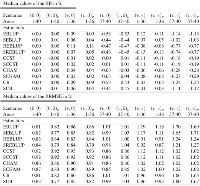
Table 1: Model-based simulation results: performance of predictors of small area means Median values of the RB in %
Scenarios (0,0) (0,0)ρ (v,0) (v,0)ρ (v,0) (v,0)ρ (v, e) (v, e)ρ (v, e) (v, e)ρ Areas 1-40 1-40 1-36 1-36 37-40 37-40 1-36 1-36 37-40 37-40 Estimators EBLUP 0.00 0.00 0.09 0.09 -0.53 -0.53 0.12 0.11 -1.14 -1.13 SEBLUP 0.00 0.01 0.06 0.04 -0.44 -0.44 0.07 0.05 -1.02 -1.03 REBLUP 0.00 0.00 0.11 0.11 -0.47 -0.47 -0.08 -0.08 -0.77 -0.77 SREBLUP 0.00 0.00 0.07 0.05 -0.43 -0.45 -0.13 -0.13 -0.74 -0.77 CCST 0.00 -0.00 0.01 0.02 0.00 0.01 -0.11 -0.11 -0.18 -0.19 SCCST 0.00 0.00 0.02 0.02 0.01 0.01 -0.11 -0.11 -0.19 -0.19 CHAM 0.00 0.00 0.04 0.04 -0.03 -0.03 -0.06 -0.06 -0.28 -0.28 SCHAM 0.00 0.00 0.03 0.02 -0.03 -0.04 -0.08 -0.08 -0.27 -0.29 CB 0.00 0.00 0.09 0.09 -0.53 -0.53 0.03 0.03 -1.24 -1.23 SCB 0.00 0.01 0.06 0.04 -0.44 -0.45 -0.01 -0.03 -1.11 -1.12
Median values of the RRMSE in %
Scenarios (0,0) (0,0)ρ (v,0) (v,0)ρ (v,0) (v,0)ρ (v, e) (v, e)ρ (v, e) (v, e)ρ Areas 1-40 1-40 1-36 1-36 37-40 37-40 1-36 1-36 37-40 37-40 Estimators EBLUP 0.81 0.82 0.86 0.86 1.01 1.01 1.19 1.18 1.70 1.69 SEBLUP 0.82 0.77 0.85 0.82 0.99 1.03 1.17 1.11 1.65 1.71 REBLUP 0.83 0.84 0.83 0.84 1.01 1.00 0.91 0.91 1.24 1.24 SREBLUP 0.84 0.79 0.84 0.79 0.98 1.04 0.92 0.87 1.21 1.27 CCST 0.92 0.92 0.93 0.93 0.86 0.86 1.12 1.12 1.02 1.02 SCCST 0.92 0.92 0.92 0.92 0.86 0.86 1.12 1.11 1.02 1.02 CHAM 0.86 0.86 0.90 0.91 0.86 0.86 1.02 1.02 1.02 1.02 SCHAM 0.87 0.83 0.90 0.89 0.85 0.85 1.02 1.00 1.02 1.02 CB 0.81 0.82 0.86 0.86 1.01 1.01 0.96 0.96 1.66 1.65 SCB 0.82 0.77 0.85 0.82 0.99 1.03 0.96 0.92 1.60 1.67
the contamination mechanism we use in the simulations. This bias is due to the non-robustified last terms in (8) and (18). Dongmo-Jiongo et al. (2013) present encouraging results for the CB estimator under a different data generation mechanism. Although the relative biases are small, we notice that SEBLUP and the SREBLUP estimators offer some bias reduction when compared respectively to the EBLUP and REBLUP estimators in the case of spatial scenarios.
We now turn to the RRMSE results in Table 1. As expected, in scenario(0,0)the robust predictive estimators CB and SCB are almost as efficient as the EBLUP, whereas the CHAM and SCHAM and the robust projective methods (REBLUP and SREBLUP) are somewhat less efficient.
In the case of the spatial scenario(0,0)ρthe spatial methods have a lower RRMSE compared to the corresponding non-spatial methods, for instance, the RRMSE of SCB is0.77%compared to0.82%for the CB estimator. For scenario (v, e)ρthe bias-corrected predictive spatial methods (SCCST, SCHAM and SCB) offer some gains in RRMSE when compared to the non-spatial predictive estimators (CCST, CHAM and CB) in the areas 1-36. It appears that accounting for the spatial structure in the estimation leads to some efficiency gains.
The CB and SCB estimators are slightly more efficient than the CCST or CHAM based methods in the areas 1-36 at the cost of a higher RRMSE in areas 37-40, where area and individual outliers occur at the same time. The bias part of the MSE is not negligible for the CB and SCB estimators in these areas. The CCST and CHAM spatial and non-spatial methods indicate a more consistent performance with low RRMSEs over all areas in scenarios (v, e) and (v, e)ρ. In contrast to the relative bias, the CHAM and SCHAM estimators perform slightly better in terms of RRMSE compared to the CCST and SCCST estimators. It seems that using information from other areas for the bias-correction in the CHAM methods helps to stabilise the results at the cost of a slightly higher bias compared to the CCST methods. These results illustrate the potentially beneficial effect of combining the spatial information with the bias correction offered by robust predictive estimators leading to more efficient results. However, robustness against outliers appears to be more important than incorporating the spatial structure in the estimation.
We now investigate the performance of the different MSE estimators. The objective of this part is twofold. First, we assess the performance of the proposed bootstrap methods for the spatial versions of the projective and predictive estimators. Second, we compare the performance of the robust and non-robust bootstrap methods in more detail in the case of spatial correlation. For both aims we focus on the scenarios with and without contamination invande.
MSE estimation is implemented with the parametric bootstrap methods presented in Section 4 with
B = 100bootstrap replicates. We denote by NonRobB and RobB the parametric bootstrap schemes where the v∗ ande∗ are generated by using non-robust or robust variance estimators respectively. We have also tested two selected scenarios,(0,0)ρand(v, e)ρ, by usingB = 500bootstrap replicates and the results did not change considerably . MSE results for some estimators such as for the EBLUP (using the Prasad-Rao estimator and the bootstrap MSE estimator), the CB (using the bootstrap MSE) and the SCB (using the bootstrap MSE) are excluded but are available from the authors on request.
Starting with the first aim, Table 2 presents the results for the MSE estimators and shows the me-dian values of their area-specific RB and RRMSE. We observe that both the robust and the non-robust spatial bootstrap methods work well for the scenarios without contamination. Under contamination, the bootstrap methods for the spatial estimators, SREBLUP, SCCST and SCHAM, lead to similar biases and stability compared to the bootstrap methods for the REBLUP, CCST and CHAM. Hence, the proposed MSE estimators that account for the additional spatial correlation in the data perform similarly to the bootstrap methods proposed by Sinha and Rao (2009) and Dongmo-Jiongo et al. (2013).
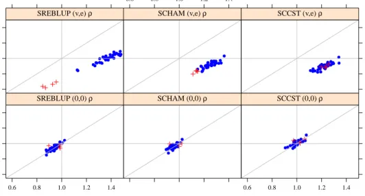
Having assessed the overall performance of the spatial versions of the bootstrap schemes, we now compare the proposed spatial robust and non-robust bootstrap methods explicitly. Figure 1 presents a more detailed picture of this comparison. It shows the ratio of the estimated non-robust MSE to the empirical (true) MSE (x-axis) against the ratio of the estimated robust MSE to the empirical (true) MSE (y-axis) for three estimators, the SREBLUP, the SCCST and the SCHAM. The crosses in the plot in-dicate the outlying areas 37-40. The vertical grey line inin-dicates the sector where the empirical MSE corresponds to the estimated non-robust MSE. Areas left to the vertical grey line suffer from underesti-mation, whereas areas right to the vertical line indicate overestimation. The same principle applies to the
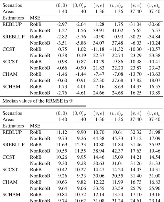
Table 2: Performance of MSE estimators in model-based simulations Median values of the RB in %
Scenarios (0,0) (0,0)ρ (v, e) (v, e)ρ (v, e) (v, e)ρ Areas 1-40 1-40 1-36 1-36 37-40 37-40 Estimators MSE REBLUP RobB -2.97 -2.64 1.28 1.75 -31.04 -30.66 NonRobB -1.27 -1.56 39.91 41.02 -5.65 -5.57 SREBLUP RobB -2.82 -5.76 -0.90 0.93 -30.25 -34.84 NonRobB -3.51 -5.86 34.07 37.48 -6.03 -10.24 CCST RobB 0.75 1.02 -11.18 -11.32 -10.30 -10.57 NonRobB 0.38 0.19 22.37 22.74 23.29 23.38 SCCST RobB 0.98 0.87 -10.29 -9.86 -10.38 -10.41 NonRobB -0.66 -0.90 21.83 22.20 23.87 23.43 CHAM RobB -1.46 -1.44 -7.47 -7.08 -13.70 -13.63 NonRobB -0.60 -0.91 27.30 27.68 17.82 18.07 SCHAM RobB -1.73 -4.01 -7.16 -8.69 -14.33 -16.55 NonRobB -2.76 -4.61 24.66 24.68 16.25 13.89 Median values of the RRMSE in %
Scenarios (0,0) (0,0)ρ (v, e) (v, e)ρ (v, e) (v, e)ρ Areas 1-40 1-40 1-36 1-36 37-40 37-40 Estimators MSE REBLUP RobB 11.12 9.90 10.70 10.61 32.32 31.98 NonRobB 9.73 9.26 44.38 45.33 17.12 17.09 SREBLUP RobB 11.69 12.33 10.80 11.84 31.46 35.92 NonRobB 10.55 11.55 38.94 42.37 17.63 19.46 CCST RobB 10.26 9.95 14.46 15.09 14.21 14.54 NonRobB 9.30 9.28 30.63 31.01 31.26 31.33 SCCST RobB 10.42 10.27 14.47 14.24 14.03 14.31 NonRobB 9.26 9.33 30.06 30.55 31.40 31.00 CHAM RobB 10.63 9.82 12.22 11.99 16.73 16.83 NonRobB 9.64 9.06 33.55 33.59 25.79 25.96 SCHAM RobB 10.84 10.72 12.14 13.54 17.10 19.16 NonRobB 9.74 10.62 31.08 31.24 24.61 23.14
horizontal grey line for the estimated robust MSE (underestimation below the grey line, overestimation above). The diagonal represents the sector where the estimated robust and non-robust MSE lead to the same results. Figure 1 reveals that the robust and the non-robust bootstrap schemes perform similarly in scenario (0,0)ρ. As a first comment in the scenario(v, e)ρ, we note that the non-robust bootstrap
method suffers from overestimation when estimating the MSE of the predictive estimators (SCHAM and SCCST). Second, the non-robust bootstrap method for the robust projective estimator (SREBLUP) overestimates the MSE for most areas, but not for the outlying areas 37-40 which is indicated by the crosses. In contrast, the robust version of the bootstrap MSE for the SREBLUP estimator is more stable, especially in the areas with only individual contamination (cf. areas 1-36), but underestimates the MSE for the outlying areas, because of a negative bias shown in Table 2. Third, the robust bootstrap MSE estimator performs consistently better than the non-robust version when used to estimate the MSE of the predictive estimators (SCCST and SCHAM). These results suggest that using the robust version of
Estimated Non Robust MSE / Empirical MSE
Estimated Rob
ust MSE / Empirical MSE
0.6 0.8 1.0 1.2 1.4 0.6 0.8 1.0 1.2 1.4 ● ● ● ● ● ● ● ● ● ● ●●●● ● ● ● ●●● ● ● ● ● ●●● ● ●●●● ● ● ● ● SREBLUP (0,0) ρ ● ● ● ● ● ●● ● ● ● ●●● ● ● ● ● ●● ● ● ●● ● ●●●● ●●●●●●● ● SCHAM (0,0) ρ 0.6 0.8 1.0 1.2 1.4 ●● ● ● ● ●● ● ● ● ● ●● ● ● ● ● ●● ●●● ●● ● ●● ● ●●●●●●●● SCCST (0,0) ρ ● ●● ●●● ●● ●●● ● ●●● ● ● ● ● ● ● ● ● ●● ● ● ● ● ● ● ● ●● ●● SREBLUP (v,e) ρ 0.6 0.8 1.0 1.2 1.4 ● ●●●●●● ● ●●●●●●●● ● ● ● ● ● ● ● ● ●● ● ● ● ● ● ● ● ● ● ● SCHAM (v,e) ρ 0.6 0.8 1.0 1.2 1.4 ● ● ● ● ● ● ●●●●●●● ●● ● ● ● ● ● ● ● ● ● ● ● ● ● ● ● ● ● ● ● ● ● SCCST (v,e) ρ
Figure 1: Robust and non-robust bootstrap estimators under spatial correlation.
the bootstrap for estimating the MSE of the predictive estimators appears to have appealing properties regarding the stability and bias in these scenarios.
6
Application: Small area estimation of average labour costs for small
and medium-sized enterprises in Italy
In Section 5 we evaluated the performance of different small area estimators under known contamination mechanisms. When using real data, however, the outlier contamination mechanism is unknown. In this section we employ the proposed methodology for estimating average labour costs for provinces in Italy. The focus here is on small and medium-sized enterprises with less than 100 employees as this group of firms is of great interest for economic policy (cf. Acs and Audretsch, 1988 or Sawyerr et al., 2003). In addition, for practical reasons, we only focus on one industry domain NACE 25 which refers to enterprises producing rubber and plastic products.
The business survey data of interest for this application come from Small and Medium Enterprises (SME) survey carried out annually by the Italian National Statistical Institute (ISTAT). In addition to the survey data, small area estimation is facilitated by the use of auxiliary information from the Italian Statistical Business Register (Asia - Archivio Statistico delle Imprese Attive). However, the use of business survey small area data is governed by strict confidentiality rules. To overcome this problem, in the application we use a synthetic dataset (TRItalia), which was created by using real data from the SME survey and the Asia register and preserves the structure of the original data (cf. Kolb et al., 2013). Similar to the Asia register, the TRItalia dataset consists of around 12,000 enterprises in the NACE 25 industry domain. Using the TRItalia dataset we selected a sample of 795 enterprises following a sampling design similar to the one of the SME survey. The design is a single stage stratified random sampling with strata defined by the cross-classification of administrative areas (NUTS 1) and a categorical variable for
Table 3: Summary statistics over provinces.
Min. 1st Qu. Median Mean 3rd Qu. Max.
Sample size 3.00 5.00 6.00 7.72 9.00 39.00
LCO (in KEUR) 0.01 9.67 50.68 216.10 176.60 15800.00
EMT 1.00 2.00 6.00 10.82 13.00 96.00
company size leading to 20 strata. In this application we are interested in providing reliable small area estimates of the average labour costs for enterprises in the NACE 25 sector for 103 Italian provinces. Similar to Fabrizi et al. (2013), the outcome of interest is the labour costs (LCO) in thousand Euro (KEUR).
Table 3 presents the distribution of the sample sizes, labour costs and number of employees (EMT) over provinces. The asymmetry in the unconditional distribution of labour costs is evident. It is more ap-propriate, though, to analyse the conditional distribution of labour costs given a set of auxiliary variables available.
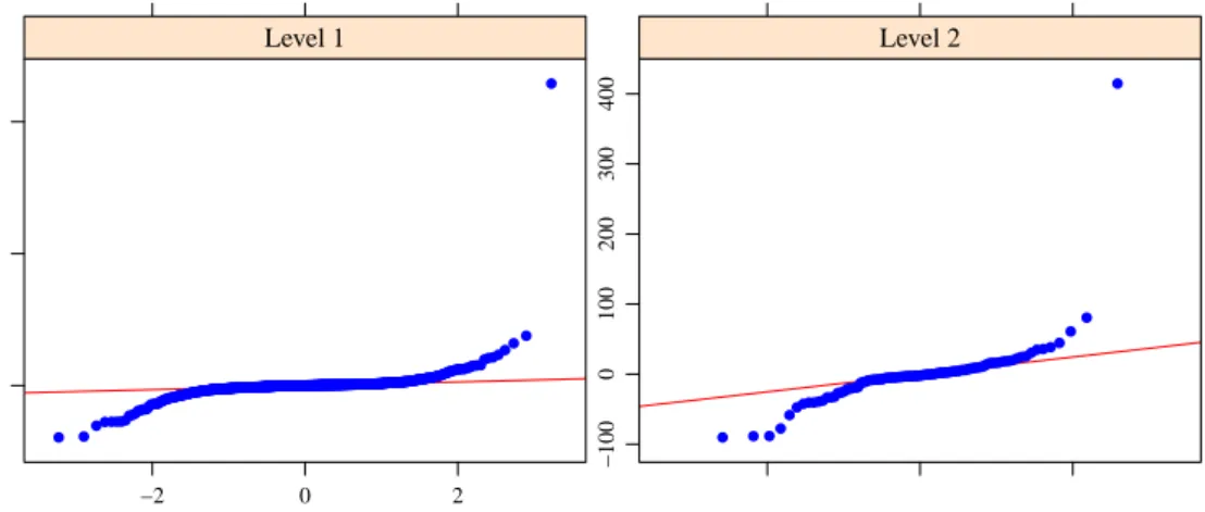
To do so, we use a 2-level random effects model (level 1 = enterprise; level 2 = province) for labour costs with random effects specified at the level of provinces. The auxiliary variables used in this model consist of the number of employees. To control for the stratified design of our sample, we further in-cluded the stratification variable defined by the cross classification between administrative areas and a categorical variable for company size. This defines 20 strata. This model provides a starting point which can later be extended. To assess departures from the model assumptions, Figure 2 presents normal prob-ability plots of level 1 and level 2 residuals. The figure indicates that the Gaussian assumptions of the
Theorical Quantiles Sample Quantiles 0 5000 10000 −2 0 2 ● ●●●●●● ●●●●●●●●●●●●●●●●●●●●●●●●●●●●●●●●●●●●●●●●●●●●●●●●●●●●●●●●●●●●●●●●●●●●●●●●●●●●●●●●●●●●●●●●●●●●●●●●●●●●●●●●●●●●●●●●●●●●●●●●●●●●●●●●●●●●●●●●●●●●●●●●●●●●●●●●●●●●●●●●●●●●●●●●●●●●●●●●●●●●●●●●●●●●●●●●●●●●●●●●●●●●●●●●●●●●●●●●●●●●●●●●●●●●●●●●●●●●●●●●●●●●●●●●●●●●●●●●●●●●●●●●●●●●●●●●●●●●●●●●●●●●●●●●●●●●●●●●●●●●●●●●●●●●●●●●●●●●●●●●●●●●●●●●●●●●●●●●●●●●●●●●●●●●●●●●●●●●●●●●●●●●●●●●●●●●●●●●●●●●●●●●●●●●●●●●●●●●●●●●●●●●●●●●●●●●●●●●●●●●●●●●●●●●●●●●●●●●●●●●●●●●●●●●●●●●●●●●●●●●●●●●●●●●●●●●●●●●●●●●●●●●●●●●●●●●●●●●●●●●●●●●●●●●●●●●●●●●●●●●●●●●●●●●●●●●●●●●●●●●●●●●●●●●●●●●●●●●●●●●●●●●●●●●●●●●●●●●●●●●●●●●●●●●●●●●●●●●●●●●●●●●●●●●●●●●●●●●●●●●●●●●●●●●●●●●●●●●●●●●●●●●●●●●●●●●●●●●●●●●●●●●●●●●●●●●●●●●●●●●●●●●●●●●●●●●●●●●●●●●●●●●●●●●●●●●●●●●●●●●●●●●●●●●●●●●●●●●●●●●●●●●●●●●●●●●●●●●●●●●●●●●●●●●●●●●●●●●●●●●●●●●●● ● ● Level 1 −2 0 2 −100 0 100 200 300 400 ● ● ●● ●●●●●●● ●●●●●●●●●●●●●●●●●●●●●●●●●●●●●●●●●●●●●●●●●●●●●●●●●●●●●●●●●●●●●●●●●●●●●●●●●●●●●●●●●●●●●●●●● ●● ● Level 2
Figure 2: Normal probability plots of level 1 (left) and level 2 (right) residuals.
model are violated. Furthermore, the Shapiro-Wilk test, which rejects the null hypothesis of normal distributed residuals (p-values: level 1 = 2.2e-16 and level 2 = 2.2e-16) confirms this. Using a robust estimation method to control for the influence of outliers may be advisable in this case.
Evidence of moderate spatial correlation in the data is also present. Following Pratesi and Salvati (2008), we compute two diagnostics for the presence of spatial autocorrelation. Moran’s I (cf. Moran,
Table 4: Values of the Moran’s I and Geary’s C tests. Value pvalue
Moran’s I 0.443 <1.9e−11
Geary’s C 0.509 <1.3e−11
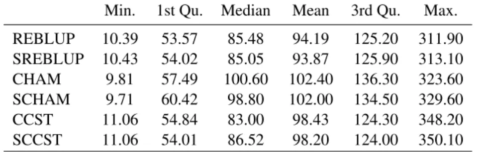
Table 5: Distribution of average labour costs (in KEUR) over provinces in Italy. Min. 1st Qu. Median Mean 3rd Qu. Max. REBLUP 10.39 53.57 85.48 94.19 125.20 311.90 SREBLUP 10.43 54.02 85.05 93.87 125.90 313.10 CHAM 9.81 57.49 100.60 102.40 136.30 323.60 SCHAM 9.71 60.42 98.80 102.00 134.50 329.60 CCST 11.06 54.84 83.00 98.43 124.30 348.20 SCCST 11.06 54.01 86.52 98.20 124.00 350.10
1950) is analogous to the correlation coefficient with values between -1 (strong negative spatial correla-tion) and 1 (strong positive spatial correlacorrela-tion), whereas 0 indicates no spatial correlation. Geary’s C (cf. Cliff and Ord, 1981) ranges between 0 (strong positive spatial correlation) and 2 (strong negative spatial correlation). Both tests, shown in Table 4, indicate the presence of positive spatial correlation in the data.
Estimates of average labour costs for each province are calculated by using the robust projective estimators REBLUP (3) and SREBLUP (14). We also computed estimates using the robust predictive estimators CCST (4) and CHAM (6), as well as their corresponding spatial extensions SCCST (15) and SCHAM (17). In order to save space, we omit the results for the standard EBLUP (2) and spatial EBLUP (12). We further exclude the CB (8) and SCB (18). These results are available from the authors on request.
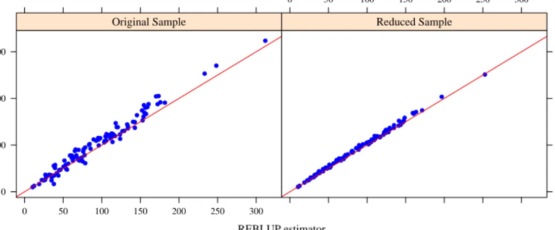
Table 5 presents the distribution of the estimated average labour costs in the sector of interest (NACE 25) for provinces in Italy. Our first observation is that there are some differences between the estimates obtained from the robust projective estimators (REBLUP and SREBLUP) and those from the robust predictive estimators (CCST, CHAM, SCCST and SCHAM). In order to further investigate the reason for these differences we performed the following sensitivity analysis. Using the Cook’s distance measure, we removed the most influential outliers from the sample. In total we removed 56 out of 795 observations. Using this reduced dataset, we recomputed the small area estimates. Figure 3 shows the robust projective estimator (REBLUP) (x-axis) against the robust predictive estimator (CHAM) (y-axis) for the reduced and original samples. The corresponding plot for the SREBLUP and SCHAM estimators is presented in Figure 4. We observe that the point estimates of the projective and predictive estimators are closer in the reduced sample. This behaviour can be explained by the fact that the restricted dataset includes a smaller number of outliers, and hence, the robust projective and predictive estimators provide closer results. In contrast, the stronger contamination in the original sample leads to systematically smaller estimates of the REBLUP and SREBLUP compared to the robust predictive estimators (CHAM and SCHAM). The
same picture holds also for the comparison between the projective estimators (REBLUP and SREBLUP) and the predictive estimators (CCST and SCCST). The results from this sensitivity analysis provide evidence that using a predictive estimator is possibly appropriate in this case.
REBLUP estimator CHAM estimator 0 100 200 300 0 50 100 150 200 250 300 ● ● ● ● ● ● ● ● ● ● ● ● ● ● ● ● ● ● ● ● ● ● ● ● ● ● ● ● ● ● ● ● ● ● ● ●● ● ● ● ● ● ● ● ● ● ● ● ● ●● ● ● ● ● ● ● ● ●●●●●●● ● ● ● ● ● ● ● ● ● ● ● ● ● ● ● ● ●● ● ●● ● ● ● ● ● ● ● ●● ● ● ● ● ● ● ● ● Original Sample 0 50 100 150 200 250 300 ● ● ● ● ● ● ● ● ● ● ● ● ● ● ● ● ● ● ● ● ● ● ● ● ● ● ● ● ● ●● ● ● ● ● ●● ● ● ● ● ● ● ● ● ● ● ● ● ● ● ● ● ● ● ● ● ● ●● ● ● ● ●● ● ● ● ● ● ●● ● ●●● ● ● ●● ● ● ● ● ● ● ●●● ● ● ● ● ●● ● ●● ● ● ● ● ● Reduced Sample
Figure 3: Differences between the projective estimator (REBLUP) and the predictive estimator (CHAM) for the reduced and original samples.
SREBLUP estimator SCHAM estimator 0 100 200 300 0 50 100 150 200 250 300 ● ● ● ● ● ● ● ● ● ● ● ● ● ● ● ● ● ● ● ● ● ● ● ● ● ● ● ● ● ● ● ● ● ● ● ●● ● ● ● ● ● ● ● ● ● ● ● ● ● ● ● ● ● ● ● ● ● ●●● ● ●●● ● ● ● ● ● ● ● ● ●● ● ● ● ● ● ● ● ● ● ● ● ●● ● ● ● ● ● ●● ● ● ● ● ● ● ● ● Original Sample 0 50 100 150 200 250 300 ● ● ● ● ● ● ● ● ● ● ● ● ● ● ● ● ● ● ● ● ● ● ● ● ● ● ● ● ● ●● ● ● ● ● ●● ● ● ● ● ● ● ● ● ● ● ● ● ● ● ● ● ● ● ● ● ● ●●● ● ● ●● ● ● ● ● ● ●● ● ●●● ● ● ●●● ● ● ● ●● ●●● ● ● ● ● ●● ● ●● ● ● ● ● ● Reduced Sample
Figure 4: Differences between the projective estimator (SREBLUP) and the predictive estimator (SCHAM) for the reduced and original samples.
MSE estimates, using the two bootstrap schemes we described in Section 4, are presented in Table 6. Based on the findings from the model-based simulations, in the presence of contamination we may expect overestimation of the MSE when bootstrapping from the non-robust estimates of the variance components. Indeed, the results suggest that this MSE estimator provides estimates that are very differ-ent to the ones obtained from the bootstrap method that uses the robust variance estimators. Examining further the MSE estimates, we note that the SREBLUP MSE estimates are lower than the corresponding REBLUP estimates. This suggests some efficiency gains obtained by incorporating the spatial informa-tion in estimainforma-tion. The same holds true when comparing the CHAM to the SCHAM and the CCST to the SCCST estimators. Considering the point and MSE estimates, we can conclude that the SCHAM or SCCST estimators appear to be a good choice for producing small area estimates of average labour
costs. The conservative analyst would choose the SCCST estimator, because of the slightly lower bias at the cost of a higher variance compared to the SCHAM estimator. In contrast, the SCHAM estimator offers more stability at the expense of a higher bias in relation to the SCCST estimator.
Table 6: MSE estimation MSE estimates using robust parametric bootstrap
Min. 1st Qu. Median Mean 3rd Qu. Max. REBLUP 19.12 44.10 51.38 54.74 63.80 105.40 SREBLUP 17.76 41.97 48.22 51.10 58.84 89.46 CHAM 20.38 49.84 56.33 59.75 69.27 113.10 SCHAM 18.36 45.29 54.09 55.65 64.90 97.99 CCST 25.95 117.10 168.90 185.70 243.20 447.90 SCCST 26.51 113.50 171.20 183.10 241.30 398.80 MSE estimates using non-robust parametric bootstrap
Min. 1st Qu. Median Mean 3rd Qu. Max.
REBLUP 5191 11890 14060 14240 15870 26980 SREBLUP 4843 9927 11110 11780 13650 26000 CHAM 5693 13210 15640 15680 17780 28300 SCHAM 4899 11310 12190 12760 14560 28970 CCST 6748 27670 38160 39780 50800 93640 SCCST 6278 25070 35510 37980 46460 83500
In Table 7 we investigate the estimates obtained from the SCHAM estimator in detail (SCCST esti-mates are available from the authors upon request). This table shows the mean labour costs per province divided by the average number of employees obtained from the synthetic register. An average employee in a small and medium-sized enterprise earns in Italy around 16,440 EUR per year. This is consistent with official results provided by ISTAT (cf. ISTAT, 2007). A more detailed picture of the spatial distri-bution of labour costs can be found in Figure 5. The figure shows the labour costs per employee for the 103 Italian provinces. As expected, we detect large regional disparities. The north-south divide in labour costs in Italy is clearly depicted in this figure.
7
Concluding remarks
The paper proposes extensions to the currently available outlier robust projective and robust predictive small area estimators in the presence of spatial correlation. The gains offered by the proposed method-ology are twofold. First, the outlier robust nature of the estimators reduces the impact of the misspecifi-cation of the model assumptions. Second, the methodology allows for modelling the spatial structure in the data. MSE estimation is performed by using two parametric bootstrap schemes that incorporate the
Table 7: Labour costs per employee per province (in KEUR) using the SCHAM estimator. Min. 1st Qu. Median Mean 3rd Qu. Max.
10 15 20 25 30 35 40
Figure 5: Mean labour costs per employee per province (in KEUR) using the SCHAM estimator.
spatial dimension. The results from the model-based simulations show that in the presence of contami-nation bootstrapping the data should be done as in Sinha and Rao (2009) by using the robust estimates of the variance components.
Currently, estimation relies on the a-priori choice of the tuning constants to be used in the influence functions. One could develop an adaptive (data driven) tuning constant to be used for small area predic-tion. This provides one avenue for future research. Moreover, the spatial small area estimators depend on the structure of a given contiguity matrixW. Another line for further work could be to investigate the effect of errors in specifying W on the estimation. Furthermore, the use of a bootstrap MSE esti-mator is computationally very demanding. Although the implementation of the proposed methodology is facilitated by the availability of a computationally efficient algorithm using C++ in R, its application in practice is challenging. Developing analytic MSE estimators similar to the one proposed in Chambers et al. (2014) offers an additional avenue for future research.
Acknowledgements
The research was conducted within the BLUE-ETS research project which is funded by the European Commission within the 7th Framework Programme. For more information on the project, we refer to the project pagehttp://www.blue-ets.eu. The authors are grateful to ISTAT and the BLUE-ETS project coordinator for kindly providing the business data. In addition, the research has received support from the InGRID (Inclusive Growth Research Infrastructure Diffusion) grant within the 7th Framework Programme. Furthermore, we would like to thank Dongmo-Jiongo et al. (2013) for providing R-code used in the simulations in this paper.
Appendix
In the appendix we show how the SEBLUP in equation (16) can be reformulated.
Niˆy SEBLU P i = X j∈s wjspyj = m X h=1 X j∈sh wjsp yj−xTjβˆψ,sp−vˆ ψ,sp h +x T jβˆψ,sp+ ˆv ψ,sp h = m X h6=i h=1 X j∈sh wjspˆvψ,sph + m X h6=i h=1 X j∈sh wspj yj−xTjβˆψ,sp−ˆv ψ,sp h + m X h6=i h=1 X j∈sh wjspxTjβˆψ,sp +X j∈si wspj yj−xTjβˆψ,sp−ˆv ψ,sp i +X j∈si wspj xTjβˆψ,sp+ ˆvψ,spi = m X h6=i h=1 X j∈sh wjspˆvψ,sph + m X h6=i h=1 X j∈sh wspj yj−xTjβˆψ,sp−ˆv ψ,sp h +X j∈s wjspxTjβˆψ,sp +X j∈si wspj yj−xTjβˆψ,sp−ˆv ψ,sp i +X j∈si wspj vˆiψ,sp = m X h6=i h=1 X j∈sh wjspˆvψ,sph + m X h6=i h=1 X j∈sh wspj yj−xTjβˆψ,sp−ˆv ψ,sp h +X j∈si wjspvˆψ,spi +X j∈Ui xTjβˆψ,sp+ ˆvψ,spi +X j∈si wjsp yj−xTjβˆψ,sp−vˆ ψ,sp i −Niˆvψ,spi = X j∈si yj+ X j∈ri xTjβˆψ,sp+ ˆviψ,sp +X j∈si wjsp yj−xTjβˆψ,sp−vˆ ψ,sp i −X j∈si yj−xTjβˆψ,sp−vˆ ψ,sp i + m X h6=i h=1 X j∈sh wspj yj−xTjβˆψ,sp−vˆ ψ,sp h +X j∈si wspj vˆiψ,sp−Nivˆiψ,sp+ m X h6=i h=1 X j∈sh wjspˆvψ,sph = X j∈si yj+ X j∈ri xTjβˆψ,sp+ ˆviψ,sp +X j∈si wspj −1 yj −xTjβˆψ,sp−vˆ ψ,sp i + m X h6=i h=1 X j∈sh wspj yj−xTjβˆψ,sp−ˆv ψ,sp h + X j∈si wjsp−Ni ˆ vψ,spi + m X h6=i h=1 X j∈sh wspj vˆhψ,sp = NˆySREBLU Pi +X j∈si wspj −1 yj −xTjβˆψ,sp−vˆ ψ,sp i + m X h6=i h=1 X j∈sh wspj yj−xTjβˆψ,sp−ˆv ψ,sp h + m X h=1 $sph vˆhψ,sp
References
Acs, Z. and D. Audretsch (1988). Innovation in large and small firms: An empirical analysis. American Economic Review 78 (4), 678–690.
county crop areas using survey and satellite data. Journal of the American Statistical Association 83 (401), 28–36.
Beaumont, J.-F., D. Haziza, and A. Ruiz-Gazen (2013). A unified approach to robust estimation in finite population sampling. Biometrika 100 (3), 555–569.
Bivand, R., E. Pebesma, and V. Gomez-Rubio (2008). Applied Spatial Data Analysis with R. New York: Springer.
Chambers, R. (1986). Outlier robust finite population estimation. Journal of the American Statistical Association 81, 1063–1069.
Chambers, R., H. Chandra, N. Salvati, and N. Tzavidis (2014). Outlier robust small area estimation.
Journal of the Royal Statistical Society: Series B 76 (1), 47–69.
Chambers, R. and N. Tzavidis (2006). M-quantile models for small area estimation. Biometrika 93 (2), 255–268.
Chandra, H., N. Salvati, R. Chambers, and N. Tzavidis (2012). Small area estimation under spatial nonstationarity. Computational Statistics and Data Analysis 56, 2875–2888.
Cliff, A. and J. Ord (1981). Spatial processes. London: Pion.
Dongmo-Jiongo, V., D. Haziza, and P. Duchesne (2013). Controlling the bias of robust small area estimators. Biometrika 100, 843–858.
Fabrizi, E., M. Ferrante, and C. Trivisano (2013). Small area estimation of labor productivity for the Italian manufacturing SME cross-classified by region, industry and size. Ersa conference papers, European Regional Science Association.
Hall, P. and T. Maiti (2006). On parametric bootstrap methods for small area prediction. Journal of the Royal Statistical Society: Series B 68 (2), 221–238.
Henderson, C. R. (1950). Estimation of genetic parameters. Annals of Mathematical Statistics 21 (2), 309–310.
ISTAT (2007). Conti economici delle imprese: Anno 2003. informazioni n. 8. Downloaded from http://www3.istat.it/dati/catalogo/20070827 01/inf 07 08 Conti economici delle imprese 2003.pdf (7th May 2014).
Kolb, J.-P., R. M¨unnich, F. Volk, and T. Zimmermann (2013). Best practice recommendations on vari-ance estimation and small area estimation in business surveys (final report), Chapter 5. TRItalia dataset, pp. 168–188. BLUE-ETS Project, FP7-SSH-2009-A, Deliverable 6.2.
Mu˜noz-Pichardo, J., J. Mu˜noz-Garcia, J. Moreno-Rebollo, and R. Pino-Mejias (1995). A new approach to influence analysis in linear models. Sankhya: The Indian Journal of Statistics, Series A (1961-2002) 57 (3), 393–409.
Petrucci, A., M. Pratesi, and N. Salvati (2005). Geographic information in small area estimation: Small area models and spatially correlated random area effects. Statistics in Transition 7 (3), 609–623. Pratesi, M. and N. Salvati (2008). Small area estimation: the eblup estimator based on spatially correlated
random area effects.Statistical Methods & Applications 17, 113–141.
Royall, R. (1976). The linear least-squares prediction approach to two-stage sampling. Journal of the American Statistical Association 71, 657–664.
Salvati, N., N. Tzavidis, M. Pratesi, and R. Chambers (2012). Small area estimation via m-quantile geographically weighted regression.Test 21 (1), 1–28.
Sawyerr, O., J. McGee, and M. Peterson (2003). Perceived uncertainty and firm performance in small and medium enterprises. International Small Business Journal 21 (3), 269–290.
Schmid, T. and R. M¨unnich (2014). Spatial robust small area estimation.Statistical Papers 55, 653–670. Searle, S. R. (1971). Linear Models. New York: Wiley.
Sinha, S. K. and J. N. K. Rao (2009). Robust small area estimation.The Canadian Journal of Statistics 37 (3), 381–399.
Tzavidis, N., S. Marchetti, and R. Chambers (2010). Robust estimation of small area means and quan-tiles. Australian and New Zealand Journal of Statistics 52 (2), 167–186.
Welsh, A. and E. Ronchetti (1998). Bias-calibrated estimation from sample surveys containing outliers.
Diskussionsbeiträge - Fachbereich Wirtschaftswissenschaft - Freie Universität Berlin
Discussion Paper - School of Business and Economics - Freie Universität Berlin
2015 erschienen:
2015/1 GÖRLITZ, Katja und Christina GRAVERT
The effects of increasing the standards of the high school curriculum on school dropout
Economics
2015/2 BÖNKE, Timm und Clive WERDT
Charitable giving and its persistent and transitory reactions to changes in tax incentives: evidence from the German Taxpayer Panel
Economics
2015/3 WERDT, Clive
What drives tax refund maximization from inter-temporal loss usage? Evidence from the German Taxpayer Panel
Economics
2015/4 FOSSEN, Frank M. und Johannes KÖNIG
Public health insurance and entry into self-employment Economics
2015/5 WERDT, Clive
The elasticity of taxable income for Germany and its sensitivity to the appropriate model
Economics
2015/6 NIKODINOSKA, Dragana und Carsten SCHRÖDER
On the Emissions-Inequality Trade-off in Energy Taxation: Evidence on the German Car Fuel Tax
Economics
2015/7 GROß, Marcus; Ulrich RENDTEL, Timo SCHMID, Sebastian SCHMON und Nikos
TZAVIDIS
Estimating the density of ethnic minorities and aged people in Berlin: Multivariate kernel density estimation applied to sensitive geo-referenced administrative data protected via measurement error