Western University Western University
Scholarship@Western
Scholarship@Western
Electronic Thesis and Dissertation Repository9-21-2018 10:00 AM
Tensor-based Hyperspectral Image Processing Methodology and
Tensor-based Hyperspectral Image Processing Methodology and
its Applications in Impervious Surface and Land Cover Mapping
its Applications in Impervious Surface and Land Cover Mapping
Boyu FengThe University of Western Ontario Supervisor
Wang, Jinfei
The University of Western Ontario Graduate Program in Geography
A thesis submitted in partial fulfillment of the requirements for the degree in Doctor of Philosophy
© Boyu Feng 2018
Follow this and additional works at: https://ir.lib.uwo.ca/etd
Part of the Geographic Information Sciences Commons, and the Remote Sensing Commons
Recommended Citation Recommended Citation
Feng, Boyu, "Tensor-based Hyperspectral Image Processing Methodology and its Applications in Impervious Surface and Land Cover Mapping" (2018). Electronic Thesis and Dissertation Repository. 5732.
https://ir.lib.uwo.ca/etd/5732
This Dissertation/Thesis is brought to you for free and open access by Scholarship@Western. It has been accepted for inclusion in Electronic Thesis and Dissertation Repository by an authorized administrator of
Abstract
The emergence of hyperspectral imaging provides a new perspective for Earth observation, in addition to previously available orthophoto and multispectral imagery. This thesis focused on both the new data and new methodology in the field of hyperspectral imaging. First, the application of the future hyperspectral satellite EnMAP in impervious surface area (ISA) mapping was studied. During the search for the appropriate ISA mapping procedure for the new data, the spectral unmixing based on nonnegative matrix factorization (NMF) achieved the best success. The simulated EnMAP image shows great potential in urban ISA mapping with over 85% accuracy.
Unfortunately, the NMF based on the linear algebra only considers the spectral information and neglects the spatial information in the original image. The recent wide interest of applying the multilinear algebra in computer vision sheds light on this problem and raised the idea of nonnegative tensor factorization (NTF). This thesis found that the NTF has more advantages over the NMF when work with medium- rather than the high-spatial-resolution hyperspectral image. Furthermore, this thesis proposed to equip the NTF-based spectral unmixing methods with the variations adopted from the NMF. By adopting the variations from the NMF, the urban ISA mapping results from the NTF were improved by ~2%.
Lastly, the problem known as the curse of dimensionality is an obstacle in hyperspectral image applications. The majority of current dimension reduction (DR) methods are restricted to using only the spectral information, when the spatial information is neglected. To overcome this defect, two spectral-spatial methods: patch-based and tensor-patch-based, were thoroughly studied and compared in this thesis. To date, the popularity of the two solutions remains in computer vision studies and their applications in hyperspectral DR are limited. The patch-based and tensor-patch-based variations greatly improved the quality of dimension-reduced hyperspectral images, which then improved the land cover mapping results from them. In addition, this thesis proposed to use an improved method
to produce an important intermediate result in the patch-based and tensor-patch-based DR process, which further improved the land cover mapping results.
Keywords
Nonnegative matrix factorization, nonnegative tensor factorization, hyperspectral image, spectral mixture analysis, dimension reduction, patch-based dimension reduction, tensor-patch-based dimension reduction.
Co-Authorship Statement
This thesis was prepared according to the integrated-article layout designed by the Faculty of Graduate Studies at Western University, London, Ontario, Canada. All the work stated in this thesis including methodology development, experimental testing, data analysis, modeling and writing draft manuscripts for publication was carried out by the author under the supervision of Dr. Jinfei Wang. Versions of Chapters 2, 3, and 4 have been accepted, submitted, or in preparation as co-authored peer reviewed journal papers. The coauthors can be found in the publication list below. Dr. Jinfei Wang provided the original conception of the application of the nonnegative matrix factorization method in remote sensing image processing. She proposed the urban feature extraction from high/medium resolution hyperspectral images for her NSERC Grant. Dr. Wang contributed in the development and formulation of methodology ideas and helped in establishing experimental procedures. She also provided valuable comments, editing and revision on the manuscripts, financial support, and software/hardware/data.
1. Feng, B. & Wang, J. (in preparation). Patch-based and tensor-patch-based dimension reduction methods for hyperspectral images.
2. Feng, B. & Wang, J. (under 1st round revision). Constrained nonnegative tensor factorization for spectral mixture analysis of hyperspectral imagery. IEEE Geoscience and Remote Sensing Letters.
3. Feng, B. & Wang, J. (in press). Evaluation of unmixing methods for impervious surface area extraction from simulated EnMAP imagery. IEEE Journal of Selected Topics in Applied Earth Observations and Remote Sensing.
Acknowledgments
Four years ago, I first came to Canada as a foreigner. Today I have made a lot of friends on the land far away from home and fulfilled my research responsibility in my Ph.D study. On this journey, I obtained a lot of help from different people, some of whom I may never have the chance to return the favor. Thus, I would like to express my gratitude to them here, because without their help I could not even think about finishing my thesis.
In the first place, I thank my parents who although not physically near me emotionally supported me to overcome the obstacles along the way. My advisor Dr. Jinfei Wang is the best mentor I can wish for, who assists me in both my study and my life in Canada. Her acute and open-minded research-thinking always inspires me. Her warm-hearted generosity gives me enormous courage along both of my research and life paths. Within her power, Dr. Jinfei Wang provides me great research opportunities and financial help, which I cannot thank her enough. I thank Dr. Ying Zhang from Canada Centre for Remote Sensing. Her trust in my research ability helps me to develop a comprehensive research project. Dr. Peter Ashmore from Geography Department and Dr. Imtiaz Shah from Engineering Department give me a lot of help in the design of my research. For their valuable advices and thoughtful ideas, I am very thankful. Also, I appreciate the suggestions provided by Dr. Livio Tornabene, from whom I learned to keep a down-to-earth research mind and never forget the most basic concepts.
I am thankful for the unrequired and timely help from my senior coworker, Dr. Chuiqing Zeng. His encouragement gives me great motivation in our research project. I am also obliged to my lab mates Chunhua Liao, Yang Song, Xiaodong Huang, Peter Crawford, Xiaoxuan Sun, and Matthew Roffey. They show me the most kindness and make the countlessly stressful office hours bright. We developed the most sincere friendship.
In the end, I have to thank the Geography Department in Western University for providing such a great opportunity for me to study here. The Geography Department provides me with great research resources, including powerful computing unit and
unparalleled dataset that I would not be able to use elsewhere. In addition, without the financial supports from the Geography Department, I will not be able to concentrate on my research as worrilessly as I was. I also thank the wonderful staffs in the Geography Department. First, I thank Ms. Lori Johnson, the graduate administrator. During the four years, she is always very helpful for questions I have regarding my study and life. I thank Mr. Joe Smrekar, who helps me countless times in problems concerning computer hardware and installation of software.
Table of Contents
Abstract ... i
Co-Authorship Statement... iii
Acknowledgments... iv
List of Tables ... xi
List of Figures ... xiii
List of Appendices ... xvii
List of Abbreviations ... xviii
1 Introduction ... 1
1.1 Research context ... 1
1.2 Research objectives ... 4
1.3 Studied images ... 5
1.4 Background ... 6
1.4.1 ISA/land cover mapping ... 6
1.4.2 Hyperspectral sensors ... 7
1.4.3 Problems with hyperspectral image ... 8
1.4.4 Multilinear algebra notation and preliminaries ... 12
1.5 Organization of the thesis ... 16
2 Evaluation of unmixing methods for simulated EnMAP hyperspectral imagery ... 23
2.1 Background ... 24
2.1.1 Previous studies on EnMAP ... 24
2.2 Objective ... 31
2.3 Methods... 31
2.3.1 Hyperspectral subspace identification ... 31
2.3.2 Endmember extraction and spectral mixture analysis ... 32
2.3.3 Abundance quantification ... 39
2.3.4 Evaluations ... 39
2.4 Experiments and Results ... 42
2.4.1 Study images ... 42
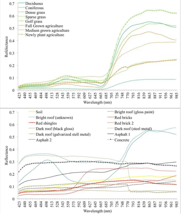
2.4.2 Reference spectra ... 44
2.4.3 Extracted endmember ... 48
2.4.4 ISA abundance and classification maps ... 50
2.5 Discussion ... 55
2.5.1 ISA abundance maps... 55
2.5.2 ISA classification maps... 60
2.5.3 Computation time... 63
2.6 Conclusion ... 65
3 Constrained nonnegative tensor factorization for spectral mixture analysis of hyperspectral image ... 75
3.1 Background ... 75
3.2 Objective ... 78
3.3 Methods... 79
3.3.2 Notations and tensor products ... 79
3.3.3 Matrix-vector nonnegative tensor factorization ... 80
3.3.4 Additional constraints ... 82
3.4 Experiments and results ... 84
3.4.1 Study areas, reference spectra, and research design ... 84
3.4.2 Extracted endmember ... 87
3.4.3 ISA abundances and classification maps ... 88
3.5 Discussion ... 92
3.5.1 ISA abundance maps... 93
3.5.2 ISA classification maps... 95
3.5.3 Comparison between the matrix-based and tensor-based methods ... 97
3.5.4 Computation time... 99
3.6 Conclusion ... 100
4 The application of spectral-spatial representation of hyperspectral image in dimension reduction ... 104
4.1 Background ... 104
4.1.1 Traditional dimension reduction methods ... 104
4.1.2 Spectral-spatial dimension reduction methods ... 107
4.2 Objective ... 110
4.3 Method ... 110
4.3.1 Dimension reduction methods ... 111
4.3.3 Computation complexity ... 122
4.3.4 Evaluation of the dimension reduction method ... 123
4.4 Experiments and results ... 124
4.4.1 Studied hyperspectral images and setup ... 124
4.4.2 Dimension reduction results ... 127
4.4.3 Classification results ... 130
4.5 Discussion ... 139
4.5.1 Comparison between patch-based and tensor-patch based dimension reduction methods ... 139
4.5.2 WRCM ... 140
4.5.3 Computation complexity ... 144
4.5.4 Other observations ... 145
4.6 Conclusion ... 145
5 General discussion and conclusions ... 151
5.1 Summary ... 151
5.2 Conclusions ... 153
5.3 Contributions... 154
Appendix A: Details of the CASI and simulated EnMAP spectral bands. ... 156
Appendix B: NMF update rules convergence proof ... 159
Appendix C: Theoretical justification of the LPP and NPE algorithms ... 163
Appendix D: Matlab code ... 166
List of Tables
Table 1-1: Studied image. ... 6
Table 2-1: Publications on the application of simulated EnMAP images. ... 25
Table 2-2: Reference spectra. ... 47
Table 2-3: Average minimum/median/difference spectral angle distance values (EnMAP). ... 50
Table 2-4: Average minimum/median/difference spectral angle distance values (Hydice). ... 50
Table 2-5: Reference and predicted ISA abundance linear regression parameters and classification overall accuracy (EnMAP). ... 52
Table 2-6: Reference and predicted ISA abundance linear regression parameters and classification overall accuracy (Hydice). ... 54
Table 2-7: Processing times in seconds. ... 64
Table 3-1: Average minimum/median/difference spectral angle distance values (EnMAP). ... 88
Table 3-2: Average minimum/median/difference spectral angle distance values (Hydice). ... 88
Table 3-3: Reference and predicted ISA abundance linear regression parameters and classification overall accuracy (EnMAP). ... 90
Table 3-4: Reference and predicted ISA abundance linear regression parameters and classification overall accuracy (Hydice). ... 92
Table 3-6: Comparison between NMF-based and MVNTF-based methods (Hydice). .... 98
Table 3-7: Processing times in seconds. ... 100
Table 4-1: Highest overall accuracy among patch-based dimension reduction methods. ... 134
Table 4-2 Highest overall accuracy among tensor-patch-based DR methods. ... 137
Table 4-3: Producer’s accuracies for patch-based DR methods (CASI image)... 141
Table 4-4: User’s accuracies for patch-based DR methods (CASI image). ... 141
Table 4-5: Producer’s accuracies for tensor-patch-based DR methods (CASI image). . 142
Table 4-6: User’s accuracies for tensor-patch-based DR methods (CASI image). ... 142
Table 4-7: Producer’s accuracies for patch-based DR methods (AVIRIS image). ... 142
Table 4-8: User’s accuracies for patch-based DR methods (AVIRIS image). ... 143
Table 4-9: Producer’s accuracies for tensor-patch-based DR methods (AVIRIS image). ... 143
Table 4-10: User’s accuracies for tensor-patch-based DR methods (AVIRIS image). .. 144
List of Figures
Figure 1-1: Panchromatic/orthophoto/multispectral VS. hyperspectral images. ... 2
Figure 1-2: Hyperspectral image matricization (3D cube to 2D matrix). ... 4
Figure 1-3: Spectral mixture analysis illustration of one pixel. ... 9
Figure 1-4: Principal component analysis illustration. ... 11
Figure 1-5: Swiss roll dataset illustration: ... 12
Figure 1-6: Fibers and slices of a third-order tensor: ... 13
Figure 1-7: Tensor decomposition illustration:... 16
Figure 1-8: Relationship among the three sub-studies. ... 17
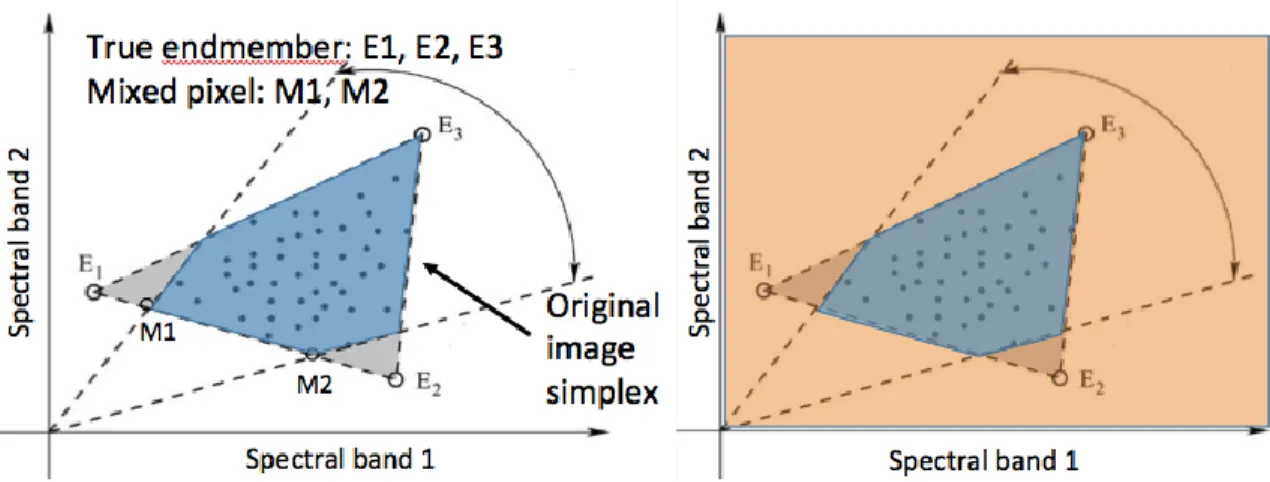
Figure 2-1: Original image simplex and solution space. ... 28
Figure 2-2: Sparse abundance matrix. ... 29
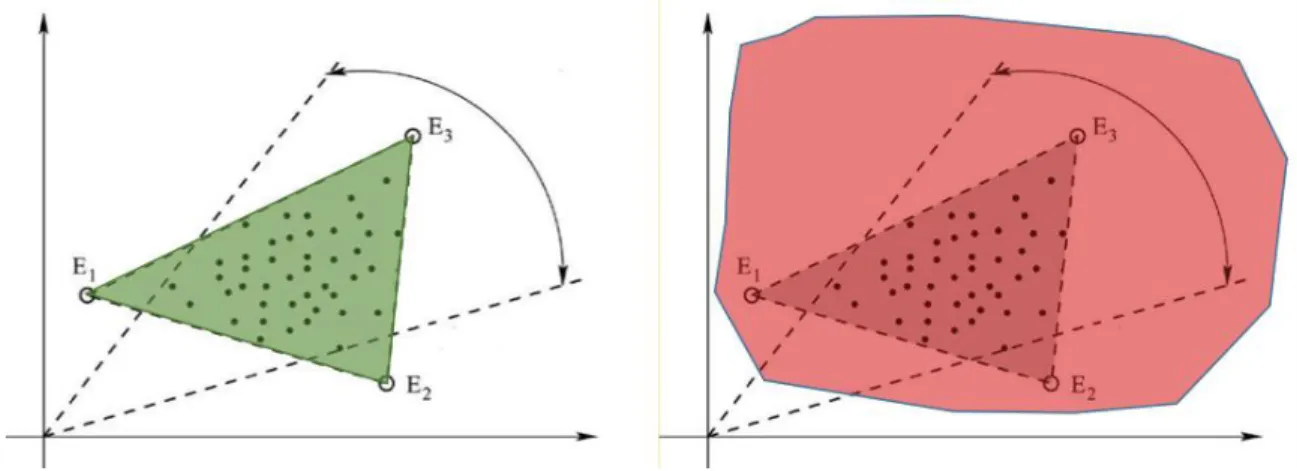
Figure 2-3: Left: preferred solution; Right: not preferred solution simplex. ... 30
Figure 2-4: Nonlinear effect (Yokoya, Chanussot and Iwasaki 2014). ... 30
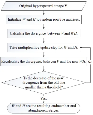
Figure 2-5: Nonnegative matrix factorization algorithm flowchart. ... 36
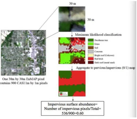
Figure 2-6: Generate reference map from the CASI image. ... 41
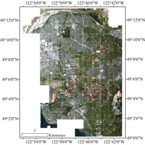
Figure 2-7: The simulated EnMAP image with RGB combination (Surrey, BC, Canada). ... 43
Figure 2-8: Hydice urban image with RGB combination (Copperas Cove, TX, USA). .. 44
Figure 2-10: Reference endmembers for Hydice urban image. ... 47
Figure 2-11: The best impervious surface area abundance maps from each spectral mixture analysis method (EnMAP). ... 58
Figure 2-12: The best impervious surface area abundance maps from each spectral mixture analysis method (Hydice). ... 59
Figure 2-13: The best impervious surface area classification maps from each spectral mixture analysis method (EnMAP). ... 62
Figure 2-14: The best impervious surface area abundance maps from each spectral mixture analysis method (Hydice). ... 63
Figure 3-1: BTD (Qian et al. 2017). ... 77
Figure 3-2: MVNTF (Qian et al. 2017). ... 77
Figure 3-3: Matrix vector nonnegative tensor factorization algorithm flowchart. ... 82
Figure 3-4: The cropped simulated EnMAP image in RGB. ... 85
Figure 3-5: The best impervious surface area abundance maps from each spectral mixture analysis method (EnMAP). ... 94
Figure 3-6: The best impervious surface area abundance maps from each spectral mixture analysis method (Hydice). ... 95
Figure 3-7: The best impervious surface area classification maps from each spectral mixture analysis method (EnMAP). ... 96
Figure 3-8: The best impervious surface area abundance maps from each spectral mixture analysis method (Hydice). ... 97
Figure 4-2: Flowchart of the TLPP and TNPE methods... 116
Figure 4-3: Spatial neighbors of three cases ... 117
Figure 4-4: Flowchart to calculate the IPD with a 3 × 3 spatial window (Pu et al. 2014). ... 118
Figure 4-5: Example results from RCM. ... 120
Figure 4-6: Example results from WRCM... 122
Figure 4-7: Surrey, BC, CASI hyperspectral image in RGB. ... 125
Figure 4-8: Indian Pines, AVIRIS hyperspectral image in RGB. ... 125
Figure 4-9: First band of the dimension-reduced images with the window size (in parentheses) that has the best overall accuracy (CASI image). ... 128
Figure 4-10: First band of the dimension-reduced images with the window size (in parenthesis) that has the best overall accuracy (AVIRIS image). ... 128
Figure 4-11: First band of the dimension-reduced images with the window size (in parentheses) that has the best overall accuracy (CASI image). ... 129
Figure 4-12: First band of the dimension-reduced images with the window size (in parentheses) that has the best overall accuracy (AVIRIS image). ... 130
Figure 4-13: Training and testing samples (CASI image). ... 131
Figure 4-14: Training and testing samples (AVIRIS image). ... 131
Figure 4-15: Original image and PCA (preserved dimensions) image classification (CASI image). ... 132
Figure 4-16: Ground truth, original image classification, and PCA (preserved dimensions) image classification (AVIRIS image). ... 133
Figure 4-17: Land cover classification maps derived from patch-based
dimension-reduced images (CASI image). ... 135
Figure 4-18: Classification maps for patch-based DR results (AVIRIS image) ... 136
Figure 4-19: Classification maps for tensor-patch-based DR results (CASI image). ... 138
List of Appendices
Appendix A: Details of the CASI and simulated EnMAP spectral bands. ... 156
Appendix B: NMF update rules convergence proof ... 159
Appendix C: Theoretical justification of the LPP and NPE algorithms ... 163
Appendix D: Matlab code ... 166
List of Abbreviations
SMA:spectral mixture analysis.
DR: dimension reduction. ISA: impervious surface area.
V-I-S: vegetation-impervious surface-soil.
PPI: pixel purity index.
ICA: independent component analysis. NMF: nonnegative matrix factorization.
sNMF: nonnegative matrix factorization with the sparseness constraint.
vNMF: nonnegative matrix factorization with minimum the volume constraint. rNMF: nonnegative matrix factorization with the robust nonlinear constraint.
HFC: Harsanyi–Farrand–Chang method. SAD: spectral angle distance.
NTF: nonnegative tensor factorization.
CP decomposition: CANDECOMP/PARAFAC decomposition. BTD: block term decomposition.
MVNTF: matrix-vector nonnegative tensor factorization.
sMVNTF: matrix-vector nonnegative tensor factorization with the sparseness constraint. vMVNTF: matrix-vector nonnegative tensor factorization ith the minimum volume constraint.
rMVNTF: matrix-vector nonnegative tensor factorization with the robust nonlinear constraint.
PCA: principle component analysis.
MDS: multidimensional scaling.
kNN: k nearest neighbors. LLE: locally linear embedding.
NPE: neighborhood preserving embedding. LE: Laplacian eigenmaps.
LPP: locality preserving projections.
TLPP: tensor locality preserving projections.
TNPE: tensor neighborhood preserving embedding. IPD: image patch distance.
RCM: region covariance matrix.
1
Introduction
1.1
Research context
The urban impervious surface area (ISA) 1 and land cover are significant environment indicators (Arnold Jr and Gibbons 1996). Strong relations between the ISA/land cover and the urban hydrologic cycle (Miller et al. 2014, Arnold Jr and Gibbons 1996, Li et al. 2009, Loperfido et al. 2014, Pauleit, Ennos and Golding 2005, Leopold 1968), urban microclimate (Yuan and Bauer 2007, Voogt and Oke 2003, Zhou et al. 2014, Carlson and Arthur 2000, Xian and Crane 2006), and urban biodiversity (Seto, Güneralp and Hutyra 2012, McKinney 2008) have been found. The increase in urban ISA decreases the surface infiltration rate, increases water runoff, and triggers high peak streamflow (Paul and Meyer 2001). The land cover governs the behavior of the water runoff from urbanized and industrial areas discharges conveying large amount of nutrients, metals, pesticides, and other contaminants to streams (Karn and Harada 2001, Leopold 1968). Some impacts of the ISA on the urban energy budget are that, compared to previous areas, ISA absorbs more short-wave radiation, impedes release of long-wave energy to atmosphere, and increase the long-wave radiation to surrounding environment (Zhou et al. 2014), causing the urban heat island (Xu 2010). The land cover leads to intra-urban microclimate differences (Buyantuyev and Wu 2010). The increase of ISA also contributes to the loss of habitat, biomass, and carbon storage, jeopardizing biodiversity and ecosystem productivity (Seto et al. 2012). In addition, it has been found that the lack of urban green space due to ISA increase is disadvantageous to human physical activity, psychological well-being and the general public health of urban residents (Wolch, Byrne and Newell 2014). Furthermore, in the age of rapid urbanization, the urban ISA and land cover experience intense changes over the short time. Thus, in order to achieve urban sustainability, it is important to obtain up-to-date knowledge about the composition and distribution of urban ISA and land cover distribution.
1Impervious surfaces are mainly artificial structures that are covered by impenetrable materials such as asphalt and concrete.
Prior to the appearance of remote sensing, ISA/land cover studies were relatively disordered. For a long time, the ISA/land cover data were collected by agencies at various governmental levels under different standards, with little-to-no communication existing among them. This fact resulted in a confusing situation that forbid duplicated or shared work even in situations where the data were collected under similar premises (Anderson 1976). Additionally, at that time, the ISA/land cover data were obtained through ground surveys, which was labor intensive and time-consuming. Since the development of remote sensors, the remote sensing data has gradually become the mostly chosen source of information of information for ISA/land cover study.
The spectrum of a material is a plot of the percentage of reflectance, or emissivity, across a range of wavelengths. As all materials reflect, emit, transmit and absorb electromagnetic radiation based on the inherent physical structure and chemical composition of the material and the wavelength of the radiation (Vagni 2007), the spectrum of each material is unique. Remote sensors are designed to identify such spectral signatures and perform land cover mapping. The design of hyperspectral imaging of hundreds of spectral bands outperforms the traditional panchromatic (1 band), orthochromatic (usually has 3 bands), and multispectral (usually has 4~10 bands) sensors by providing more detailed spectral signatures (Figure 1-1).
In high demand, new hyperspectral sensors have been constantly designed. The near-future hyperspectral satellite project is Germany’s environmental mapping and analysis program (EnMAP). Studies are needed for the future hypersepctral satellite, in order to take advantage of its new features. Depending on the new features and the practical objectives, different image processing procedures can be tested to find the appropriate solutions for the new hypersepctral satellite in different situations. This thesis focused on the ISA mapping ability of the future EnMAP image.
As the information in high dimensional data (e.g. hyperspectral images) are often redundant and contaminated by noise (Zhuo, Cheng and Zhang 2014), the efficient ISA/land cover mapping requires powerful processing methods. The majority of the current hyperspectral processing methods are applied in absence of the use of spatial information. Based on linear algebra, the spatial coordinates of pixels are often reconstructed into vectorized index during the process, which converts the original hyperspectral 3D cube into a 2D matrix (Figure 1-2). From now on, the methods based on linear algebra are referred to as the matrix-based methods. Fortunately, from the late 2000s, multilinear algebra is widely being studied in computer vision. Although the application of multilinear algebra in remote sensing is still limited, this trend sheds light on the possibility of improving series of hyperspectral image processing methods by preserving the spatial information. From now on, the methods based on multilinear algebra are referred to as the tensor2-based methods. In addition, inspired by the different variations of the widely used matrix-based hyperspectral image processing methods, I proposed to adopt them in tensor-based methods, which may also improve the final results. This thesis focused on improving two typical hyperspectral problems: spectral unmixing and dimension reduction, by tensor-based methods.
Figure 1-2: Hyperspectral image matricization (3D cube to 2D matrix).
1.2
Research objectives
The main objective of this thesis is to evaluate current, and develop new, remote sensing methodologies, on current/future hyperspectral images, in order to produce ISA/land cover maps with high accuracy and fidelity. Specifically, three sub-objectives for the three sub-studies are:
(1) To find the appropriate image processing methods for ISA mapping using the new simulated hyperspectral satellite EnMAP image.
(2)To upgrade one of the most robust spectral unmixing methods (nonnegative matrix factorization) from a matrix-based version to a tensor-based one and further improve the tensor-based method by incorporating additional constraints that have been previously added to the matrix-based method, to test improvement in the ISA mapping results.
(3) To upgrade the graph-based dimension reduction method to its tensor version and further improve the tensor-based method by the use of a new method for the intermediate results of adjacency graph/weight matrix, in the hope to improve the land cover mapping results.
Corresponding to the objectives, the following research questions are the focus of this thesis:
(1)Aiming to obtain accurate ISA maps, what processing procedures are appropriate for the new satellite EnMAP data when no additional data are available?
(2)How does the newly developed tensor-based spectral unmixing method assist the ISA mapping compared to the matrix-based method?
(3)Can the variations of the matrix-based spectral unmixing methods be implemented to the tensor-based methods? After this implementation, will the results of the tensor-based methods be improved?
(4)How does the newly developed spectral-spatial dimension reduction methods assist the land cover mapping compared to the matrix-based method?
(5)By improving the intermediate results (adjacency graph/weight matrix) of the tensor-based dimension reduction methods, can the final land cover mapping be improved?
1.3
Studied images
The quality of the final ISA and land cover maps relates to not only the discussed method, but also the studied hyperspectral images. Different processing methods may be appropriate solutions for different hyperspectral images. Features like spatial and spectral resolutions and locations (e.g. urban or suburban) of the hyperspectral images impact the outcomes for certain methods. Thus, one can seldom only work on image processing methods without considering the target. In order to comprehensively analyze the performances of studied methods regarding to different images, the hyperspectral images used for the analysis are carefully selected (Table 1-1). Firstly, this thesis provides spectral unmixing on one simulated EnMAP image (2013), whose results are valuable for the future application of the new hyperspectral sensor. The Copperas Cove, TX, Hydice image (1995) was also used in the spectral unmixing, for comparison purpose. As the EnMAP and Hydice images have different spatial and spectral resolution, they were able to reflect the different preferences of the spectral unmixing methods. In the dimension reduction experiments, the widely used Indian Pines AVIRIS image (1992) was used along with one newer CASI image (2013). The spectral band information of the EnMAP
and CASI data is provided in Appendix A. The spectral band information of the Hydice and AVIRIS data are open online (http://lesun.weebly.com/hyperspectral-data-set.html ).
Table 1-1: Studied image.
Methods Platforms Location type Spatial resolution Spectral resolution Temporal resolution Simulated EnMAP Spectral unmixing Satellite Urban-suburban 30m 88 bands (420-990nm) 4 days Hydice Spectral unmixing
Airplane Urban 2m 162 bands (400-2500nm)
NA AVIRIS Dimension
reduction
Airplane Agriculture 20m 200 bands (400-2500nm)
NA CASI Dimension
reduction
Airplane Urban 1m 72 bands (360-1050nm)
NA
1.4
Background
1.4.1
ISA/land cover mapping
An ISA/land cover mapping literature search on Google Scholar, with approximately 80% - 90% of the articles being published in English, displayed literature from the 1990s to 2018. The majority of current ISA/land cover mapping used multispectral images, instead of hyperspectral images. This was largely due to a lack of hyperspectral sensors suitable for detecting and estimating various types of land cover, immature digital image processing techniques, and constrained computing power. In the 1990s, the number of publications on ISA/land cover mapping was less than 150, and they were mainly based on satellite imagery, e.g, Landsat TM (thematic mapper), Landsat MSS (multispectral scanner), SPOT, and AVHRR, with a small amount of publications referencing digitalized thematic maps and other ancillary data (e.g. population). At that time, the majority of ISA/land cover mapping literature was on the global scale. In the 2000s, the popularity of ISA/land cover mapping grew rapidly in the remote sensing community. More than 3000 publications focused on the application of remote sensing in ISA/land cover mapping. Greater amounts of remote sensing data became accessible for this task, including satellite missions (Landsat ETM+ (enhanced thematic mapper plus), ASTER,
MODIS, IKONOS, Quickbird, etc.); and airborne sensors (CASI, DAIS, etc.). Small-scale urban studies on country/city levels were available. In the 2010s, remote sensing continued to dominate the field of ISA/land cover mapping and the number of publications increased exponentially. Although the widely used data remained to be Landsat, MODIS, IKONOS, etc., various new classification methods were studied to improve the ISA/land cover mapping accuracy. In recent ISA/land cover studies, both per-pixel (Schneider, Friedl and Potere 2010) and spectral unmixing method (detailed explanation is in 1.4.3.1), were used with medium spatial resolution remote sensing images (e.g. Landsat and MODIS). The spectral mixture analysis was the most popular spectral unmixing method and several variations were proposed: normalized spectral mixture analysis, multiple endmember spectral mixture analysis, spatially adaptive spectral mixture analysis, etc. (Yang, Matsushita and Fukushima 2010, Deng and Wu 2013, Fan, Fan and Weng 2015). Other attempts with medium spatial resolution remote sensing often incorporated multi-temporal or multi-sensor remote sensing data (Lu, Moran and Hetrick 2011c, Lu et al. 2011b, Sung and Li 2012, Gao et al. 2012). With high spatial resolution images (e.g. IKONOS and Quickbird), object-oriented classification methods were popular (Hu and Weng 2011, Lu, Hetrick and Moran 2011a). In rough statistics, the overall classification accuracies ranged from 70% to 95% (Wickham et al. 2013, Lu et al. 2014, Zhang, Weng and Shao 2017, Chen et al. 2015, Momeni, Aplin and Boyd 2016), depending on the images used and methods used. Although hyperspectral imagery has not been widely used in ISA/land cover mapping, the continuous reflectance spectra of the hyperspectral remote sensing is superior to multispectral remote sensing by enabling detailed, precise mapping of earth surface compositions (Van der Meer et al. 2012). Further, experiments showed that hyperspectral images perform better in the low albedo areas (e.g. dark roofs and shadows) than multispectral images (Weng, Hu and Lu 2008).
1.4.2
Hyperspectral sensors
The emergence of the first hyperspectral sensor Airborne Visible/Infrared Imaging Spectrometer (AVIRIS) in 1983 witnessed the beginning of the hyperspectral imaging era.
The hyperspectral sensors enable simultaneous data acquisition of hundreds or thousands of spectral bands, strengthening the conventional one-band panchromatic/infrared, three-band orthophoto and multispectral sensors and offering the information in the spectral ranges that are hidden from human eyes. Since then, a myriad of commercial airborne hyperspectral systems have been proposed: HyMap, Compact Airborne Spectral Imager (CASI), and digital airborne imaging spectrometer (DAIS) etc. In 2000, the launch of EO-1 Hyperion ended the absence of spaceborne hyperspectral sensors, arousing the development of a series spaceborne hyperspectral sensors (Buckingham and Staenz 2008). The compact high-resolution imaging spectrometer (CHRIS) designed by the European Space Agency (ESA) is another currently operating spaceborne hyperspectral sensor. It has been stated that the hyperspectral technology probably will be the future of remote sensing (Bioucas-Dias et al. 2013). The hyperspectral imagery has proved itself in urban ISA and land cover mapping (Fauvel et al. 2008, Benediktsson, Palmason and Sveinsson 2005, Huang and Zhang 2009).
1.4.3
Problems with hyperspectral image
1.4.3.1
Mixed pixel problem
For the hyperspectral images of coarse/medium spatial resolutions, the detailed ISA/land cover distribution can hardly be achieved by per-pixel analyses, since multiple land cover types co-exist in one pixel. This problem concerning the coarse/medium spatial resolution is often referred to as mixed pixel problem. The objective of the mixed pixel problem is to find an abundance map indicating the existing materials and their percentages in each pixel. To address this problem, spectral unmixing has been proposed in the early 1980s (Dozier 1981), and has since been widely adopted in coarse/medium hyperspectral imagery analyses (Powell et al. 2007, Roberts et al. 1998, Wu and Murray 2003, Liu et al. 2004). The spectral unmixing aims at unmixing the pixels by modeling the reflectance
value of the target pixel from more than one endmember3. A wide range of classification algorithms has been proposed on a subpixel level. The spectral mixture analysis (SMA) is one of the most commonly used spectral unmixing methods (Liu et al. 2004), thanks to its simplicity. The SMA assumes the reflectance of a given pixel equal to the sum of the reflectance of each material multiplied by its fraction within a pixel (Figure 1-3).
Figure 1-3: Spectral mixture analysis illustration of one pixel.
However, the SMA method requires the input of endmembers. Thus, a pre-processing step of endmember extraction is often involved. The process of endmember extraction is to build a reference spectral library. For a successful reference spectral library, it is necessary to have good representation of both groups within the library collection and its class on the ground (Powell et al. 2007). Two data sources are normally used for endmember extraction: field/lab spectrometer and remote sensing images. Using the
3 An endmember is a pure spectrum that is chosen to represent pure surface materials in a spectral image.
spectrometer to measure the spectra of target materials in the field or lab is straightforward and a myriad of spectral libraries are built up using this method. The widely accepted USGS spectral library collects the endmember spectra in a lab, where researchers measure the pure material surface using four different spectrometers to cover the spectral range of 0.2 to 150µm (Clark et al. 2007). Though lab-based endmember collection procedures have been established as the current standard, remote sensing images in natural settings may have different spectral signatures compared to the data collected on the ground or in the lab. Firstly, lab endmember data is seldom acquired under the same condition as the airborne or spaceborne data (Plaza et al. 2004). Secondly, the atmospheric effects that play a great role in airborne or spaceborne data cannot be revealed in lab data. Thus, a more precise method is to extract endmembers directly from the remote sensing imagery. Most of the time, the endmember by nature is small in number in a remote sensing image. As a result, their appearances are often anomalies, making it difficult to locate them (Chang et al. 2006).
More recently, a new solution for SMA has been proposed: nonnegative matrix factorization (NMF). The NMF simultaneously calculates the endmember and abundance maps, by applying linear algebra to decompose the original hyperspectral image into an endmember matrix and an abundance matrix. Stemming from computer vision studies, the original NMF passes through various modifications to accommodate the physical concepts in the SMA process.
1.4.3.2
Curse of dimensionality
The problem of the curse of dimensionality, which refers to the noise and redundancy in the high dimensional data, is an obstacle in the application of hyperspectral image. An appropriate dimension reduction (DR) process prepares the data for more effective information retrieval by revealing low-dimensional structures hidden in high-dimensional spaces. The DR methods can be roughly divided into linear and nonlinear. Generally, linear DR methods assume that the data lie close to a lower dimensional linear subspace and result in linear combinations of the original variables. Due to this simple implementation, the linear DR algorithms are well developed and embrace great
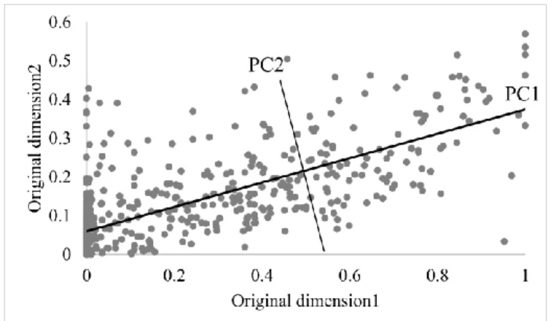
popularity. The principal component analysis (PCA) is one of the widely-used linear DR solutions. It is a non-targeting linear DR algorithm and can be applied to various datasets without complex modification. PCA was first proposed by Pearson in 1901 and has experienced several modifications to become the transformation we know today (Hotelling 1933, Wold 1968). PCA provides solutions to various multivariate problems, including data reduction and finding classes of similar objects (Wold, Esbensen and Geladi 1987). The multispectral or vector character of most remote sensing imagery enables it to transform the original spectral space to feature spaces constructed by new components (Richards and Richards 1999). The PCA is a statistical procedure that uses orthogonal transformation to convert a set of observations of possibly correlated variables into a set of values of linearly uncorrelated variables called principal components (PCs) (Figure 1-4).
Figure 1-4: Principal component analysis illustration.
Yet, the results from linear DR can fail to be optimal due to the nonlinear features lying in a lot of data. For example, to linearly project data that is on or near a curved low dimensional space onto a linear subspace will lead to a large error (e.g. Swiss roll dataset (Figure 1-5)), unless the subspace has a higher dimension than the original curved space, which contradicts the objective of DR (Kambhatla and Leen 1993). In light of this, more complex nonlinear DR algorithms that address the underlying nonlinear features in these data have been proposed (e.g. locally linear embedding (LLE) and Laplacian eigenmaps (LE)). The nonlinear DR implies that the linear DR only focuses on preserving the
straight-line Euclidean distance of the data and neglects the nonlinear structure in the data (Zhang and Zha 2004). Two streams of nonlinear DR algorithms are based on geodesic distances and local structures, respectively. The first stream of nonlinear DR algorithms uses the geodesic distance to reveal the true data structure (Tenenbaum, De Silva and Langford 2000). The second stream of nonlinear DR algorithms maintains the local nonlinear structure during any transformation (Hastie and Stuetzle 1989).
Figure 1-5: Swiss roll dataset illustration:
(a) original Swiss roll dataset; dimension-reduced result from (b) PCA (principle component analysis); (c) LLE (locally linear embedding); and (d) LE (Laplacian
eigenmaps).
1.4.4
Multilinear algebra notation and preliminaries
The above descriptions of the two hyperspectral image processing methods (SMA (spectral mixture analysis) and DR (dimension reduction)) both have the potential to benefit from the current trend of multilinear algebra. Before introducing how to apply multilinear algebra in SMA and DR, I will first provide the basic concepts of multilinear algebra. In mathematics, an Nth-order tensor is a N-dimensional array: 𝓧 ∈ ℝ𝐼1×𝐼2×⋯×𝐼𝑁.
In simple cases, a vector is a first-order tensor, a matrix is a second-order tensor, and a data cube (e.g. a hyperspectral image) is a third-order tensor. The order of a tensor is the
number of dimensions, which can be also called ways or modes. In this thesis, I maintained the widely used notations among mathematical articles. Vectors (first-order tensor) are denoted by boldface lowercase letters, e.g. a, and their ith entry is denoted by 𝑎𝑖. Matrices (second-order tensor) are denoted by boldface capital letters, e.g., A, and
their element (𝑖, 𝑗) is denoted by 𝑎𝑖𝑗. Third-order or higher-order tensors are denoted by
boldface Euler script letters, e.g. 𝓧, and elements (𝑖, 𝑗, 𝑘) of a third-order tensor are denoted by 𝑎𝑖𝑗𝑘. Subscript indices range from 1 to their capital versions, e.g., 𝑖 = 1, ⋯ , 𝐼. The nth element in a sequence is denoted by a superscript in parentheses, e.g., 𝓧(𝑛) denotes the nth tensor in a sequence. Subarrays are derived from fixing a subset of index. A colon is used to denote all elements of a mode. In the case of matrices, the subarrays are rows (𝑎𝑖:) and columns (𝑎:𝑗). For higher-order tensors, the subarrays are called fibers when fixing all but one indices or called slices when fixing all but two indices (Figure 1-6).
Figure 1-6: Fibers and slices of a third-order tensor:
(a) Mode-1 fibers 𝒂:𝒋𝒌; (b) Mode-2 fibers 𝒂𝒊:𝒌; (c) Mode-3 fibers 𝒂𝒊𝒋:; (d) Horizontal slices 𝑿𝒊∷; (e) Lateral slices 𝑿:𝒋:; and (f) Frontal slices 𝑿∷𝒌 (Kolda and Bader 2009).
Unfolding is another basic transformation of a tensor, and is also referred to as matricization and flattening. The unfolding process reorders the elements of a tensor into a matrix, which is a step required by certain analyses. There are many ways to assemble the elements from a tensor into a matrix. This thesis only applied the mode-𝑛 unfolding, denoted by X(n). The mode-n unfolding takes the mode-n fibers as columns in the
resulting matrix.
Analogous to the matrix Frobenius norm denoted as ∥ 𝐴 ∥, the norm of a tensor 𝒳 ∈ ℝ𝐼1×𝐼2×⋯×𝐼𝑁 is the square root of the sum of the squares of all its elements:
∥ 𝒳 ∥= √∑ ∑𝐼2 ⋯ 𝑖2=1 𝐼1 𝑖1=1 ∑ 𝑥𝑖1𝑖2⋯𝑖𝑁 2 𝐼𝑁 𝑖𝑁=1 , (1-1)
Tensors can be multiplied by matrices using the n-mode product. It is a basic tensor calculation that is used in tensor-based multilinear operations. The n-mode product multiplies a tensor 𝒳 ∈ ℝI1×⋯×In×⋯×IN by a matrix U ∈ ℝJ×In in mode n, and is denoted
by 𝒳 ×𝑛𝑈. The product result has a size of 𝐼1 × ⋯ 𝐼1× ⋯ × 𝐼𝑛−1× 𝐽 × 𝐼𝑛+1× ⋯ × 𝐼𝑁.
The element of the result is calculated as below:
(𝒳 ×𝑛𝑈)𝑖1⋯𝑖𝑛−1𝑗𝑖𝑛+1⋯𝑖𝑁 = ∑𝐼𝑛 𝑥𝑖1𝑖2⋯𝑖𝑁𝑢𝑗𝑖𝑛
𝑖𝑛=1 , (1-2)
The n-mode product can be also interpreted as multiplying each mode-n fiber with the matrix:
𝒴 = 𝒳 ×𝑛𝑈 ⟺ 𝑌(𝑛) = 𝑈𝑋𝑛 (1-3)
In order to explore the hidden information in a tensor, different tensor decomposition methods have been proposed to deal with different problems. Two main tensor decomposition methods include CANDECOMP/PARAFAC (CP) decomposition and Tucker decomposition. Hitchcock proposed the initial idea of CP decomposition in 1927 (Hitchcock 1927). CP decomposition did not become popular until 1970 when Carroll and Chang re-introduced the concept of CANDECOMP (canonical decomposition) (Carroll and Chang 1970) and Harshman re-introduced the concept of PARAFAC (parallel factors) (Harshman 1970) in the psychometrics community. The CP decomposition adopts a polyadic form, expressing a tensor as the sum of a finite number
of rank-one tensors (Figure 1-7). A rank-one tensor 𝒳 ∈ ℝ𝐼1×𝐼2×⋯×𝐼𝑁 is an Nth-order
tensor that can be obtained from the outer product of N vectors. The outer product is the tensor product of two coordinate vectors. Given two tensors 𝒜 ∈ ℝ𝐼1×𝐼2…×𝐼𝑝 and ℬ ∈
ℝ𝐽1×𝐽2…×𝐽𝑄, the outer product is written as 𝒜 ∘ ℬ ∈ ℝ𝐼1×𝐼2…×𝐼𝑝×𝐽1×𝐽2…×𝐽𝑄. The element is
obtained as below:
(𝒜 ∘ ℬ)𝑖1𝑖2…𝑖𝑃𝑗1𝑗2…𝑗𝑄 = 𝑎𝑖1𝑖2…𝑖𝑃𝑏𝑗1𝑗2…𝑗𝑄, (1-4)
The CP decomposition for a third-order tensor 𝒳 ∈ ℝ𝐼×𝐽×𝐾 can be written as:
𝒳 ≈ ∑𝑅𝑟=1𝑎𝑟°𝑏𝑟°𝑐𝑟, (1-5)
where R is the number of dimensions of 𝒳. The smallest R that fulfills the Equation (1-5) is the rank of a tensor. Unfortunately, there is no straightforward way to determine the rank of a tensor.
The Tucker decomposition was first proposed by Tucker in 1963 (Tucker 1963) (Figure 1-7). It decomposes a tensor into a core tensor multiplied by a matrix along each mode:
𝒳 ≈ 𝒢 ×1𝐴 ×2 𝐵 ×3𝐶, (1-6)
The size of the core 𝒢 is the key input in Tucker decompositions, which is not readily available but is obtained through experiments.
Figure 1-7: Tensor decomposition illustration:
(a) CP (CANDECOMP/PARAFAC) decomposition; (b) Tucker decomposition.
As the majority of current image processing methods are based on 2D matrix calculation, the hyperspectral 3D cube needs to be matricized in order to be processed, which discards the spatial information along the two spatial dimensions. The above-introduced multilinear algebra enables the direct calculation between 3D cubes that are referred to as 3D tensors. Thus, the tensor-based image processing method preserves the spatial information in the original image.
1.5
Organization of the thesis
The thesis consists of five chapters. Chapter 1 provides the research context, explains the thesis objectives, states the major research questions, and provides the necessary background. Chapters 2-4 separately covers:
(1) Evaluation of SMA methods for simulated EnMAP hyperspectral imagery.
(3) The application of spectral-spatial representation of hyperspectral images in DR.
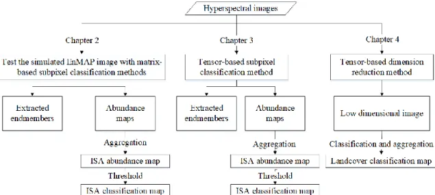
Chapter 2 concerns the application of the future EnMAP image in ISA mapping. Chapter 3 concerns the application of the multilinear algebra in spectral unmixing for ISA mapping using hyperspectral images. Chapter 4 concerns the application of the multilinear algebra in dimension reduction for land cover mapping using hyperspectral images. Figure 1-8 shows the relations between Chapters 2-4. The ultimate achievement of them is to obtain accurate and reliable ISA/land cover maps from hyperspectral images. Chapter 5 concludes the main findings from Chapters 2-4.
Figure 1-8: Relationship among the three sub-studies.
References
Anderson, J. R. 1976. A land use and land cover classification system for use with remote sensor data. US Government Printing Office.
Arnold Jr, C. L. & C. J. Gibbons (1996) Impervious surface coverage: the emergence of a key environmental indicator. Journal of the American planning Association, 62,
243-258.
Benediktsson, J. A., J. A. Palmason & J. R. Sveinsson (2005) Classification of
hyperspectral data from urban areas based on extended morphological profiles.
Bioucas-Dias, J. M., A. Plaza, G. Camps-Valls, P. Scheunders, N. M. Nasrabadi & J. Chanussot (2013) Hyperspectral remote sensing data analysis and future challenges. Geoscience and Remote Sensing Magazine, IEEE, 1, 6-36. Buckingham, R. & K. Staenz (2008) Review of current and planned civilian space
hyperspectral sensors for EO. Canadian Journal of Remote Sensing, 34, S187-S197.
Buyantuyev, A. & J. Wu (2010) Urban heat islands and landscape heterogeneity: linking spatiotemporal variations in surface temperatures to land-cover and
socioeconomic patterns. Landscape ecology, 25, 17-33.
Carlson, T. N. & S. T. Arthur (2000) The impact of land use—land cover changes due to urbanization on surface microclimate and hydrology: a satellite perspective.
Global and planetary change, 25, 49-65.
Carroll, J. D. & J.-J. Chang (1970) Analysis of individual differences in multidimensional scaling via an N-way generalization of “Eckart-Young” decomposition.
Psychometrika, 35, 283-319.
Chang, C.-I., C.-C. Wu, W.-m. Liu & Y.-C. Ouyang (2006) A new growing method for simplex-based endmember extraction algorithm. Geoscience and Remote Sensing, IEEE Transactions on, 44, 2804-2819.
Chen, J., J. Chen, A. Liao, X. Cao, L. Chen, X. Chen, C. He, G. Han, S. Peng & M. Lu (2015) Global land cover mapping at 30 m resolution: A POK-based operational approach. ISPRS Journal of Photogrammetry and Remote Sensing, 103, 7-27. Clark, R. N., G. A. Swayze, R. Wise, K. E. Livo, T. M. Hoefen, R. F. Kokaly & S. J.
Sutley. 2007. USGS digital spectral library splib06a. US Geological Survey Reston, VA.
Deng, C. & C. Wu (2013) A spatially adaptive spectral mixture analysis for mapping subpixel urban impervious surface distribution. Remote Sensing of Environment,
133, 62-70.
Dozier, J. (1981) A method for satellite identification of surface temperature fields of subpixel resolution. Remote Sensing of environment, 11, 221-229.
Fan, F., W. Fan & Q. Weng (2015) Improving urban impervious surface mapping by linear spectral mixture analysis and using spectral indices. Canadian Journal of Remote Sensing, 41, 577-586.
Fauvel, M., J. A. Benediktsson, J. Chanussot & J. R. Sveinsson (2008) Spectral and spatial classification of hyperspectral data using SVMs and morphological profiles. Geoscience and Remote Sensing, IEEE Transactions on, 46, 3804-3814.
Gao, F., E. B. de Colstoun, R. Ma, Q. Weng, J. G. Masek, J. Chen, Y. Pan & C. Song (2012) Mapping impervious surface expansion using medium-resolution satellite image time series: a case study in the Yangtze River Delta, China. International Journal of Remote Sensing, 33, 7609-7628.
Harshman, R. A. (1970) Foundations of the PARAFAC procedure: Models and conditions for an" explanatory" multimodal factor analysis.
Hastie, T. & W. Stuetzle (1989) Principal curves. Journal of the American Statistical Association, 84, 502-516.
Hitchcock, F. L. (1927) The expression of a tensor or a polyadic as a sum of products.
Studies in Applied Mathematics, 6, 164-189.
Hotelling, H. (1933) Analysis of a complex of statistical variables into principal components. Journal of educational psychology, 24, 417.
Hu, X. & Q. Weng (2011) Impervious surface area extraction from IKONOS imagery using an object-based fuzzy method. Geocarto International, 26, 3-20.
Huang, X. & L. Zhang (2009) A comparative study of spatial approaches for urban mapping using hyperspectral ROSIS images over Pavia City, northern Italy.
International Journal of Remote Sensing, 30, 3205-3221.
Kambhatla, N. & T. K. Leen. 1993. Fast nonlinear dimension reduction. In Neural Networks, 1993., IEEE International Conference on, 1213-1218. IEEE. Karn, S. K. & H. Harada (2001) Surface water pollution in three urban territories of
Nepal, India, and Bangladesh. Environmental Management, 28, 483-496. Kolda, T. G. & B. W. Bader (2009) Tensor decompositions and applications. SIAM
review, 51, 455-500.
Leopold, L. B. (1968) Hydrology for urban land planning: A guidebook on the hydrologic effects of urban land use.
Li, H., L. J. Sharkey, W. F. Hunt & A. P. Davis (2009) Mitigation of impervious surface hydrology using bioretention in North Carolina and Maryland. Journal of
Hydrologic Engineering, 14, 407-415.
Liu, W., K. C. Seto, E. Y. Wu, S. Gopal & C. E. Woodcock (2004) ART-MMAP: A neural network approach to subpixel classification. Geoscience and Remote Sensing, IEEE Transactions on, 42, 1976-1983.
Loperfido, J. V., G. B. Noe, S. T. Jarnagin & D. M. Hogan (2014) Effects of distributed and centralized stormwater best management practices and land cover on urban stream hydrology at the catchment scale. Journal of Hydrology, 519, 2584-2595.
Lu, D., S. Hetrick & E. Moran (2011a) Impervious surface mapping with Quickbird imagery. International journal of remote sensing, 32, 2519-2533.
Lu, D., G. Li, W. Kuang & E. Moran (2014) Methods to extract impervious surface areas from satellite images. International Journal of Digital Earth, 7, 93-112.
Lu, D., G. Li, E. Moran, M. Batistella & C. C. Freitas (2011b) Mapping impervious surfaces with the integrated use of Landsat Thematic Mapper and radar data: A case study in an urban–rural landscape in the Brazilian Amazon. ISPRS Journal of Photogrammetry and Remote Sensing, 66, 798-808.
Lu, D., E. Moran & S. Hetrick (2011c) Detection of impervious surface change with multitemporal Landsat images in an urban–rural frontier. ISPRS Journal of Photogrammetry and Remote Sensing, 66, 298-306.
McKinney, M. L. (2008) Effects of urbanization on species richness: a review of plants and animals. Urban ecosystems, 11, 161-176.
Miller, J. D., H. Kim, T. R. Kjeldsen, J. Packman, S. Grebby & R. Dearden (2014) Assessing the impact of urbanization on storm runoff in a peri-urban catchment using historical change in impervious cover. Journal of Hydrology, 515, 59-70. Momeni, R., P. Aplin & D. S. Boyd (2016) Mapping complex urban land cover from
spaceborne imagery: the influence of spatial resolution, spectral band set and classification approach. Remote Sensing, 8, 88.
Paul, M. J. & J. L. Meyer (2001) Streams in the urban landscape. Annual Review of Ecology and Systematics, 333-365.
Pauleit, S., R. Ennos & Y. Golding (2005) Modeling the environmental impacts of urban land use and land cover change—a study in Merseyside, UK. Landscape and urban planning, 71, 295-310.
Plaza, A., P. Martínez, R. Pérez & J. Plaza (2004) A quantitative and comparative
analysis of endmember extraction algorithms from hyperspectral data. Geoscience and Remote Sensing, IEEE Transactions on, 42, 650-663.
Powell, R. L., D. A. Roberts, P. E. Dennison & L. L. Hess (2007) Sub-pixel mapping of urban land cover using multiple endmember spectral mixture analysis: Manaus, Brazil. Remote Sensing of Environment, 106, 253-267.
Richards, J. A. & J. Richards. 1999. Remote sensing digital image analysis. Springer. Roberts, D. A., M. Gardner, R. Church, S. Ustin, G. Scheer & R. Green (1998) Mapping
chaparral in the Santa Monica Mountains using multiple endmember spectral mixture models. Remote Sensing of Environment, 65, 267-279.
Schneider, A., M. A. Friedl & D. Potere (2010) Mapping global urban areas using MODIS 500-m data: New methods and datasets based on ‘urban ecoregions’.
Remote Sensing of Environment, 114, 1733-1746.
Seto, K. C., B. Güneralp & L. R. Hutyra (2012) Global forecasts of urban expansion to 2030 and direct impacts on biodiversity and carbon pools. Proceedings of the National Academy of Sciences, 109, 16083-16088.
Sung, C. Y. & M.-H. Li (2012) Considering plant phenology for improving the accuracy of urban impervious surface mapping in a subtropical climate regions.
International journal of remote sensing, 33, 261-275.
Tenenbaum, J. B., V. De Silva & J. C. Langford (2000) A global geometric framework for nonlinear dimensionality reduction. Science, 290, 2319-2323.
Tucker, L. R. (1963) Implications of factor analysis of three-way matrices for measurement of change. Problems in measuring change, 15, 122-137. Vagni, F. (2007) Survey of hyperspectral and multispectral imaging technologies.
Van der Meer, F. D., H. M. A. Van der Werff, F. J. Van Ruitenbeek, C. A. Hecker, W. H. Bakker, M. F. Noomen, M. Van Der Meijde, E. J. M. Carranza, J. B. De Smeth & T. Woldai (2012) Multi-and hyperspectral geologic remote sensing: A review.
International Journal of Applied Earth Observation and Geoinformation, 14, 112-128.
Voogt, J. A. & T. R. Oke (2003) Thermal remote sensing of urban climates. Remote sensing of environment, 86, 370-384.
Weng, Q., X. Hu & D. Lu (2008) Extracting impervious surfaces from medium spatial resolution multispectral and hyperspectral imagery: a comparison. International Journal of Remote Sensing, 29, 3209-3232.
Wickham, J. D., S. V. Stehman, L. Gass, J. Dewitz, J. A. Fry & T. G. Wade (2013) Accuracy assessment of NLCD 2006 land cover and impervious surface. Remote Sensing of Environment, 130, 294-304.
Wolch, J. R., J. Byrne & J. P. Newell (2014) Urban green space, public health, and environmental justice: The challenge of making cities ‘just green enough’.
Landscape and Urban Planning, 125, 234-244.
Wold, H. O. A. 1968. Nonlinear estimation by iterative least square procedures.
Wold, S., K. Esbensen & P. Geladi (1987) Principal component analysis. Chemometrics and intelligent laboratory systems, 2, 37-52.
Wu, C. & A. T. Murray (2003) Estimating impervious surface distribution by spectral mixture analysis. Remote sensing of Environment, 84, 493-505.
Xian, G. & M. Crane (2006) An analysis of urban thermal characteristics and associated land cover in Tampa Bay and Las Vegas using Landsat satellite data. Remote Sensing of environment, 104, 147-156.
Xu, H. (2010) Analysis of impervious surface and its impact on urban heat environment using the normalized difference impervious surface index (NDISI).
Photogrammetric Engineering & Remote Sensing, 76, 557-565.
Yang, F., B. Matsushita & T. Fukushima (2010) A pre-screened and normalized multiple endmember spectral mixture analysis for mapping impervious surface area in Lake Kasumigaura Basin, Japan. ISPRS Journal of Photogrammetry and Remote Sensing, 65, 479-490.
Yuan, F. & M. E. Bauer (2007) Comparison of impervious surface area and normalized difference vegetation index as indicators of surface urban heat island effects in Landsat imagery. Remote sensing of Environment, 106, 375-386.
Zhang, L., Q. Weng & Z. Shao (2017) An evaluation of monthly impervious surface dynamics by fusing Landsat and MODIS time series in the Pearl River Delta, China, from 2000 to 2015. Remote Sensing of Environment, 201, 99-114. Zhang, Z.-y. & H.-y. Zha (2004) Principal manifolds and nonlinear dimensionality
reduction via tangent space alignment. Journal of Shanghai University (English Edition), 8, 406-424.
Zhou, W., Y. Qian, X. Li, W. Li & L. Han (2014) Relationships between land cover and the surface urban heat island: seasonal variability and effects of spatial and thematic resolution of land cover data on predicting land surface temperatures.
Landscape ecology, 29, 153-167.
Zhuo, L., B. Cheng & J. Zhang (2014) A comparative study of dimensionality reduction methods for large-scale image retrieval. Neurocomputing, 141, 202-210.
2
Evaluation of unmixing methods for simulated EnMAP hyperspectral
imagery
The distribution of impervious surface area (ISA) is an important input in a wide range of urban ecosystem studies, including urban hydrology, urban climate, land use planning, and resource management (Arnold Jr and Gibbons 1996, Voogt and Oke 2003, McKinney 2008, Wolch, Byrne and Newell 2014). Remote sensing has been playing a key role in ISA mapping. To date, the majority of ISA mapping literatures used multispectral sensors, for example MODIS, Landsat ETM+, and QuickBird, etc. Thus, more efforts have been oriented to spatial heterogeneity and much less effort has been devoted to spectral diversity (Weng 2012). It may due to the lack of economic, timely, and global hyperspectral data. The future launch of EnMAP (Environmental mapping and Analysis Program) hyperspectral satellite in 2019 provides new opportunities for ISA mapping (Kaufmann et al. 2006, Guanter et al. 2015). Although hyperspectral sensors have been studied for more than three decades, most mature hyperspectral sensors are mounted on airplanes: FLI and CASI (Gower et al. 1992), AVIRIS (Vane et al. 1993), Hydice (Rickard et al. 1993), HyMap (Cocks et al. 1998), etc. The only three active hyperspectral satellites are NASA’s Hyperion (Pearlman et al. 2003), NASA’s HICO (Corson et al. 2008), and ESA’s CHRIS (Barnsley et al. 2004). However, the CHRIS and HICO are limited to the visible to near-infrared (VNIR) region (400-1400 nm), and Hyperion has a low signal-to-noise ratio, which limits its feature detection capabilities. Therefore, the EnMAP mission is a milestone towards a comprehensive hyperspectral observation from space (Guanter et al. 2015). The designed EnMAP hyperspectral sensor has a 30 m spatial resolution and its spectral range is between 420 and 2450 nm with a spectral sampling distance varying between 5 and 12 nm. The global revisit capability of EnMAP hyperspectral satellite is 21 days. The potential of using EnMAP images in urban environments has been extensively discussed by Heldens et al, 2011, and ISA mapping has been recognized as one of the great strengths of the EnMAP hyperspectral sensor (Heldens et al. 2011).
2.1
Background
2.1.1
Previous studies on EnMAP
An EnMAP end-to-end simulation tool (EeteS) was designed by Segl et al. (Segl et al. 2012) for calibrating the fundamental instrument parameters, developing the data pre-processing steps, and evaluating the exploitable algorithms. The EeteS software simulates EnMAP images using reflectance data that has spectrally and spatially oversampled resolution than the EnMAP final sampling interval. To date, 18 publications have used the simulated EnMAP images for various earth observation applications (Braun, Weidner and Hinz 2012, Okujeni, van der Linden and Hostert 2015, Rogge et al. 2014, Schwieder et al. 2014, Suess et al. 2015, Yokoya, Chan and Segl 2016, Locherer et al. 2015, Marcinkowska-Ochtyra et al. 2017, Fassnacht, Weinacker and Koch 2011, Lehnert et al. 2014, Dotzler et al. 2015, Steinberg et al. 2016, Clasen et al. 2015, Malec et al. 2015, Leitão et al. 2015, Xi et al. 2015, Siegmann et al. 2015, Mielke et al. 2014) (Table 1), most of which target natural or agricultural environments and only one is in urban environments. In order to produce classification maps or predict certain geographic features, 14 of the publications used the endmembers or training samples obtained from other high-resolution images or existed reference data. Only four publications extracted endmembers directly from simulated EnMAP images, but they are large-scale studies in natural environments, where land cover changes less rapidly than in urban environment. The reason why we want to extract endmembers directly from remote sensing imagery is that field/lab reference data is acquired under different conditions from the airborne or spaceborne data and can cause errors in following analyses.
Table 2-1: Publications on the application of simulated EnMAP images.
Year Authors Applications Endmember extraction methods/ training sample sources
Methods
2017 Marcinkowska-Ochtyra, et. al.
Per-pixel vegetation classification in subalpine and alpine areas.
Field survey reference map and pixel purity index (PPI) from the airborne APEX images.
Support vector machines (SVM).
2016 Yokoya, et. al. Sub-pixel geologic material classification in temperate bare rock area.
Vertex component analysis (VCA) and visual inspection from reference image.
Coupled nonnegative matrix factorization (CNMF) fusion (Yokoya, Yairi and Iwasaki 2012) and multiple endmember SMA (MESMA) (Roberts et al. 1998b).
2016 Steinberg, et. al. Predict common surface soil properties
Ground truth measurements. Partial least squares regression (PLSR) (Oldenburg, Schmidtlein and Feilhauer).
2015 Okujeni, et. al. Sub-pixel land cover classification in urban-rural gradient area.
Reference spectral library from airborne HyMap images.
Support vector regression (SVR) (Okujeni et al. 2013).
2015 Suess, et. al. Per-/sub-pixel shrub cover abundance classification.
Manually selected from simulated EnMAP images.
Support vector classification (SVC) and adapted SVC (classification). 2015 Clasen, et. al. Sub-pixel forest crown
classification.
Field survey measurements. MESMA.
2015 Malec, et. al. Sub-pixel soil degradation cover abundance classification.
Extracted from the EnMAP image using updated spatial spectral endmember
extraction tool (SSEE) method (Rogge et al. 2012).
MESMA.
2015 Leitão, et. al. Predict shrub cover abundance classification.
Reference map. Boosted regression tree (BRT) (Elith, Leathwick and Hastie 2008). 2015 Locherer, et. al. Predict leaf area index (LAI)
during agriculture growing season.
Field survey measurements. Look-up-table based inversion of the PROSAIL model.
2015 Siegmann, et. al. Predict LAI in wheat field. Field survey measurements. Ehlers fusion and PLSR.
2015 Xi, et. al. Predict phytoplankton taxonomic groups
Lab measurements. Similarity index and hierarchical cluster analysis.
2015 Dotzler, et. al. Predict drought stress phenomena in deciduous forest communities.
Reference map. Analyses of variance (ANOVA), and Tukey’s HSD post-hoc tests using drought-sensitive spectral indices.
Year Authors Applications Endmember extraction methods/ training sample sources
Methods
2014 Rogge, et. al. Sub-pixel geologic material classification in subarctic bare rock area.
Extracted from the EnMAP image using updated SSEE method.
Iterative SMA (ISMA) (Rogge et al. 2006)
2014 Schwieder, et. al. Sub-pixel shrub cover abundance classification.
Reference map. SVR (Karatzoglou, Meyer and Hornik 2005), random forest regression (RF) (Liaw and Wiener 2002), and PLSR (Wehrens and Mevik 2007). 2014 Lehnert, et. al. Sub-pixel classification of
rangeland degradation in the Tibetan Plateau and predict chlorophyll content.
Field s