Kernel Flows:
from learning kernels from data into the abyss
Houman Owhadi∗and Gene Ryan Yoo†September 25, 2018
Abstract
Learning can be seen as approximating an unknown function by interpolating the training data. Kriging offers a solution to this problem based on the prior specification of a kernel. We explore a numerical approximation approach to kernel selection/construction based on the simple premise that a kernel must be good if the number of interpolation points can be halved without significant loss in accuracy (measured using the intrinsic RKHS normk · kassociated with the kernel). We first test and motivate this idea on a simple problem of recovering the Green’s function of an elliptic PDE (with inhomogeneous coefficients) from the sparse observation of one of its solutions. Next we consider the problem of learning non-parametric families of deep kernels of the formK1(Fn(x), Fn(x0)) with Fn+1 = (Id+Gn+1)◦Fn and
Gn+1 ∈span{K1(Fn(xi),·)}. With the proposed approach constructing the kernel becomes equivalent to integrating a stochastic data driven dynamical system, which allows for the training of very deep (bottomless) networks and the exploration of their properties. These networks learn by constructing flow maps in the kernel and input spaces via incremental data-dependent deformations/perturbations (appearing as the cooperative counterpart of adversarial examples) and, at profound depths, they (1) can achieve accurate classification from only one data point per class (2) appear to learn archetypes of each class (3) expand distances between points that are in different classes and contract distances between points in the same class.
For kernels parameterized by the weights of Convolutional Neural Networks, min-imizing approximation errors incurred by halving random subsets of interpolation points, appears to outperform training (the same CNN architecture) with relative entropy and dropout.
1
Introduction
Despite their popularity and impressive achievements [14] Artificial Neural Networks (ANNs) remain difficult to analyze. From a deep kernel learning perspective [35], the
∗
Corresponding author. California Institute of Technology, 1200 E California Blvd, MC 9-49, Pasadena, CA 91125, USA, [email protected]
†
California Institute of Technology, 1200 E California Blvd, MC 253-47, Pasadena, CA 91125, USA, [email protected]
action of the last layer of an ANN can be seen as that of regressing the data with a kernel parameterized by the weights of all the previous layers. Therefore analysing the problem of performing a regression of the data with a kernel that is also learnt from the data could help understand ANNs and elaborate a rigorous theory for deep learning. Hierarchical Bayesian Inference [29] (placing a prior on a space of kernels and conditioning on the data) and Maximum Likelihood Estimation [34] (choosing the kernel which maximizes the probability of observing the data) are well known approaches for learning the kernel. In this paper we explore a numerical approximation approach (motivated by interplays between Gaussian Process Regressions and Numerical Homogenization [21]) based on the simple premise that a kernel must be good if the number of points N used to perform the interpolation of data can be reduced to N/2 without significant loss in accuracy (measured using the intrinsic RKHS norm k · k associated with the kernel). Writing
u and v for the interpolation of the data with N and N/2 points, the relative error
ρ = kuk−ukv2k2 induces a data dependent ordering on the space of kernels. The Fr´echet
derivative of ρ identifies the direction of the gradient descent and leads to a simple algorithm (Kernel Flow) for its minimization: (1) Select Nf (≤N) points (at random, uniformly, without replacement) from theN training data points (2) SelectNc=Nf/2 points (at random, uniformly, without replacement) from theNf points (3) Perturb the kernel in the gradient descent direction ofρ (computed from the current kernel and the
Nf, Ncpoints) (4) Repeat.
To provide some context for this algorithm, we first summarize (in Section 2) in-terplays between Kriging, Gaussian Process Regression, Game Theory and Optimal Recovery. The identification (in Sec. 3) of ρ and its Fr´echet derivative leads (in Sec.4) to the proposed algorithm in a parametric setting.
In Sec. 5we describe interplays between the proposed algorithm and Numerical Ho-mogenization [21] by implementing and testing the parametric version of Kernel Flow for the (simple and amenable to analysis) problem of (1) recovering the unknown conduc-tivityaof the PDE−div(a∇u) =f based on seeingu∈ H1
0((0,1)) at a finite numberN of points (2) approximatingu between measurement points. For this problem,a,u and
f are all unknown, we only know thatf ∈L2 and we try to learn the Green’s function of the PDE (seen as a kernel parameterized by the unknown conductivitya). Experiments suggest that, by minimizing ρ (parameterized by the conductivity), the algorithm can recover the conductivity and significantly improve the accuracy of the interpolation.
Next (in Sec. 6) we derive a non parametric version of the proposed algorithm that learns a kernel of the form
Kn(x, x0) =K1(Fn(x), Fn(x0)), (1.1) where K1 is a standard kernel (e.g. GaussianK1(x, x0) =e−γ|x−x
0|2
) and Fn maps the input space into itself,n→Fnis a discrete flow in the input space, andFn+1 is obtained from Fn by interrogating random subsets of the training data as described in Fig. 1
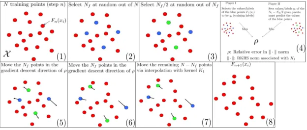
Figure 1: The game theoretic interpretation of the stepn→ n+ 1 of Kernel Flow. (1) Starting from Fn and the N data points (Fn(xi), yi) (2) Select Nf indices out of N (3) SelectNf/2 indices out ofNf (4) Consider the zero sum adversarial game where Player I chooses the labels of theNf points to be yi and Player II sees half of them and tries to guess the other and let ρ be the loss of Player II in that game (using relative error in the RKHS norm associated with K1) (5, 6) Move the Nf selected points Fn(xi) to decrease the loss of Player II (7) Move the remaining N −Nf (and any other point x) points via interpolation with the kernelK1 (this specifies Fn+1) (8) Repeat.
(which also summarizes the game theoretic interpretation of the proposed Algorithm, note that the game is incrementally rigged to minimize the loss of Player II).
The proposed algorithm (see Fig. 2 for a summary of its structure) can be reduced to an iteration of the form
Kn(x, x0) =Kn−1(x+Gn(x), x+Gn(x0)). (1.2) Writingxi for the training points andF1(x) =x and Fn(x) = (Id+Gn)◦Fn−1(x), the networkFn (composed ofnlayers) is learnt from the data in a recursive manner (across layers) by (1) usinggi(n):=Gn◦Fn−1(xsf,n(i)) for a random subset{xsf,n(i)|1≤i≤Nf} of the points{xi|1≤i≤N}as training parameters and interpolatingGnwith the kernel
K1 in between the pointsFn−1(xsf,n(i)) (2) selectingg (n)
i in the direction of the gradient descent ofρ at each step.
Writing (xi, yi) for theN training data points, Gn+1 ends up being of the form
Gn+1(x) = Nf X
i=1
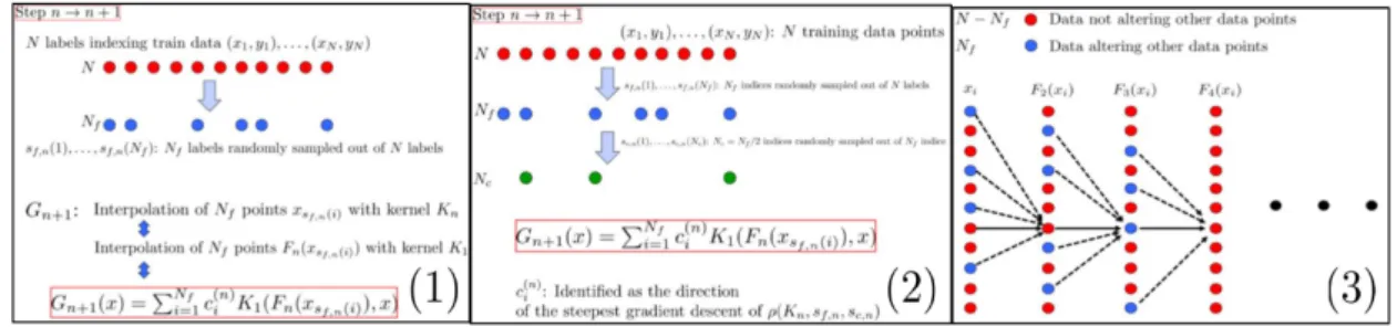
Figure 2: The Kernel Flow Algorithm. (1)Nf indicessf,n(1), . . . , sf,n(Nf) are randomly sampled out of N and Gn+1 belongs to the linear span of the K(F(x(snf,n() i)), x) (2) the coefficients in the representation of Gn+1 are found as the direction of the gradient de-scent ofρ (3) The value ofFn+1(xi) is the sum ofFn(xi) a small perturbation depending on the joint values of the Fn(xsf,n(j)).
where sf,n(1), . . . , sf,n(Nf) are Nf indices sampled at random (uniformly without re-placement) from{1, . . . , N}. Note that the kernelKn produced at any stepn, is a Deep Hierarchical Kernel (in the sense of [35,31]) satisfying the nesting equations
Kn(x, x0) =Kn−1(x+ Nf X i=1 c(in−1)Kn−1(xsf,n−1(i), x), x 0+ Nf X i=1 c(in−1)Kn−1(xsf,n−1(i), x 0)). (1.4) Furthermore, the structure of the network defined by that kernel is randomized through the random selection of the Nf points (see Fig. 2.3). The coefficients c(in) in (1.3) are identified through one step of gradient descent of the relative error ρ (measured in the RKHS norm associated withK1) of the approximation of the labels (theysf,n(i)) of those
Nf points upon seeing half of them. From the game theoretic perspective of Fig.1,ρ is the loss of Player II (attempting the guess the unseen labels) and the pointsFn+1(xsf,n(i)) are perturbations of the points Fn(xsf,n(i)) in a direction which seeks to minimize this loss. Note also that the proposed (Kernel Flow) algorithm produces a flow Fn (ran-domized through sampling of the training data) in the input space and a (stochastic) dynamical systemK1(Fn(x), Fn(y)) in the kernel space. Since learning becomes equiva-lent to integrating a dynamical system, it does not require back-propagation nor guessing the architecture of the network, which enables the construction of very deep networks and the exploration of their properties.
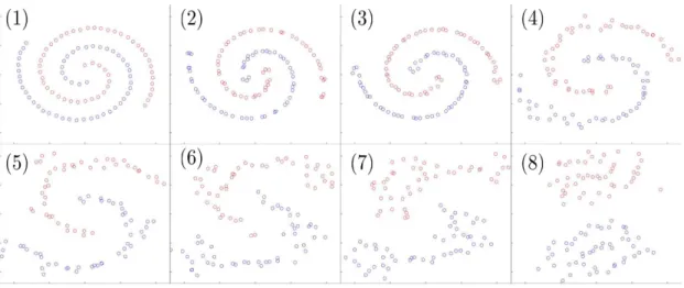
We implement this algorithm (and visualize its flow) for MNIST [37], Fashion-MNIST [36], the Swiss Roll Cheesecake. See Fig.3 and Fig.4for illustrations of the flow Fn(x) for the Swiss Roll Cheesecake and Fashion-MNIST. For these datasets we observe that (1) the flow Fn unrolls the Swiss Roll Cheesecake (2) the flow Fn expands distances between points that are in different classes and contracts distances between points in the same class (towards archetypes of each class) (3) at profound depths (n = 12000
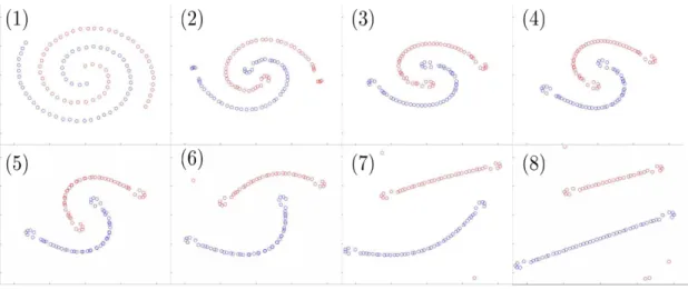
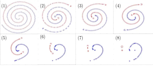
Figure 3: Swiss Roll Cheesecake. N = 100. Red points have label −1 and blue points have label 1. Fn(xi) for 8 different values ofn.
layers for MNIST and n = 50000 layers for Fashion-MNIST) the resulting kernel Kn achieves a small average error (1.5% for MNIST and 10% for Fashion-MNIST) using only 10 points as interpolation points (i.e. one point for each class) (4) the incremental data-dependent perturbationsGn+1seem to take advantage of a cooperative mechanism appearing as the counterpart of the one associated with adversarial examples [32,23].
Finally (in Sec. 10) we derive an ANN version of the algorithm by identifying the action of the last layer of the ANN as that of regressing the data with a kernel parame-terized by the weights of all the previous layers (learnt by minimizingρ or its analogous
L2 version). This algorithm is then tested for the MNIST and Fashion-MNIST data sets and shown to contract in-class distances and inter-class distances in a similar manner as above (thereby achieving accuracies comparable to the state of the art with a small number of interpolation points). For kernels parameterized by the weights of a given Convolutional Neural Network, minimizingρ or its L2 version, appears, for the MNIST and fashion MNIST data sets, to outperform training (the same CNN architecture) with relative entropy and dropout.
This paper is not aimed at identifying the state of the art algorithm in terms of accuracy nor complexity. It is simply motivated by an attempt to offer some insights (from a numerical approximation perspective) on mechanisms that may be at play in deep learning.
2
Learning as an interpolation problem
It is well understood [27] that “learning techniques are similar to fitting a multivariate function to a certain number of measurement data”, e.g. solving the following problem.
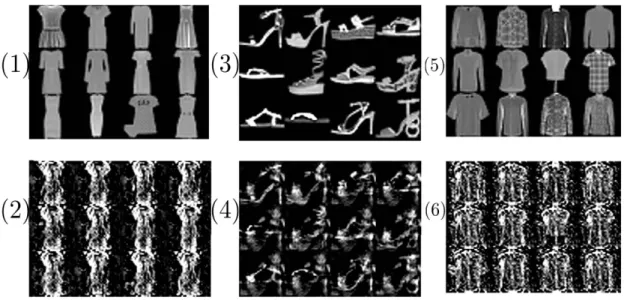
Figure 4: Results for Fashion-MNIST. N = 60000, Nf = 600 andNc = 300. (1, 3, 5) Training dataxi (class 3, 5 and 6) (2, 4, 6)Fn(xi) (class 3, 4 and 6) forn= 50000.
Problem 1. Given input/output data(x1, y1), . . . ,(xN, yN)∈ X ×Y recover an unknown
functionu† mapping X to Y such that
u†(xi) =yi for i∈ {1, . . . , N}. (2.1)
Optimal recovery. In the setting of optimal recovery [16] the ill posed problem 1
can be turned into a well posed one by restricting candidates for uto belong to a space of functions B endowed with a norm k · k and identifying the optimal recovery as the minimizer of the relative error
min v maxu
ku−vk2
kuk2 , (2.2)
where the max is taken over u∈ B and the min is taken over candidates in v ∈ B such that v(xi) = u(xi). Observe that B∗, the dual space of B, must contain delta Dirac functions
φi(·) :=δ(· −xi). (2.3) for the validity of the constraints u(xi) = yi. Consider now the case where k · k is quadratic, i.e. such that
kuk2= [Q−1u, u], (2.4)
where [φ, u] stands for the duality product between φ∈ B∗ and u∈ B and Q : B∗ → B
forϕ, φ∈ B∗). In that case the optimal solution of (2.2) has the explicit form (writing yi for u(xi)) v†= N X i,j=1 yiAi,jQφj, (2.5)
where A = Θ−1 and Θ is the N ×N Gram matrix with entries Θi,j = [φi, Qφj]. Fur-thermorev†can also be identified as the minimizer of
(
Minimize kψk
Subject to ψ∈ B and [φi, ψ] =yi, i∈ {1, . . . , N}.
(2.6)
Kriging. DefiningK as the kernel
K(x, x0) = [δ(· −x), Qδ(· −x0)], (2.7) (B,k · k) can be seen as a Reproducing Kernel Hilbert Space endowed with the norm
kuk2 = sup φ∈B∗
(Rφ(x)u(x)dx)2 R
φ(x)K(x, y)φ(y)dx dy , (2.8)
and (2.5) corresponds to the classical representer theorem
v†(·) =yTAK(x.,·), (2.9) using the vectorial notations yTAK(x.,·) = PNi,j=1yiAi,jK(xj,·) with A = Θ−1 and Θi,j =K(xi, xj).
Gaussian Process Regression numerical approximation games. Writingξ for the centered Gaussian Process with covariance function K, (2.9) can also be recovered via Gaussian Process Regression as
v†(x) =Eξ(x)|ξ(xi) =yi
. (2.10)
This link between Numerical Approximation and Gaussian Process Regression emerges naturally by viewing (2.2) as an adversarial zero sum game [21,18,20,28] between two players (I and II where I tries to maximize the relative error and II tries to minimize it after seeing the values of u at the pointsxi) and observing that ξ and v are optimal mixed/randomized strategies for players I and II (forming a saddle point for the minimax lifted to measures over functions).
3
What is a good kernel?
Although the optimal recovery ofu† has a well established theory, it relies on the prior specification of a quadratic normk · k or equivalently of a kernel K. In practical appli-cations the performance of the interpolant (2.9) (e.g. when employed in a classification
problem) is sensitive to the choice ofK. How should K be selected to achieve general-ization? Although ANNs [14] seem to address this question (by performing variants of the interpolation (2.9) with the last layer of the network using a kernelK parameterized by the weights of the previous layers and learnt by adjusting those weights) they remain difficult to analyze and the introduction of regularization steps (such as dropout or early stop) introduced to achieve generalization appear to be discovered through a laborious process of trial and error [38].
Is there a systematic way of identifying a good kernel? What is good kernel? We will now explore these questions from the perspective of interplays between nu-merical approximation and inference [21] and the simple premise that a kernel must be good if the number of pointsN used to perform the interpolation of data can be reduced to m = round(N/2) without significant loss in accuracy (measured using the intrinsic RKHS norm associated with the kernel).
To label the m sub-sampled (test) data points, let s(1), . . . , s(m) be a selection of
m distinct elements of {1. . . , N}. Observe that {xs(1), . . . , xs(m)} forms a strict subset of {x1, . . . , xN}. Write vs for the optimal recovery of u† upon seeing its values at the points xs(1), . . . , xs(m), and observe that vs(·) =
Pm
i=1y¯iA¯i,jK(xs(j), i) with ¯yi = ys(i) and ¯A = ¯Θ−1 with ¯Θi,j = Θs(i),s(j). Let π be the corresponding m×N sub-sampling matrix defined byπi,j =δs(i),j and observe that
vs =yTAK˜ (x.,·) (3.1) with ˜A=πTAπ¯ and ¯A= (πΘπT)−1.
Proposition 3.1. For v† and vs defined as in (2.9) and (3.1), we have
kv†−vsk2 =yTAy−yTAy .˜ (3.2) Proof. Proposition 3.1 is particular case of [21, Prop. 13.29]. The proof follows simply from kv†k2 =yTAy, kvsk2 = ¯yTA¯y¯=yTAy˜ and the orthogonal decomposition kv†k2 =
kvsk2 +kv†−vsk2 implied by the fact that vs is the minimizer of kψk2 subject to the constraints [φs(i), ψ] =ys(i) and thatv† satisfies those constraints.
Let ρ be the ratio
ρ:= kv
†−vsk2
kv†k2 . (3.3)
Note that a value ofρ close to zero indicates thatvs is a good approximation ofv†(and that most of the energy of v† is contained in vs) which is a desirable condition for the kernelK to achieve generalization. Furthermore, Prop.3.1implies thatρ∈[0,1] and
ρ= 1−y
TAy˜
yTAy. (3.4)
Fixingyandπ,ρcan be seen as a function ofAwhich we will writeρ(A). SinceA= Θ−1,
Motivating by the application of ρ to the ordering of space of kernels (a small ρ being indicative of a good kernel) we will, in the following proposition, compute its Fr´echet derivative with respect to small perturbations ofA or of Θ.
Proposition 3.2. Write z :=A−1Ay˜ with A˜:=πT(πA−1πT)−1π defined as above.1 It holds true that
ρ(A+S) =ρ(A) +(1−ρ(A))y
TSy−zTSz
yTAy +O(
2), (3.5)
and, writing2 yˆ:= Θ−1y and zˆ:=πT(πΘπT)−1πy,
ρ(Θ +T) =ρ(Θ)−(1−ρ(Θ))ˆy
TTyˆ−zˆTTzˆ ˆ
yTΘˆy +O(
2). (3.6)
Proof. Observe that
ρ(A+S) = 1−y
TπT(π(A+S)−1πT)−1πy
yT(A+S)y (3.7)
and recall the approximation
(A+S)−1 =A−1−A−1SA−1+O(2). (3.8) (3.5) then follows from straightforward calculus. The proof of (3.6) is identical and can also be obtained from (3.5) and the first order approximation (Θ +T)−1 = Θ−1 −
Θ−1TΘ−1+O(2).
4
The algorithm with a parametric family of kernels
Let W be a finite dimensional linear space and let K(x, x0, W) be a family of kernels parameterized by W ∈ W. LetNf ≤N and Nc = round(Nf/2). Let sf(1), . . . , sf(Nf) be a selection ofNf distinct elements of{1, . . . , N}. Letsc(1), . . . , sc(Nc) be a selection of
Nc distinct elements of {1, . . . , Nf}. Letπ be the corresponding Nc×Nf sub-sampling matrix defined by πi,j = δsc(i),j. Let yf ∈ RNf and yc ∈ RNc be the corresponding
subvectors ofy defined by yf,i=ysf(i) and yc,i =yf,sc(i).
Using the notations of sections 2 and 3 write Θ(W) for the Nf ×Nf matrix with entries Θi,j =K(xsf(i), xsf(j), W) and let
ρ(W, sf, sc) := 1−
yTc(πΘπT)−1yc
yT fΘ−1yf
. (4.1)
The following corollary derived from Prop. 3.2allows us to compute the gradient of
ρ respect toW.
1
The operatorP := ˜AA−1 is a projection with Im(P) = Im(πT) and Ker(P) =AKer(π) and from the perspective of numerical homogenization ˜Acan be interpreted as the homogenized version ofA[21, Sec. 13.10.3], see [21, Chap. 13.10] for further geometric properties.
Corollary 4.1. Write Θ := Θ(W), yˆ:= Θ−1yf and zˆ:= πT(πΘπT)−1πyf. Write Wi
for the entries of the vector W. It holds true that
∂Wiρ(W) =− (1−ρ(W))ˆyT(∂WiΘ(W))ˆy−zˆ T(∂ WiΘ(W))ˆz yT fΘ−1yf . (4.2)
Proof. Prop. 3.2implies that
ρ(W +W0) =ρ(W)−(1−ρ(W))ˆy
TTyˆ−zˆTTzˆ
yfTΘ−1yf
+O(2), (4.3)
withT = (W0)T∇WΘ(W), which proves the result.
The purpose of Algorithm 1 is to learn the parameters W (of the kernel K) from the data. The value of Nf (and hence Nc) corresponds to the size of a batch. The initialization ofW in step 1 may be problem dependent or at random.
Algorithm 1 LearningW in the K(·,·, W).
1: InitializeW 2: repeat 3: Selectsf(1), . . . , sf(Nf) out of {1, . . . , N}. 4: Selectsc(1), . . . , sc(Nc) out of {1, . . . , Nf}. 5: W0 =−∇Wρ(W, sf, sc) 6: W =W +W0
7: untilEnd criterion
5
A simple PDE model
To motivate, illustrate and study the proposed approach, it is useful to start with an application to the following simple PDE model amenable to detailed analysis [21]. Let
u be the solution of (
−div a(x)∇u(x)
=f(x) x∈Ω;
u= 0 on ∂Ω, (5.1)
where Ω⊂Rd, is a regular subset and ais a uniformly elliptic symmetric matrix with entries in L∞(Ω). Write L := −div(a∇·) for the corresponding linear bijection from
H1
0(Ω) toH−1(Ω).
In this proposed simple application we seek to recover the solution of (5.1) from the data (xi, yi)1≤i≤N and the information u(xi) = yi. If the conductivity a is known then [21,20] interpolating the data with the kernel (1)L−1 leads to a recovery that is minimax optimal in the (energy) normkuk2=R
Ω(∇u)a∇u (d= 1 is required to ensure the continuity of the kernel). (2) (LTL)−1 leads to a recovery that is minimax optimal in
the normkuk=kdiv(a∇u)kL2(Ω)(d≤3, the recovery is equivalent to interpolating with
Rough Polyharmonic Splines [24]). (3) (LT∆L)−1 leads to a recovery that is minimax optimal in the normkuk=kdiv(a∇u)kH1
0(Ω) (d≤5).
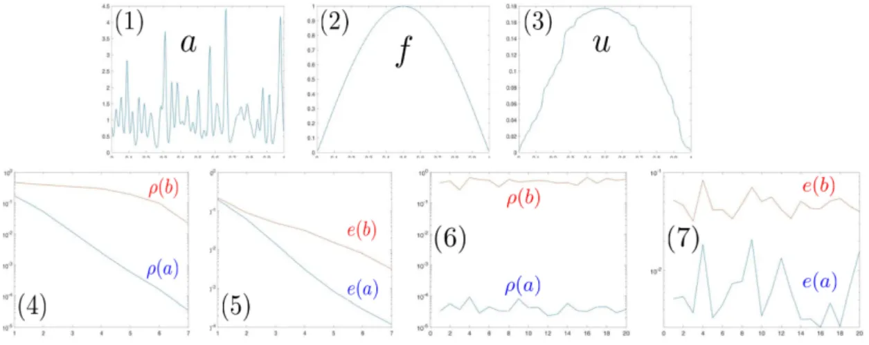
Figure 5: (1) a (2) f (3) u (4) ρ(a) and ρ(b) vs k, geometric (5) e(a) and e(b) vs k, geometric (6) ρ(a) and ρ(b) vsk, random (5) e(a) and e(b) vs random realization.
Which kernel should be used for the recovery of u when the conductivity a is un-known? Consider the case when d= 1 and Ω is the interval (0,1). Forb∈ L∞(Ω) with essinfΩ(b) > 0 write Gb for the Green’s function of the operator −div(b∇·) mapping
H1
0(Ω) toH−1(Ω). Observe that the {Gb|b} is a set of kernels parameterizedb and any kernel in that set could be used to interpolate the data. Which one should we pick? The answer proposed in Sec. 3and4 is to use the ordering induced byρto select the kernel.
Fig. 5 provides a numerical illustration of that ordering. In that example Ω is dis-cretized over 28 equally spaced interior points (and piecewise linear tent finite elements) and Fig. 5.1-3 shows a, f and u. For k ∈ {1, . . . ,8} and i ∈ I(k) := {1, . . . ,2k−1} let x(ik)=i/2k and write vb(k) for the interpolation of the data (xi(k), u(x(ik)))i∈I(k) using
the kernel Gb (note that vb(8) =u). Let kvkb be the energy normkvk2b =
R Ω(∇v)
Tb∇v. Take b ≡ 1. Fig. 5.4 shows (in semilog scale) the values of ρ(a) = kv
(k) a −v(8)a k2a kv(8)a k2a and ρ(b) = kv (k) b −v (8) b k2b kvb(8)k2 b
vs k. Note that the value of ratio ρ is much smaller when the kernel
Ga is used for the interpolation of the data. The geometric decayρ(a)≤C2−2k
kfkL2(Ω) kuk2
a is well known and has been extensively studied in Numerical Homogenization [21].
Fig. 5.5 shows (in semilog scale) the values of the average prediction errorse(a) and
kvb(k)(x)−u(x)kL2(Ω). Note again that the prediction error is much smaller when the
kernelGa is used for the interpolation.
Now let us consider the case where the interpolation points form a random subset of the discretization points. Take Nf = 27 and Nc = 26. Let X = {x1, . . . , xNf} be a subset Nf distinct points of (the discretization points) {i/28|i ∈ I(8)} sampled with uniform distribution. Let Z = {z1, . . . , zNc} be a subset of Nc distinct points of X sampled with uniform distribution. Writevbf for the interpolation of the data (xi, u(xi)) using the kernel Gb and write vbc for the interpolation of the data (zi, u(zi)) using the kernel Gb. Fig. 5.6 shows in (semilog scale) 20 independent random realizations of the values of ρ(a) = kvfa −vack2a/kv f ak2a and ρ(b) = kv f b −vbck2b/kv f bk2b. Fig. 5.7 shows in (semilog scale) 20 independent random realizations of the values of the prediction errors
e(a)∝ ku−vackL2(Ω) and e(b) ∝ ku−vbckL2(Ω). Note again that the values of ρ(a), e(a)
are consistently and significantly lower than those of ρ(b), e(b).
Figure 6: (1)aand b forn= 1 (2)a andb forn= 350 (2) ρ(b) vsn(4) e(b) vsn.
Fig. 6 provides a numerical illustration of an implementation of Alg. 1 with Nf =
N = 27,Nc= 26 andnc= 1. In this implementationa, f anduare as in Fig.5.1-3. The training data corresponds toNf points X={x1, . . . , xNf} uniformly sampled (without replacement) from {i/28|i∈ I(8)} (SinceN = N
f these points remain fixed during the execution the of the algorithm). n. The purpose of the algorithm is to learn the kernel
Ga in the set of kernels{Gb(W)|W} parameterized by the vectorW via
logb(W) = 26
X
i=1
(Wiccos(2πix) +Wissin(2πix)). (5.2)
Usingn to label its progression, Alg.1 is initialized at n= 1 with the guess b≡1 (i.e.
W ≡ 0) (Fig. 6.1). At each step (n → n+ 1) the algorithm performs the following operations:
1. SelectNcpointsZ ={z1, . . . , zNc}uniformly sampled (without replacement) from
2. Writevbf andvfc for the interpolation of the data (xi, u(xi)) and (zi, u(zi)) using the kernelGb, andρ(W) =kvbf −vcbk2b/kv
f
bk2b. Compute the gradient ∇Wρ(W) using Cor.4.1(and the identity∂WiΘ(W) =−π0(A0(W))
−1∂ WiA0(W)(A0(W)) −1πT 0 for Θ(W) =π0(A0(W))−1π0T). 3. UpdateW →W −λ∇Wρ(W) (with λ∝0.01/k∇Wρ(W)kL2).
Fig.6.2 shows the value of bforn= 350. Fig.6.3 shows the value ofρ(b) vsn. Fig.6.4 shows the value of the prediction errore(b)∝ ku−vbckL2(Ω) vsn. The lack of smoothness
of the plots of ρ(b), e(b) vsnoriginate from the re-sampling of the setZ at each stepn.
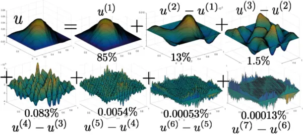
Figure 7: u and u(k)−u(k−1). Number below sub-figures show relative energy content
ku(k)−u(k−1)k2/kuk2. Used from forthcoming book [21] with permission from Cambridge University Press.
Remark 5.1. For d ≥ 1, let Ω = (0,1)d and for k ≥ 1, let τi(k) be a nested (in
k) hierarchy of sub-cubes of (0,1)d with locations indexed by i. For L = −div(a∇)
let ξ ∼ N(0,L−1) and let u(k) := E[ξ | Rτ(x)
i
ξ = Rτ(x)
i
ξu for all i]. Fig. 7 shows (for d = 2) the corresponding increments u(k) −u(k−1) and the relative energy con-tent ku(k)−u(k−1)k2/kuk2 of each increment for a solution of (5.1) with f ∈ L2(Ω). The quick decay of ku(k)−u(k−1)k2/kuk2 with respect to k illustrates the accuracy of the Green’s function of (5.1) used as a kernel for interpolating partial linear measure-ments made on solutions of (5.1). This numerical homogenization phenomenon [21,18] is one motivation for minimizing ρ in the kernel identification problem described above (ku(k)−u(k−1)k2/kuk2 ≈ρ
6
Kernel Flows (KF)
6.1 Non parametric family of kernels and bottomless networks without guesswork
Composing a symmetric positive kernel with a function produces a symmetric positive kernel [4]. We will now use this property to learn a kernel from the data within a non-parametric family of kernels constructed by composing layers of functions. For n ≥ 2 let Gn : X → X (X is the input space mentioned Pb. 1) be a sequence of functions determining the layers of this network. Let > 0 be a small parameter, let F1 := Id be the identity function and for n≥2, let Fn be the sequence of functions inductively defined by
Fn+1= (Id+Gn+1)◦Fn. (6.1) Let Kn be the sequence of symmetric positive kernels obtained by composing a kernel
K1 with this sequence of functions, i.e. Kn(x, x0) =K1(Fn(x), Fn(x0)) and
Kn+1(x, x0) =Kn x+Gn+1(x), x0+Gn+1(x0)
. (6.2)
Our purpose is to use the training data (x1, y1), . . . ,(xN, yN) ∈ X × Y to learn the functions G1, . . . , Gn∗ and then approximate u† with un∗ obtained by interpolating a
subset of the training data withKn∗.
When applied to a classification problem with n = 1 the proposed algorithm is a support-vector network (in the sense of [3]) with kernelK1. Asnprogresses the algorithm incrementally modifies the kernel via small perturbations of the identity operator (Gn+1 is reminiscent of the residual term of deep residual networks [8]). Since the training does not require any back propagation, achieving profound depths (with 10000 layers or more) is not difficult (since training is akin to simulating a stochastic dynamical system the network is essentially bottomless) and one purpose of this section is to explore properties of such bottomless networks (see [9] for a review of the motivations/challenges associated with the exploration of very deep networks).
6.2 The algorithm
We will adapt Algorithm 1 to learn the functions G1, . . . , Gn, . . . by induction over n. As in Sec. 4let Nf ≤N andNc= round(Nf/2).
For n= 1 let x(in):=xi fori∈ {1, . . . , N}.
Letn≥1. Assumex(1n), . . . , xN(n)to be known. Letsf,n(1), . . . , sf,n(Nf) beNf distinct elements of {1, . . . , N} obtained through random sampling (with uniform distribution) without replacement. Letsc,n(1), . . . , sc,n(Nc) beNcdistinct elements of{1, . . . , Nf}also obtained through random sampling (with uniform distribution) without replacement. Letπ be the correspondingNc×Nf sub-sampling matrix defined byπi,j(n)=δsc,n(i),j. Let
yf(n)∈RNf andy(n)
c ∈RNc be the corresponding subvectors ofydefined byyf,i(n)=ysf,n(i) andyc,i(n)=yf,sc,n(i). Fori∈ {1, . . . , Nf}letx(f,in) :=x(sn)
f,n(i)and write Θ
(n)for theN f×Nf matrix with entries
Θi,j(n)=K1(xf,i(n), x(f,jn)), (6.3) and let ρ(n) := 1−(y (n) c )T(π(n)Θ(n)(π(n))T)−1y(cn) (yf(n))T(Θ(n))−1y(n) f . (6.4)
Let ˆyf(n):= (Θ(n))−1yf(n), ˆz(fn):= (π(n))T(π(n)Θ(n)(π(n))T)−1π(n)yf(n)and fori∈ {1, . . . , Nf} let ˆ g(f,in):= 2(1−ρ(n))ˆy (n) f,i(∇xK1)(x (n) f,i, x (n) f,·)ˆy (n) f −ˆz (n) f,i(∇xK1)(x (n) f,i, x (n) f,·)ˆz (n) f yTf(Θ(n))−1y f (6.5)
LetGn+1 be the function obtained by interpolating the data (xf,i(n),ˆg(f,in)) with the kernel
K1, i.e. Gn+1(x) = (ˆg(f,n·))T K1(x(f,n·), x (n) f,·) −1 K1(x(f,n·), x). (6.6) Note thatG(n+1)(x(f,in)) = ˆgf,i(n). For i∈ {1, . . . , N}, let
x(in+1)=x(in)+Gn+1(x(in)). (6.7)
Remark 6.1. In the description above the input spaceX (of the functionu to be inter-polated) is assumed to a finite-dimensional vector space and the output space Y (of the functionuto be interpolated) is assumed to be contained in the real lineR. If the output
space Y is a finite-dimensional vector space (e.g. RdY) then y(fn) and yc(n) are Nf ×dY and Nc×dY matrices and (6.4) and (6.5) must be replaced by
ρ(n) := 1−Tr (y(cn))T(π(n)Θ(n)(π(n))T)−1y(cn) Tr (yf(n))T(Θ(n))−1y(n) f . (6.8) and ˆ g(f,in):= 2Tr (1−ρ(n))ˆyf,i(n)(∇xK1)(x(f,in), x(f,n·))ˆy (n) f −zˆ (n) f,i(∇xK1)(x (n) f,i, x (n) f,·)ˆz (n) f TryTf(Θ(n))−1y f , (6.9) where, in (6.9), yˆf,i(n) ∈ RdY, yˆ(n) f ∈ RNf ×dY, (∇ xK1)(x (n) f,i, x (n) f,·) ∈ RdX ×Nf (writing d X for the dimension of the input space,∇xK1 refers to the gradient over the first component of K1). The product results in a dY ×dX ×dY tensor and the trace (taken with respect to the dY dimensions) results in a vector in RdX, i.e. writing xs for the sth entry of x, (ˆgf,i(n))s = 2 PdY l=1 PNf t=1(1−ρ(n))(ˆy (n) f )i,l∂xsK1(x(f,in),x (n) f,t)(ˆy (n) f )t,l−(ˆz (n) f )i,l∂xsK1(x(f,in),x (n) f,t)(ˆz (n) f )t,l TryT f(Θ(n))−1yf .
This simple modification (via the trace operator) is equivalent to endowing the space of functions v= (v1, . . . , vdY) mapping X to Y with the RKHS norm kvk
2 =PdY i=1kvik2 with kvik2 = supφ (R Xφ(x)vi(x)dx)2 R
X2φ(x)Kn(x,x0)φ(x0)dx dx0 and using that norm to compute ρ and its
gradient.
6.3 Rationale of the algorithm
Observe that the algorithm is randomized through the random samplessf,n(i) andsc,n(i) (taking values in the training data). Observe also that, given those random samples, the functions Gn, Fn and kernels Kn are entirely determined by the values of the learning parameters ˆgf,i(n)=G(n+1)(x(f,in)).
As in Alg. 1, the ˆgf,i(n) are selected in (6.5) in the direction of the gradient descent of the ratio ρ: we apply Prop. 3.2 to compute the Frech´et derivative of ρ(n) (6.4) with respect to small perturbationsx(f,in)+g(f,in)to thex(f,in) and select thegf,i(n)in the direction of the gradient descent.
More precisely letgf,i(n)be candidates for the values ofG(n+1)(x(f,in)) and write ˜x(f,in+1)=
xf,i(n)+gf,i(n). Write ˜Θ(n+1) for theN
f ×Nf matrix with entries ˜ Θi,j(n+1) =K1(˜xf,i(n+1),x˜(f,jn+1)), (6.10) and let ˜ ρ(n+ 1) := 1−(y (n) c )T(π(n)Θ˜(n+1)(π(n))T)−1yc(n) (yf(n))T( ˜Θ(n+1))−1y(n) f . (6.11)
Then the following proposition identifies ˆgf,i(n) as the direction of the gradient descent of ˜
ρ(n+ 1) with respect to the parameters g(f,in).
Proposition 6.2. It holds true that
˜ ρ(n+ 1) =ρ(n)− Nf X i=1 (gf,i(n))Tˆgf,i(n)+O(2). (6.12)
where thegˆf,i(n) are as in (6.5).
Proof. We deduce from (6.2) that, to the first order in ,
Kn+1(x, x0)≈Kn x, x0
+ (Gn+1◦Fn(x))T(∇xK1) Fn(x), Fn(x0) + (Gn+1◦Fn(x0))T(∇x0K1) Fn(x), Fn(x0).
(6.13)
Therefore, using the symmetry of K1, we have ˜
with
Ti,j(n)= (gf,i(n))T(∇xK1)(x(f,in), xf,j(n)) + (gf,j(n))T(∇xK1) x(f,jn), x(f,in)). (6.15) We deduce from Proposition3.2 that
ρ( ˜Θ(n+1)) =ρ(Θ(n))−(1−ρ(Θ (n)))(ˆy(n) f )TT(n)yˆ (n) f −(ˆz (n) f )TT(n)zˆ (n) f (ˆyf(n))TΘ(n)yˆ(n) f +O(2), (6.16)
which implies the result after simplification.
The following corollary is a direct application of Prop.6.2.
Corollary 6.3. Let K1(x, x0) =e−γ|x−x
0|2
. It holds true that
ρ( ˜Θ(n+1)) =ρ(Θ(n))− Nf X i=1 (g(in))Tˆgi(n)+O(2). (6.17) withgˆi(n):= 4γ (y(fn))T(Θ(n))−1y(n) f PNf j=1Γ (n) i,j x (n) f,j,
Γ(i,jn) =δi,jzˆ(f,in)(Θ(n)zˆ(n))f,i−zˆf,i(n)Θ(i,jn)zˆ (n) f,j
−(1−ρ(Θ(n)))δi,jyˆf,i(n)yf,i(n)+ (1−ρ(Θ(n)))ˆyf,i(n)Θ(i,jn)yˆf,j(n).
(6.18)
and zˆf(n)= (π(n))T(π(n)Θ(n)(π(n))T)−1π(n)yf, yˆf(n)= (Θ(n))−1y(fn).
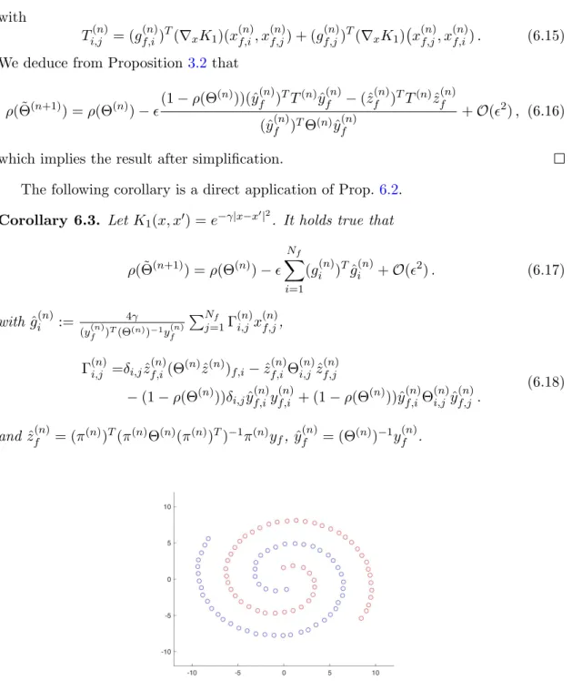
Figure 8: Swiss Roll Cheesecake. N = 100. Red points have label −1 and blue points have label 1.
7
The Flow of the KF algorithm on the Swiss Roll
cheese-cake
From a numerical analysis perspective, the flow Fn(x) associated with the Sec. 6 KF algorithm approximates, in the sense of Smoothed Particle Hydrodynamics [7], a flow
F(t, x) mapping R× X into X. Writing xi for the N training data points in X, as
↓ 0, Fn(xi) approximates Xi(t) := F(t, xi) which (after averaging the effect of the randomized batches) can be identified as the solution of a system of ODEs of the form
dX
dt =G(X, N, Nf, K1). (7.1)
7.1 Implementation of the KF algorithm
We will now explore a few properties of this approximation by implementing the KF algorithm for the Swiss Roll Cheesecake illustrated in Fig. 8. The dataset is composed ofN = 100 pointsxi inR2 in the shape of two concentric spirals. Red points have label
−1 and blue points have label 1. Since our purpose is limited to illustrating properties of the discrete flow Fn(x) associated with the Kernel Flow algorithm we will consider all those points as training points (will not introduce a test dataset) and visualise the trajectoriesn→Fn(xi) of the data pointsxi.
The KF algorithm is implemented with the Gaussian kernel of Corollary 6.3 with
γ−1 = 4. Training is done in random batches of size Nf and we use Nc = Nf/2 to compute the ratio ρ and learn the parameters of the network. We start with Nf =N and as training progresses points of the same color start merging. Therefore to avoid near singular matrices caused by batches with points of the same color sharing nearly identical coordinates, once the distance between two points of the same color is smaller than 10−4 (in Fig.3,9and10) we drop one of them out of the set of possible candidates for the batch and decrease Nf by 1 (the point left out remains advected byGn+1 but is simply no longer available as an interpolation point defining Gn+1).
Fig. 3showsFn(xi) vsnfor 1≤n≤7000. In Fig.3the value of is chosen at each step n so that the perturbation of each data point xi of the batch is no greater than
p% with p = 10 for 1≤n≤1000 and p = 10/pn/1000 for n≥1000. The two spirals quickly unroll into two linearly separable clusters.
Fig. 9 showsFn(xi) vs n for 1≤n≤500000. The value of is chosen at each step
n so that the perturbation of each data point xi of the batch is no greater than 0.5%. The two intertwined spirals unroll into straight (vibrating) segments. The final unrolled configuration appears to be unstable (some red points are ejected out of the unrolled red segment towards the end of the simulation) and although this instability seems to be alleviated by adjusting to a smaller value at the end of the simulation it seems to also be caused by a combination of (1) the stiffness of the flow being simulated (2) the process of permanently removing points from the pool of possible candidates for the batch. Although these points remain advected by the flow and are initially at distance
Figure 9: Fn(xi) for 8 different values of n. is chosen at each step n so that the perturbation of each data pointxi of the batch is no greater than 0.5%.
less than 10−4 of a point of the same color, the stiffness of the flow can quickly increase this distance and separate the point from its group ifis not small enough.
7.2 Addition of nuggets
The instabilities observed in Fig.9 seem to vanish (even with significantly larger values of) after the addition of a nugget (white noise kernel accounting for measurement noise in kriging) to the kernel K1. In Fig. 10 we consider a longer version of the Swiss Roll Cheesecake (N = 250). The kernel isK1(x, x0) =e−γ|x−x
0|2
+δ(x−x0)e−γ62 (γ−1= 4).
is chosen at each step n so that the absolute perturbation (maximum translation) of each data point xi of the batch is no greater than 0.05. Fig. 10 shows Fn(xi) vsn for 1 ≤n≤500000. The two intertwined spirals unroll into stable clusters slowly drifting away from each other.
7.3 Instantaneous and average vector fields
With the addition of the nugget, the permanent removal of close points from the pool of candidates is no longer required for avoiding singular matrices. In Fig.11,12 and 13
(see [25] for videos) we consider the N = 100 version of the Swiss Roll Cheesecake. The kernel isK1(x, x0) =e−γ|x−x
0|2
+δ(x−x0)e−γ62 (γ−1 = 4). is chosen at each stepnso that the absolute perturbation (maximum translation) of each data pointxi of the batch is no greater than 0.2. Only a nugget is added and close points are not removed from the pool of candidates (which eliminates the instabilities observed in Fig. 9). Fig. 11
Figure 10: N = 250. Fn(xi) for 8 different values of n. is chosen at each step n so that the absolute perturbation of each data pointxiof the batch is no greater than 0.05.
K1(x, x0) =e−γ|x−x0|2+δ(x−x0)e−γ62
Figure 11: Fn(xi) and decision boundary for 8 different values of n.
shows Fn(xi) vs n for 1 ≤ n ≤ 180000 and the decision boundary between the two classes vs n. The two intertwined spirals unroll into stable clusters. Fig. 12 shows the instantaneous velocity field Fn+1(x)−Fn(x). Fig. 13 shows the average velocity field 10(Fn+300(x)−Fn(x))/300. The difference between the instantaneous and average velocity fields is and indication of the presence of multiple time scales caused by the
Figure 12: Instantaneous velocity fieldFn+1(x)−Fn(x). (1-4) show 4 successive values. (5) shows the instantaneous velocity field for the final configuration.
randomization process and the stiffness of the underlying flow. 7.4 The continuous flow.
The intriguing behavior of these flows, calls for their investigation from the a numerical integration perspective (note that an ODE perspective emerges as ↓ 0, an SDE per-spective is relevant whenis non-null due to the randomization of the batches, a PDE perspective emerges as ↓ 0 andN → ∞, and an SPDE approximation perspective is relevant when is non-null andN is finite).
Note that the KF flow Fn(x) can be seen (as↓0) as the numerical approximation of a continuous flowF(t, x). identified as the solution of the dynamical system
∂F(t, x) ∂t =−EX,π " ∇Zρ(X, Z, π) T K1(Z, Z)−1K1 Z, x Z=F(X,t) # , (7.2)
with initial conditionF(0, x) =xand where the elements of (7.2) are defined as follows.
X is a random vector of XNf representing the random sampling of the training data in a batch sizeNf. Writing u(X)∈ YNf for the vector whose entries are the labels of the entries ofX ∈ XNf and π for a random N
c×Nf matrix corresponding to the selection of Nc elements at out Nf (at random, uniformly, without replacement), ρ, in (7.2), is defined as follows
ρ(X, Z, π) = 1−u(X)
TπT(K1(πZ, πZ))−1πu(X)
u(X)T(K1(Z, Z))−1u(X) . (7.3) The average vector field in Fig. 13 is an approximation of the right hand side of (7.2)
Figure 13: Average velocity field 10(Fn+300(x)−Fn(x))/300 for 5 different values of n.
and the convergence of Fround(t/)(x) towards F(t, x) as ↓ 0 is in the sense of two-scale flow convergence described in [33].
NI Average error Min error Max error Standard Deviation 6000 0.014 0.0136 0.0143 1.44×10⁻⁴
600 0.014 0.0137 0.0142 9.79×10⁻⁵ 60 0.0141 0.0136 0.0146 2.03×10⁻⁴ 10 0.015 0.0136 0.0177 7.13×10⁻⁴
Table 1: MNIST test errors using NI interpolation points
8
Numerical experiments with the MNIST dataset
We will now implement, test and analyze the Sec.6KF algorithm on the MNIST dataset [37]. This training set is composed of 60000, 28×28 images of handwritten digits (partitioned into 10 classes) with a corresponding vector of 60000 labels (with values in
{1, . . . ,9,0}). The test set is composed of 10000, 28×28 images of handwritten digits with a corresponding vector of 10000 labels.
Figure 14: Results for MNIST. N = 60000, Nf = 600 and Nc = 300. (1) Test error vs depthnwithNI= 6000 (2) Test error vs depthnwithNI = 600 (3) Test error vs depth
n with NI = 60 (4) Test error vs depth n with NI = 10 (5,6) Test error vs depth n withNI= 6000,600,60,10 (7)ρvs depthn(8) Mean-squared distances between images
Fn(xi) (all, inter class and in class) vs depth n (9) Mean-squared distances between images (all) vs depth n (10) Mean-squared distances between images (inter class) vs depth n (11) Mean-squared distances between images (in class) vs depth n (12) Ratio (10)/(11).
8.1 Learning with small random batches of the full training dataset. We first implement the Sec. 6 KF algorithm with the full training set, i.e. N = 60000. Images are normalized to haveL2 norm one and we use the Gaussian kernel of Corollary
6.3 and set γ−1 equal to the mean squared distance between training images. Training is performed in random batches of size Nf = 600 and we use Nc= 300 to compute the ratioρ and learn the parameters of the network (we do not use a nugget and we do not exclude points that are too close from those batches). The value of is chosen at each stepnso that the perturbation of each data pointxi of the batch is no greater than 1% (= 0.01×maxi
|x(f,in)|L2
|ˆg(f,in)|L2
).
Classification of the test data is performed by interpolating a subset of NI im-ages/labels (xi, yi) of the training data with the kernel Kn (the kernel at step/layer
Figure 15: Results for MNIST. N = 60000,Nf = 600 and Nc = 300. (1, 3, 5) Training data xi (2, 4, 6) Fn(xi) for n= 12000 (7)Fn(xi)−xi for training data and n= 12000 (8) Test data xi (9) Fn(xi) for test data and n= 12000 (10) Fn(xi)−xi for test data and n= 12000.
is a unit vector ej in R10 pointing in the direction of the class of the images (e.g. yi = (1,0,0,0,0,0,0,0,0,0) =e1if the class of imagexiisj= 1 andyi= (0,0,0,0,0,0,0,0,0,1) =
e10 if the class of image xi is j = 0). The interpolant un is a function from R28×28 to R10 and the class of an imagex is simply identified as argmaxjeTj ·un(x). The Sec. 6.2 Kernel Flow algorithm is implemented (using Remark 6.1) with N = 60000, Nf = 600 and Nc= 300 and ended forn= 12000 (resulting in a network with 12000 layers).
Table1shows test errors (with the test data composed of 10000 images) obtained with
NI = 6000,600,60 and 10 interpolation points (selected at random uniformly without replacement and conditioned on containing an equal number of example from each class to avoid degeneracy for NI = 10,60). The second column shows errors averaged over the last 100 layers of the network (i.e. obtained by interpolating the NI data points with Kn for n = 11901,11902, . . . ,12000). The third, fourth and fifth columns show the min, max and standard deviation of the error over the same last 100 layers of the network. Surprisingly, around layer n= 12000, the kernel Kn achieves an average error of about 1.5% with only 10 data points (by using only 1 random example of each digit as an interpolation point). Multiple runs of the algorithm suggest that those results are
stable.
Fig.14shows test errors vs depthn(withNI = 6000,600,60,10 interpolation points), the value of the ratio ρ vs n (computed with Nf = 600 and Nc = 300) and the mean squared distances between (all, inter class and in class) images Fn(xi) vs n. Observe that all mean-squared distances increase until n ≈ 7000. After n ≈ 7000 the in class mean-squared distances decreases withnwhereas the inter-class mean-squared distances continue increasing. This suggests that aftern≈7000 the algorithm starts clustering the data per class. Note also that while the test errors, with NI = 6000,600 interpolation points, decrease immediately and sharply, the test errors with NI = 10 interpolation points increase slightly untiln≈3000 towards 60%, after which they drop and seem to stabilize around 1.5% towardsn≈10000.
It is known that iterated random functions typically converge because they are con-tractive on average [5, 6]. Here training appears to create iterated functions that are contractive with each class but expansive between classes.
Fig.15 shows 10×xi and 10×Fn(xi) and 20×(Fn(xi)−xi) forn= 12000, training images and test images. The algorithm appears to introduce small, archetypical, and class dependent, perturbations in those images.
Figure 16: (1) Test error vsn(2)ρvsn(3)xi andFn(xi) forn= 8000 andi correspond-ing to the first 12 traincorrespond-ing images (4)xi andFn(xi) forn= 8000 andicorresponding to the first 12 test images. MNIST with classes 2 and 4, 600 training images and 100 test images.
8.2 Bootstrapping, Brittleness and Data Archetypes
In Sec.8.1we used the whole training set ofN = 60000 images to train our network and Fig. 14. Although the accuracy the network increases (between n = 1 andn = 12000) when using onlyNI= 6000,600,60,10 interpolation points, the accuracy of the network with NI = 60000 (the full training set as interpolation points) does not seem to be significantly impacted by the training (the error withNI = 60000 is 0.0128 atn= 1 and
Figure 17: MNIST with all classes, 1200 training images and 2000 test images. (1) Test error vs n(2)ρ vs n(3) Training imagesxi (4) 10×abs(Fn(xi)−xi) for n= 900
the information contained in the 60000 data-points to the kernelKn. Can the accuracy of the interpolation with the full training set be improved? Can the algorithm extract information that cannot already be extracted by performing a simple interpolation (with a simple Gaussian kernel) with the full training dataset? To answer these questions we will now implement the Sec.6.2Kernel Flow algorithm with subsets of training and test images and train the network with Nf =N (the size of each batch is equal to the total number of training images), Nc = Nf/2 and possibly subsets of the set of all classes. We work with raw images (not normalized to have L2 norm one). We use the Gaussian kernel of Corollary6.3 and identifyγ−1 as the mean squared distance between training images. We first take N = 600 (600 training images) showing only twos and fours and attempt to classify 100 test images (with only twos and fours). Fig.16 corresponds to a successful outcome (with small adapted step sizes ) and shows the test error vs depth
n,ρ vs nand xi and Fn(xi) forn= 8000. These illustrations suggest that the network can bootstrap data and improve accuracy by introducing small (nearly imperceptible to the naked eye) perturbations to the dataset. Fig.17 shows another successful run with
N = 1200 training images, 1200 test images and the full set of 10 classes.
Mode collapse from going too deep, too fast, with Nf = N. Fig. 18 shows a failed outcome (with very large step sizes , the other parameters are the same as in Fig.16). Although the ratioρ decreases during training the error blows up towards 50% and theFn(xi) seem to collapse towards two images: a four and a random blur. We will explain and analyze this mode collapse below.
8.3 Mode collapse, brittleness of deep learning
The mode collapse observed in Fig. 18 is interesting for several reasons. First it shows that a decreasingρis not sufficient to ensure generalization and learning. Indeed writing
w for a function exactly interpolating (fitting) the training data the kernel Kw(x, y) =
w(x)w(y) would lead to a perfect fit (and hence a value ρ= 0) of the training set with any number of interpolation points (and in particular one). Although thisKwis positive but degenerate, if the space of kernels explored by the algorithm is large enough, then,
Figure 18: MNIST with classes 2 and 4, 600 training images and 100 test images. Step sizes are too large, ρ decreases but the modes collapse. (1) xi and Fn(xi) for
n= 1,100,1800 andicorresponding to the first 12 training images (2)xi andFn(xi) for
n= 1,100,1800 and icorresponding to the first 12 test images (3) ρ vsn(4) Test error vsn
unless Nf N, it is not clear what would prevent the algorithm from over-fitting and converging towards those pathological kernels.
The brittleness of deep learning [32] is a well known phenomenon predicted [15] from the brittleness of doing inference in large dimensional spaces [22,19,23, 26]. The mechanisms at play in [23] suggest that those instabilities may be unavoidable if the inference space is too large and could to some degree be alleviated through a compromise between accuracy and robustness [26]. From that perspective the learning of the Green’s function in Sec.5appears to be stable because of strong constraints imposed on the space of kernels (by the structure of the underlying PDE). In Sec. 8.1 the difference in size between the training dataset (N) and that of the batches (Nf) seems to have a stabilizing effect on the algorithm. The pathologies observed in Fig. 18, and mechanisms leading to brittleness [22, 19, 23, 26, 17] seem to suggest that will small data sets and a large space of admissible kernels instabilities may occur and could be alleviated by introducing further constraints on the space of kernels.
8.4 Classification archetypes
The brittleness of deep learning [22, 32] has lead to the construction of libraries of adversarial examples whose persistence in the physical work [12] be exploited by an adversary [10]. These adversarial examples are constructed via small (near-undetectable to the naked eye) data-dependent (non-random) perturbations of the original images. The Kernel Flow algorithm seems to exploit the brittleness of deep learning in the opposite direction (towards improved performance), i.e. as suggested in Fig.15 and 16
the Kernel Flow algorithm seems to improve performance through the construction of residual maps introducing small (data-dependent) perturbations to the original images. The resulting images Fn(xi) at profound depths could be interpreted as archetypes of the classes being learned.
Figure 19: Minimizing mean squared interpolation error rather than ρ may not lead to generalization for KF. (1) Mean squared interpolation errore2(n) calculated with random subsets of the training data (Nf = 600 and Nc= 300) (2) Mean squared interpolation errore2(n) calculated with the test data (NI= 6000) (3) Classification accuracy (using
NI = 6000 interpolation points and all 10000 test data points) vs n (4) Classification accuracy (using NI = 600 interpolation points and all 10000 test data points) vs n.
8.5 On generalization
Why the KF algorithm does not seem to overfit the data? Why is it capable of general-ization? From an initial perspective the KF algorithm appears to promote generalization by grouping data points into clusters according to their classes. However the reason for its generalization properties appears to be more subtle and definingρthrough the RKHS norm seems to also play a role (minimizingρby aligning the eigensubpace corresponding to the lowest eigenvalues of the kernel with the training data.).
Indeed, using the notations of Sec. 6, let v(x(f,in)) be the predicted labels of the Nf points x(f,in) obtained by interpolating a random subset of Nc = Nf/2 points (xi, yi) with the kernel K1 and write e2 := P
Nf i=1|y
(n) f,i −v(x
(n)
f,i)|2 for the mean squared error between training labels and predicted labels. Then minimizinge2 instead of ρ may lead to a decreasing test classification accuracy rather than an increasing one as shown in Fig. 19 (using the MNIST dataset with N = 60000 training points, 10000 test points,
Nf = 600,Nc= 300 for the random batches andNI= 600,6000 interpolation points for calculating classification accuracies). Note that although the mean squared interpolation error decreases for the training and the test data, the classification error (on the 10000 test data points of MNIST using 6000 interpolation points) increases.
NI Average error Min error Max error Standard Deviation 6000 0.0969 0.0944 0.1 7.56×10⁻⁴
600 0.0977 0.0951 0.101 8.57×10⁻⁴ 60 0.114 0.0958 0.22 0.0169 10 0.444 0.15 0.722 0.096
Table 2: Fashion-MNIST test errors (between layers 15000 and 25000) using NI inter-polation points
NI Average error Min error Max error Standard Deviation 6000 0.10023 0.0999 0.1006 1.6316×10⁻⁴ 600 0.10013 0.0999 0.1004 1.1671×10⁻⁴ 60 0.10018 0.0999 0.1005 1.445×10⁻⁴ 10 0.10018 0.0996 0.1009 2.2941×10⁻⁴
Table 3: Fashion-MNIST test errors (between layers 49901 and 50000) using NI inter-polation points
9
Numerical experiments with the Fashion-MNIST dataset
We now implement and test the Sec. 6KF algorithm with the Fashion-MNIST dataset [36]. As with the MNIST dataset [37], the Fashion-MNIST dataset is composed of 60000, 28×28 images portioned into 10 classes (T-shirt/top, trouser, pullover, dress, coat, sandal, shirt, sneaker, bag, ankle boot) with a corresponding vector of 60000 labels (with values in{0, . . . ,9}). The test set is composed of 10000, 28×28 images of handwritten digits with a corresponding vector of 10000 labels.
9.1 Network trained to depth n= 50000
The KF algorithm is implemented with the exact same parameters as for the MNIST dataset (Sec.8.1, in particular it does not require any manual tuning of hyperparameters nor a laborious process of guessing an architecture for the network). In particular, images are normalized to haveL2 norm one we use the Gaussian kernel of Corollary6.3and set
γ−1 equal to the mean squared distance between training images. Training is performed in random batches of size Nf = 600 and we use Nc = 300 to compute the ratio ρ and learn the parameters of the network (we do not use a nugget and we do not exclude points that are too close from those batches). The value of is chosen at each step
n so that the perturbation of each data point xi of the batch is no greater than 1% (= 0.01×maxi
|x(f,in)|L2
|ˆg(f,in)|L2
).
The network is trained to depthn= 50000. Table2shows test error statistics (on the full test dataset) using the kernelKn for 15000≤n≤25000 and NI = 6000,600,60,10
Figure 20: Results for Fashion-MNIST. N = 60000, Nf = 600 and Nc = 300. (1) Test error vs depthnwithNI = 6000 (2) Test error vs depthnwithNI= 600 (3) Test error vs depthnwithNI = 60 (4) Test error vs depthnwithNI= 10 (5,6) Test error vs depthn withNI= 6000,600,60,10 (7)ρvs depthn(8) Mean-squared distances between images
Fn(xi) (all, inter class and in class) vs depth n (9) Mean-squared distances between images (all) vs depth n (10) Mean-squared distances between images (inter class) vs depth n (11) Mean-squared distances between images (in class) vs depth n (12) Ratio (10)/(11).
interpolation points. Table 3 shows test error statistics (on the full test dataset) using the kernel Kn for 49901 ≤ n ≤ 50000 and NI = 6000,600,60,10 interpolation points. Fig.20plots test errors vsnusingNI = 6000,600,60,10 interpolation points and shows average distances betweenFn(xi) vsn(for xi selected uniformly at random amongst all training images, within the same or in different classes).
Note that although the network achieves an average test error of 9.7% between layers 15000 and 25000 withNI = 600, average test errors forNI = 60,10 interpolation points require a depth of more than 37000 layers to achieve comparable accuracies. Note that the average error around layer 50000 withNI = 10 interpolation points is 10% and does not seem to significantly depend on NI. The average error (≈ 9.7%) of the classifier withNI = 600,6000 interpolation points between layers 15000 and 25000 and the slight increase of average test errors with NI = 600,6000 interpolation points between layers 25000 and 50000 (from≈9.7% to≈10%) seem to decrease with the value of. (6.1) could
Figure 21: Results for Fashion-MNIST. N = 60000, Nf = 600 and Nc = 300. (1) Training dataxi (2)Fn(xi) training data andn= 50000 (3) Test data xi (9)Fn(xi) for test data andn= 50000.
be interpreted an underlying stochastic differential equation with an explicit scheme with time stepsand the efficiency of the resulting classifier seems to improve as ↓0.
Note from Fig. 20.(8-12), 21 and 4 that Fn(xi) converges towards an archetype of the class of xi and that (after layer n ≈ 25000) the KF algorithm contracts distances within each class while continuing to expand distances between different classes.
Interpolation with K1 and allNI =N = 60000 training points used as interpolation points results in 12.75% test error and interpolation with Kn with n = 50000 and all
NI =N = 60000 training points used as interpolation points results in 10% test error. Therefore the KF algorithm appears to bootstrap information contained in the training data in the sense discussed in Sec.8.2.
Figure 22: Results for Fashion-MNIST. N = 60000, Nf = 600 and Nc = 300. Left: Training dataxi for class 5. Right: Fn(xi) training data and n= 11000.
9.2 Sign of unsupervised Learning?
Fig. 22 shoesxi and Fn(xi) for a group of images in the class 5 (sandal). The network is trained to depth n = 11000 and the value of is chosen at each step n so that the perturbation of each data point xi of the batch is no greater than 10% ( = 0.1× maxi
|x(f,in)|L2
|ˆg(f,in)|L2
). Note that this value of is 10 times larger than the one of Sec. 9.1. Surprisingly the flow Fn accurately clusters that class (sandal) into 2 sub-classes: (1) high heels (2) flat bottom. This is surprising because the training labels contain no information about such sub-classes: KF has created those clusters/sub-classes without supervision.
10
Kernel Flows and Convolutional Neural Network
10.1 MNIST
The proposed approach can also be applied to families of kernels parameterized by the weights of a Convolutional Neural Network (CNN) [13]. Such networks are known to achieve superior performance by, to some degree, encoding (i.e. providing prior infor-mation about) known invariants (e.g. to translations) and the hierarchical structure of data generating distribution into the architecture of the network.
We will first consider an application the MNIST dataset [37] with L2 normalized test and training images. The structure of the CNN is the one presented in [1] and its first layers are illustrated in Fig. 23. Given an input/image x, the last layer produces a vectorF(x)∈R300 used for SVN classification [3] with the Gaussian kernelK(x, x0) =
F(xi) (writingxi for the training images).
Figure 23: Convolutional filters used for MNIST classification [1].
The training of the filters (weights of the network) is done as described in sections 3
and4using random batches ofNf = 500 images (sampled uniformly without replacement out of N = 60000 training images) and sub-batches of Nc = 250 images (sampled uniformly without replacement out of the batch of Nf = 500 images). As in Sec. 3, write v† andvs for optimal recoveries using the kernelK, and respectively, the batch of
Nf and the sub-batch ofNcinterpolation points.
Writing yi ∈ R10 for the label of the image xi, the relative approximation error (in the RKHS norm associated with K) caused by halving the number of points is (using, for simplicity, the notations of Sec.3 to describe the computation ofρ for one batch)
ρ= 1−Tr (y
TAy˜ )
Tr (yTAy). (10.1)
wherey∈RNf×10, ˜A, A∈RNf×Nf. We will also consider the mean squared error
e2 = 2 Nf Nf X i=1 yi−vs(xi) 2 , (10.2)
where the sum is taken over the Nf elements of the batch (note that yi −vs(xi) = 0 when iis in the sub-batch ofNc elements used as interpolation points for vs).
To train the network we simply let the Adam optimizer [11] in TensorFlow minimize
ρore2 (used as cost functions, which does not require the manual identification of their Fr´echet derivatives with respect to the weights of the network).
Table 4 shows statistics of the corresponding test errors using the kernelK learned above (using all N = 60000 images in batches of size Nf = 500) and five randomly se-lected subsets ofNI= 12000 training images as interpolation points. Each run consisted of 10000 iterations and test errors were calculated on the final iteration. Fig. 24 shows the values ofρ ande2 evaluated at every 100 iterations for both algorithms (minimizing
ρ and e2). When trained with relative entropy and dropout [30] Gorner reports [1] a minimum classification error of 0.65% testing every 100 iterations over 5 runs. Since we are using the same CNN architecture, this appears to suggest that the proposed ap-proach (of minimizing ρ ore2) might lead to better test accuracies than training with relative entropy and dropout.
Algorithm Average error Min error Max error Standard Deviation Minimizing e2 0.596% 0.55% 0.63% 0.032%
Minimizing ρ 0.640% 0.60% 0.70% 0.034%
Table 4: Test error statistics using NI = 12000 interpolation points at iteration 10000 over 5 runs.
Figure 24: (1) and (2) showρand e2 respectively evaluated at then-th batch using the
e2 minimizing network. (3) and (4) show analogous plots for theρ minimizing network.
10.1.1 Interpolation with small subsets of the training set
Fig.25shows test errors using the kernelK learned above (using allN = 60000 images in batches of sizeNf = 500) and randomly selected subsets ofNI = 30000,12000,6000,600,60,10 training images as interpolation points.
Tables 5 and 6 show test errors statistics using the kernel K (learned above with
Nf = 500) withNI = 6000,600,60,10 interpolation points sampled at random (all use the same convolutional filters obtained in a single optimization run). Averages, min, max and STD are computed over iterations between iterations 9900 to 10000 using 5 independent runs of the Adam optimizer [11] with ρand e2 as objective functions.
Observe that, although as with Kernel Flow, using only a small fraction of the training data as interpolation points is sufficient to achieve low classification errors (the minimum error with 10 interpolation points is 0.58%), interpolation with only one image
Figure 25: (1) Classification test errors forNI= 10,60,600,6000,12000,30000 evaluated at the n-th batch for 0≤n≤10000 using the network minimizinge2. (2) same as (1) with 1000≤n≤10000. (3), (4) same as (1), (2) for the network minimizing ρ.
NI Average error Min error Max error Standard Deviation 6000 0.575% 0.42% 0.72% 0.052%
600 0.628% 0.48% 0.83% 0.062% 60 0.728% 0.51% 1.23% 0.103% 10 1.05% 0.58% 4.81% 0.375%
Table 5: Test error statistics usingNI interpolation points between iterations 9900 and 10000 over 5 runs of optimizinge2.
NI Average error Min error Max error Standard Deviation 6000 0.646% 0.51% 0.78% 0.046%
600 0.676% 0.56% 0.82% 0.047% 60 0.850% 0.58% 3.98% 0.357% 10 4.434% 0.97% 18.91% 2.320%
Table 6: Test error statistics usingNI interpolation points between iterations 9900 and 10000 over 5 runs of optimizingρ.
Figure 26: A “bad” (top) and “good” (bottom) selection of 10 interpolation points.
per class appears to be more sensitive to the particular selection of 10 interpolation points. Fig.26shows an example of a “good” and a “bad” selection for the interpolation with 10 points.
of the last layer of the CNN with input x) is a possible explanation for this extreme generalization. Fig. 27 shows the average mean squared Euclidean distance between
F(xi) in the same class and in distinct classes. Note that the ratio between average square distances between two inter-class and two in-class points approaches 12 (for the network optimizinge2), suggesting that the map F clusters of images per class.
Figure 27: (1) Mean-squared distance between F(xi) (all, in-class, and inter-class) vs iterationnfor the network optimizinge2(2) Ratio between inter-class and in-class mean-squared distance for the network optimizinge2. (3) and (4) are identical except for the network which optimizes ρ.
10.2 Fashion MNIST
We now apply the proposed approach to the Fashion-MNIST database. The architecture of the CNN is derived from [2] and the first layers of the network are shown in Fig. 28.
Figure 28: Convolutional filters used for Fashion MNIST classification [2].
The classification of test images is done as in Sec. 10.1.
Table7shows test errors statistics (over 5 runs) after training (using 10000 iterations and computing test errors at the final iteration) by minimizingρore2(as defined in (10.1) and (10.2)) using NI = 12000 interpolation points Mahajan [2] reports a testing error of 8.6% when using the validation set to obtain the convolutional filters. As above, this suggests that the proposed approach could lead to better test accuracies than training
with relative entropy and dropout. Finally, Fig. 29 shows ρ and e2 evaluated at every 100 iterations for both algorithms.
Algorithm Average error Min error Max error Standard Deviation Optimizing e2 8.474% 8.24% 8.70% 0.147%
Optimizing ρ 8.412% 8.29% 8.56% 0.091%
Table 7: Test error statistics using NI = 12000 interpolation points at iteration 10000 over 5 runs.
Figure 29: (1) and (2) showρand e2 respectively evaluated at then-th batch using the
e2 minimizing network. (3) and (4) show analogous plots for theρ minimizing network.
10.2.1 Interpolation with small subsets of the training set
Fig.30shows test errors using the kernelK learned above (using allN = 60000 images in batches of sizeNf = 500) and randomly selected subsets ofNI = 30000,12000,6000,600,60,10 training images as interpolation points.
Further, the minimum errors in Fig. 30.1, 3 are observed to be 8.02% and 7.89% respectively, where both minima used NI = 30000.”