TI 2015-050/III
Tinbergen Institute Discussion Paper
Cyclicality in Losses on Bank Loans
Bart Keijsers
Bart Diris
Erik Kole
Erasmus School of Economics, Erasmus University Rotterdam, the Netherlands, and Tinbergen Institute, the Netherlands.
Tinbergen Institute is the graduate school and research institute in economics of Erasmus University Rotterdam, the University of Amsterdam and VU University Amsterdam.
More TI discussion papers can be downloaded at http://www.tinbergen.nl
Tinbergen Institute has two locations: Tinbergen Institute Amsterdam Gustav Mahlerplein 117 1082 MS Amsterdam The Netherlands Tel.: +31(0)20 525 1600 Tinbergen Institute Rotterdam Burg. Oudlaan 50
3062 PA Rotterdam The Netherlands Tel.: +31(0)10 408 8900 Fax: +31(0)10 408 9031
Duisenberg school of finance is a collaboration of the Dutch financial sector and universities, with the ambition to support innovative research and offer top quality academic education in core areas of finance.
DSF research papers can be downloaded at: http://www.dsf.nl/
Duisenberg school of finance Gustav Mahlerplein 117 1082 MS Amsterdam The Netherlands Tel.: +31(0)20 525 8579
Cyclicality in Losses on Bank Loans
∗Bart Keijsers† Bart Diris
Erik Kole
Econometric Institute, Erasmus School of Economics, Erasmus University Rotterdam Tinbergen Institute, Erasmus University Rotterdam
May 4, 2015
Abstract
Cyclicality in the losses of bank loans is important for bank risk management. Because loans have a different risk profile than bonds, evidence of cyclicality in bond losses need not apply to loans. Based on unique data we show that the default rate and loss given default of bank loans share a cyclical component, related to the business cycle. We infer this cycle by a new model that distinguishes loans with large and small losses, and links them to the default rate and macro variables. The loss distributions within the groups stay constant, but the fraction of loans with large losses increases during downturns. Our model implies substantial time-variation in banks’ capital reserves, and helps predicting the losses.
Keywords: Loss-given-default, default rates, credit risk, capital requirements, dynamic factor models
JEL classification: C32, C58, G21, G33
∗
The authors thank NIBC Bank, in particular Michel van Beest, for providing access to the PECDC data and helpful comments. We thank Europlace Institute of Finance for financial support. We would like to thank participants at the Financial Risks International Forum Paris 2015, the PECDC General Members Meeting The Hague 2014, the ESEM Toulouse 2014, the CEF Oslo 2014, the NESG Tilburg 2014, and seminar participants at Erasmus University Rotterdam. The opinions expressed in this article are the authors’ own and do not reflect the view of NIBC Bank or the PECDC.
†
Corresponding author. Address: Burg. Oudlaan 50, Room H08-11, P.O. Box 1738, 3000DR Rotterdam, The
1
Introduction
We propose a new model and use it to analyze a unique sample of defaulted bank loans. The central part of our model is a latent component that links the loss given default, the default rate and business cycle variables. This setup allows us to analyze whether such a component shows cyclical behavior, how the variables depend on it and how it is related to the macroeconomy. Recent advances in the risk management of bank loans, such as the stress tests for the banking sector, highlight that the risks on bank loans should not be investigated in isolation but in relation to the macroeconomic environment. As stated in the Basel II Accord, risk measures should “reflect economic downturn conditions where necessary to capture the relevant risks” (BCBS, 2005). Our model is exactly tailored to these kind of analyses.
We think that our research is interesting for two reasons. First, research on bank loans is scarce because data on defaulted bank loans are not easily available and typically constitute small samples (Grunert and Weber, 2009). Second, the properties like cyclicality of bank loan losses might differ from the more commonly studied bond losses. Banks monitor their loans more closely than bond owners, which influences both the default rate and the loss given default. Bank loans are often more senior than other forms of credit and are more often backed by collateral, which reduces the loss given default. Banks can postpone the sale of a borrower’s assets until a favorable economic state, hoping to receive a higher price. These effects can make the default rate and the loss given default less cyclical and less interrelated.
We base our research on default data from the Global Credit Data Consortium.1 Several banks
formed this consortium to pool anonymized information on their defaulted loans for research on credit risk. Currently, the consortium counts 47 banks, both inside and outside Europe. Each member has access to a subsample of this pooled database. Our study uses approximately 22,000 defaults over the period 2003–2010, based on the large and representative proportion of the database to which the Dutch NIBC Bank has access. As a consequence, our research is based on a larger sample and cross section than existing research such as Grunert and Weber (2009), Calabrese and Zenga (2010) and Hartmann-Wendels et al. (2014). They either use a smaller sample or focus on a single country or loan type.
1
In March 2015, the consortium changed its name to Global Credit Data Consortium. Its former name was Pan European Credit Data Consortium.
The loss of a portfolio of loans is typically split into three quantities: the default rate, the loss given default and the exposure at default. The first two elements are usually treated as outcomes of random processes, whereas the third is taken as given. An initial inspection of our data shows that the loss given default on bank loans differs in an important aspect from bonds. Though both distributions are bimodal, as either most of the loan is recovered or fully lost, the loss given default on bank loans can exceed 100% or fall below 0%. In the first case, the bank loses more than the initial loan, for example because of principal advances (the bank lends an additional amount to the borrower for recovery). In the second case, the bank recovers more than the initial loan, for example because it is entitled to penalty fees, additional interest or because of principal advances that are also recovered.
To capture the time and cross-sectional variation in, and dependence between default rates and loss given default, we construct a model that consists of four components. The first and central component is a latent factor that follows an autoregressive process and which we interpret as the credit cycle. The second component consists of a Bernoulli random variable for the default of a loan. In the third component we model the loss given default as a mixture of two normal distributions
that differ in their means. The low-mean distribution corresponds to good loans with a high
recovery rate, whereas the high-mean distribution relates to bad loans with a low recovery rate.2
The loan being good or bad is determined by another latent Bernoulli variable. The parameters of both Bernoulli variables can vary in relation to the latent factor, or according to characteristics of the loans, such as seniority, security, and the industry to which the company belongs. Fourth, we add macroeconomic variables, because research on bond defaults has found a relation between the credit cycle and the state of the economy, see e.g. Allen and Saunders (2003), Pesaran et al. (2006), Duffie et al. (2007), Azizpour et al. (2010) and Creal et al. (2014).
Our model is a state space model with nonlinear and non-Gaussian measurement equations. Because it is not a standard linear Gaussian state space model, we can neither use the Kalman filter to infer the latent process, nor use straightforward maximum likelihood estimation to determine the parameters of our model. Instead, we derive how the simulation-based methods of Jungbacker and Koopman (2007) can be used to infer the latent process, and the Expectation Maximization
2
The distinction between good and bad loans is also exploited in Knaup and Wagner (2012). They use this distinction to derive a bank’s credit risk indicator.
algorithm of Dempster et al. (1977) to estimate the parameters.
Our results show that the default rate, the loss given default and the macro variables share a common component. This component shows cyclical behavior that leads to default rates that fluctuate between 0.2% and 7%, while loss given default fluctuates between 14% and 29%. High values for the common component indicate a bad credit environment with high default rates and high values for loss given default, and an economic downturn characterized by falling growth rates of GDP and industrial production, and an increasing unemployment rate. Interestingly, the credit cycle that we infer leads the unemployment rate by four quarters.
The time-variation in the loss given default is driven by time-variation in the probability of a defaulted loan being good or bad. We do not find evidence that the average loss given default for either good or bad loans varies over time. When the credit cycle deteriorates the fraction of loans for which most is lost increases, but the LGD conditional on a defaulted loan being good or bad does not vary. Monitoring should therefore concentrate on determining the loan type.
We use our model to determine the capital reserve required for a fictional loan portfolio as in Miu and Ozdemir (2006). We calculate the economic capital as the difference between the portfolio loss with a cumulative probability of 99.9% and the expected loss. From peak to bottom of the cycle, the economic capital increases from 0.15% to 2.23% of the total value of the loan portfolios, an increase of a factor 15. This increase shows the importance of incorporating cyclicality in risk management models. We also show that our model can reduce the uncertainty in LGD predictions. Because resolving loan defaults can take a couple of years, the macro variables in our model help predicting LGD.
Our findings contribute to the literature on credit risk in three ways. First our study shows that the losses on bank loans have a cyclical component that influences both their default rate and loss given default, and is related to the macroeconomy. Altman et al. (2005), Allen and Saunders (2003) and Schuermann (2004) document such a component for bonds. The loss given default for a typical loan is much lower than for a typical bond, but fluctuations have the same magnitude. We conclude that the cyclicality of loan losses resembles that of bonds despite the arguments for less cyclicality.
Second, we develop a new model that captures the unique properties of bank loans, and deviates
a standard Beta distribution which is bounded between zero and one for the loss given default,
while we propose a mixture of normal distributions. Second, in the model by Bruche and
Gonz´alez-Aguado (2010) the default rates of bonds and their loss given default jointly depend
on a latent Markov chain, whereas we use an autoregressive process. Though the switches in a Markov chain can also give rise to a credit cycle, our inferred process can be more easily linked to macroeconomic variables. Third, our model is more general than Calabrese (2014a), who only models the loss given default. Her model accommodates a mixture of good and bad loans similar to our model, but the mixture probability is constant, whereas we explicitly model its cyclical behavior and link to the default rate and macro variables.
Third, our application shows the flexibility and the added value of our model for risk
management. We show how characteristics of the loan or the borrower such as its security,
size or industry influence the LGD and default rate. Our model can easily accommodate other characteristics that banks may have on their borrowers to improve their assessments of the risk on bank loans.
2
Data
In 2004, several banks cooperated to establish (what was later named) the Global Credit Data Consortium, a cross border initiative to help measure credit risk to support statistical research for the advanced internal ratings-based approach (IRB) under Basel II. The members pool their resolved defaults to create a large anonymous database. A resolved default is a default that is no longer in the recovery process and thus the final loss given default (LGD) is known. Every member gets access to part of the database, depending on its contribution. We have access to the
subset available to NIBC, which contains 46,628 counterparties and 92,797 loans.3 Details such
as the default and resolution date are available, as well as loan characteristics such as seniority, security, asset class and industry. We investigate the behavior of LGD for these groups separately. The fraction of the total database available varies per asset class, but overall the NIBC subset represents a large proportion of the Global Credit Data database.
In case of a default, the lender can incur losses, because the borrower is unable to meet its
obligations. The LGD is the amount lost as a fraction of the exposure at default (EAD). The LGD in the database is the economic LGD, defined as a sum of cash flows or payments discounted to the default date. We follow industry practice by applying a discount rate that is a combination of the risk free rate and a spread over it.
The default rate (DR) gives the number of defaulted loans as a fraction of the number of loans at the start of the year. Whereas the Global Credit Data Consortium was founded to pool
observed defaults, not default rates, they expanded to include an observed DR database in 2009.4
The DR database contains default rates per asset class and industry, which we match to the LGD observations of the groups.
2.1 Sample Selection
We apply filters to the LGD dataset, following mostly NIBC’s internal policy, to exclude non-representative observations. For details, see appendix A.
The LGD on bank loans can fall outside the interval between 0 (no loss) and 1 (a total loss) due to principal advances, legal costs or penalty fees. A principal advance is an additional amount loaned to aid the recovery of the defaulted borrower. If none of it is paid back, the losses are larger than EAD and LGD is larger than 1. If on the other hand the full debt is recovered, including penalty fees, legal costs and principal advances, the amount received during recovery is larger than
EAD and the LGD is negative. We restrict the LGD between −0.5 and 1.5, similar to H¨ocht
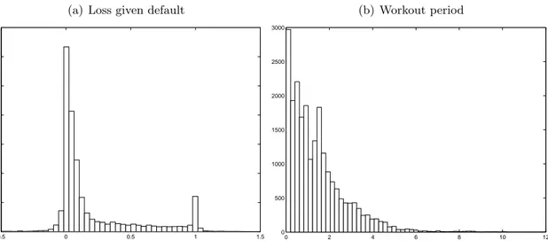
and Zagst (2007) and Hartmann-Wendels et al. (2014). Figure 1(a) presents the empirical LGD distribution, and shows that we can not ignore this, because over 10% of the LGDs lie outside the
[0,1] interval.
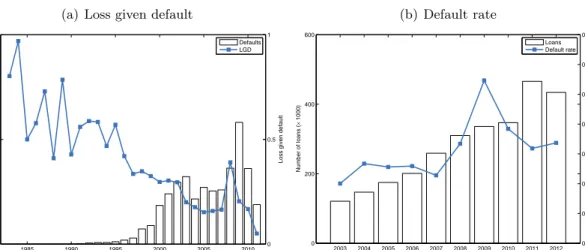
We restrict our analysis to the period 2003–2010. The LGD database for resolved defaults contains details of defaults from 1983 to 2014. Figure 2(a) shows the average LGD per year. The number of defaults in the database is small until the early 2000s and the average LGD is noisy because of it. The first defaults have been submitted by the banks in 2005. Not all banks might have databases with all relevant details of many years ago and most observations in the years before 2000 are the substantial losses with a long workout period still in the books.
The workout period is the main difference between bonds and bank loans. Bond holders directly 4
observe a drop in value as trading continues and the price is discounted by the expected recovery rate. For defaulted bank loans, a recovery process starts that should lead to debt repayment. When no more payments can be obtained, the default is resolved and the recovery process ends. The period from the default date to the resolved date is called the workout period. Most defaults are resolved within one to three years after default, but figure 1(b) shows that the recovery process can last more than five years.
Table I shows that the LGD is significantly higher for longer workout periods, which explains the high average LGD in figure 2(a) before 2003. The higher LGD for loans with longer workout periods is partly explained by discounting. The cash flows are discounted over a longer workout period, thus reducing the recovery and increasing the LGD. Additionally, the workout period is an indication of how hard it is to recover the outstanding debt. If the recovery takes time, it can be due to issues with restructuring or selling of the assets. If demand for an asset is high, it will be sold or restructured faster and its value will be higher.
The database only contains resolved defaults, for which the recovery process has ended, and therefore, by definition, the later years of the database (2011 to 2014) only contain defaults with shorter workout periods. Because a shorter workout period is related to a smaller LGD, the LGD is underestimated in the final years. The average LGD and number of defaults in 2011 is small compared to the previous years, see figure 2(a). Therefore, we restrict our analysis to the period 2003–2010.
Figure 2(b) shows the yearly default rate. In general, the default rate is relatively small with values mostly around 1%. The default rate increases during the financial crises, peaking in 2009 at a default rate of 2.2%, more than twice the default rate in the period 2003–2007. The figure shows that the total number of loans is large in 2003 and increases over time. This is mostly because the number of participating banks increases as well. To match the time period of the LGD dataset, we use the period 2003–2010.
The LGD sample after applying the sample selection consists of 22,080 observations of mostly European defaults, one of the most comprehensive datasets for bank loan LGD studied thus far. Grunert and Weber (2009) summarize the empirical studies on bank loan recovery rates. The largest dataset they found studies 5,782 observations over the period 1992–1995. More recently, Calabrese and Zenga (2010), Calabrese (2014a) and Calabrese (2014b) study a portfolio of 149,378
Italian bank loan recovery rates resolved in 1999 and Hartmann-Wendels et al. (2014) consider 14,322 defaulted German lease contracts from mainly 2001–2009. However, these studies focus on defaults from a single country or a single type whereas our dataset is more extensive.
[Figure 1 about here.] [Table 1 about here.] [Figure 2 about here.]
2.2 Sample Characteristics
In this section, we discuss the empirical LGD distribution, the pattern over time and differences across loan characteristics for our sample.
It is a stylized fact that LGD follows a bimodal distribution with most observations close to 0 or 1, see for example Schuermann (2004). In most cases, there is either no or a full loss on the default. Figure 1(a) shows that this also holds for our sample. By far most losses are close to 0,
but there is an additional peak at 1. The data is limited to the interval−0.5 to 1.5. Still, 12.52%
of the observations are outside the [0,1] interval.
In our analysis, defaults are aggregated per quarter to have both a sufficient number of time periods and a sufficient number of observations per period. An advantage of aggregation by quarter is that it matches the frequency of macroeconomic variables. Figure 2(a) shows the average LGD for defaults per quarter. The LGD starts with a relatively large value in 2003 and gradually decreases until 2007. From 2007, the average LGD increases due to the financial crisis. The level is back at its pre-crisis average in 2009. We observe the same pattern for the default rate in figure 2(b).
Figure 3 provides a more in-depth view of the time-variation of the LGD. It shows how the empirical distribution varies from quarter to quarter for the period 2003–2010. All quarters display the bimodal shape with peaks at 0 and 1. The increased number of defaults due to the financial crisis is visible, as well as the increase of the height of the peak around a LGD of 1 for the period 2007–2009. The large proportion of full losses explains the large average LGD in those years. Our modeling framework exploits both the bimodality of and the time-variation in the LGD.
Summary statistics of the sample and subsets based on loan characteristics are presented in table II. As expected, the LGD for unsecured loans is on average larger than for secured loans
because the former are not backed by collateral or a guarantor. Also, the average LGD is larger for subordinated loans than for senior loans. For some groups not many defaults are available. Therefore, we limit our analysis of groups to those with on average at least 100 observations per quarter.
Table II shows that unimodality is rejected by Hartigan and Hartigan’s (1985) dip test for the full sample as well as for subsamples, unless the number of defaults is small. The fraction of defaults with an LGD larger than 0.5 is reported to illustrate the close relation with the average LGD.
Because we want to compare multiple means and the LGD is not normally distributed, we use the Kruskal-Wallis (KW) test to test for differences in location of multiple distributions. The KW test is a nonparametric test based on ranks. It tests for the null hypothesis of identical distributions against the alternative of at least two distributions differing in location.
A KW test on the selected groups shows a significant difference between the senior secured and
senior unsecured loans, with a p-value of 0.000. Even though the absolute difference between the
average of SME and large corporate seems small, the p-value of the KW test is 0.000, strongly
rejecting the null hypothesis of equal distributions. For the industries, the LGD for financials is significantly larger than for the industrials and consumer staples industries.
[Figure 3 about here.]
[Table 2 about here.]
2.3 Macroeconomic Variables
Allen and Saunders (2003), Pesaran et al. (2006), Duffie et al. (2007), Azizpour et al. (2010), Creal et al. (2014) and others show that bond defaults are related to the business cycle. We include macroeconomic variables to analyze this behavior for bank loans. We consider the same set of variables as Creal et al. (2014) to represent the state of the economy: the gross domestic product (GDP), industrial production (IP) and the unemployment rate (UR). The series included are the growth compared to the same quarter in the previous year, seasonally adjusted. To match the mostly European default dataset, we use macro variables of European OECD countries or the European union.
3
Model specification
We propose a ‘mixed-measurement’ model (Creal et al., 2014), where the observations can follow
different distributions, but depend on the single latent factorαt. The latent factor follows an AR(1)
process,
αt+1 =γ+ραt+ηt, (1)
withηt∼N(0, ω2). The initial state α1 follows the unconditional distribution of the latent proces,
α1 ∼N γ/(1−ρ), ω2/(1−ρ2)
.
3.1 Loss given default
Based on the empirical distribution in figure 1(a), we propose a mixture of two normals for the
LGD and define distributions 0 and 1 as the distributions for good and bad loans,5
ylit∼ N µj0, σj2
ifsit= 0 (good loan),
N
µj1, σj2
ifsit= 1 (bad loan),
(2)
withyitl the LGD of loanithat defaulted at time tfori= 1, . . . , Nl,j= 1, . . . , J and t= 1, . . . T.
We treatsit as the unobserved state that is 1 if loaniat timetis a bad loan and 0 otherwise. The
probability that LGD is a bad loan varies across loan characteristics, such as industry or seniority, and across time. We define the sets of loans belonging to the categories of a loan characteristic as Cj for j = 1, . . . , J. For example, we have the categories large corporate and SME for loan
characteristic asset class. If the loan i defaulted at time t belongs to the category Cj, then the
probability of a bad loan is
P(sit= 1|i∈Cj) =pjt= Λ
βjl0+βjl1αt
, (3)
where Λ(x) = exp(x)/ 1 + exp(x)
is the logistic function. The model has one factorαt, such that
differences between groups are due to coefficients βjl0 and βjl1.
The distribution can change in three ways, influencing the average LGD: (i) a change in the 5
mixture probability P(sit = 1), (ii) a change in the mean of good loans µj0 and/or (iii) a change
in the mean of bad loansµj1. Most LGDs are (close to) 0 or 1, see figure 1(a), so we do not expect
the means to vary much. This is supported by figure 3, where the modes stay at 0 and 1, but the (relative) height of the peaks varies over time. Therefore, we propose that a larger (smaller) average LGD in a time period is caused by an increase (decrease) in the proportion of bad to good loans. We examine the alternative of time-varying means in section 7.2. We restrict the variance to
be equal across the mixture components for identification of the modes and µj0 < µj1 to interpret
good and bad loans.
3.2 Default rate
The default of loan i at time t follows a Bernoulli distribution. This implies that the number of
defaults in periodt is a realization of a binomial distribution, as in Bruche and Gonz´alez-Aguado
(2010). The distribution depends on the latent signal αt through the probability of defaultqit,
yitd ∼Binomial(Lit, qit), (4)
qit= Λ
βdi0+βid1αt
, (5)
withyitd the number of defaults andLit the number of loans of groupi at timet fori= 1, . . . , Nd
and t= 1, . . . T. If it is available from the DR database, we use the group specific default rate to
match the J groups in the LGD component, otherwise we use the full sample default rate. Hence,
Nd is either 1 or J, which is for example three for industries.
The defaults and loans are observed yearly, not quarterly. We set the third quarter equal to the yearly observation, because this is approximately the middle of year, and define the other quarters
as missing.6 Using the same method, Bernanke et al. (1997) construct a monthly time series from
a quarterly observed variable.
3.3 Macroeconomic variables
To relate the latent factor to the state of the economy, we add macroeconomic variables to the model,
ymt =βm0 +βm1αt+νt, (6)
where ym
t is the Nm×1 observation of the macro variables at time t and νt ∼ N(0,Σ) for t =
1, . . . , T. The macro variables are standardized to have zero mean and unit variance, such that we can easily compare the relation with the latent factor across the macro variables.
3.4 Missing values and identification
We do not observe multiple defaults per loan. We treat the loans for which the default date is not
in period tas missing during that quarter. For each loan, we have one observed andT−1 missing
values. One of the advantages of a state space model is its ability to easily handle missing values.
The densities are cross-sectionally independent given αt, such that
logp(yt|αt) =
N
X
i=1
δitlogpi(yit|αt), (7)
whereyt= (y1t, . . . , yN t)0,N =Nl+Nd+Nmis the number of observations andδit is an indicator
function which is 1 ifyitis observed and 0 otherwise. Therefore, only the observed values determine
the loglikelihood. The loglikelihood consists of the sum of the model components. The different components are given in appendix C.1.
Without restrictions, the latent factor α and the coefficients β0 and β1 are not identified. For
identification of β0, we set the interceptγ = 0 in equation (1). To make sure β1 is identified, we
standardize the signal variance ω2 = 1. Finally, we restrict one element of β
1 to be positive to
4
Estimation
Estimation of the parameters, denoted byθ, is done using maximum likelihood. Analytical solutions
are not available and direct numerical optimization is infeasible, due to the dimensionality of the
optimization problem. Because it would be possible to optimize for the parameters θ if α were
known and vice versa, we employ the Expectation Maximization (EM) algorithm, introduced by Dempster et al. (1977) and developed for state space models by Shumway and Stoffer (1982) and Watson and Engle (1983). The algorithm is a well-known iterative procedure consisting of repeating two steps, which is proven to increase the loglikelihood for every iteration.
The m-th iteration of the EM algorithm is
1. E-step: Given the estimate of the m-th iterationθ(m), take the expectation of the complete
data loglikelihood `c(θ|Y,S,α),
Q(θ|θ(m)) = Eθ(m)[`c(θ|Y,S,α)]. (8)
Evaluating the expected value of the complete data loglikelihood implies that we need
expected values for the statesSand the latent signalαgiven the observed LGD, defaults and
macro variables. Because the mixed-measurement model is a nonlinear non-Gaussian state space model, methods for linear Gaussian state space models like the Kalman filter are invalid. Following Jungbacker and Koopman (2007), we therefore apply importance sampling to get a
smoothed estimate of the expected value, variance and autocovariance ofα, the probability of
a bad loanP(sit = 1|Y,α) and its cross-product. We draw from an approximating Gaussian
state space model as importance density. Appendix B provides an outline of the method. The expected loglikelihood (8) is derived in appendix C.2 and C.3. Derivations for mode
estimation ofα, used to get the approximating Gaussian state space model, are in appendix
C.4. We set the number of replicationsR= 1000 and employ four antithetic variables in the
importance sampling algorithm. IncreasingR does not impact the results.
toθ,
θ(m+1) = arg max
θ
Q(θ|θ(m)). (9) Solving equation (9) involves the method of maximum likelihood. We use analytical solutions for the parameters if possible because the EM algorithm is already an iterative optimization.
That is, we numerically optimize ρ, βlj0 and βjl1 for j = 1, . . . , J, and βid0 and βid1 for i =
1, . . . , Nd, and use analytical solutions for the other parameters. The analytical solutions are conditional on the other parameters, which makes the two-step procedure an ECM algorithm (Meng and Rubin, 1993).
These steps are repeated until the stopping criterion is met. If the loglikelihood increase after the
m-th step, denoted by ` θ(m)|Y−` θ(m−1)|Y, is smaller than = 10−3, we switch to direct
numerical optimization of the loglikelihood until the loglikelihood increase is less than = 10−6.
Increasing the precision does not impact results.
Following Ho et al. (2012), we initialize the EM algorithm by 2-means clustering with random
starting values. Then, starting values forµj0andµj1are the sample mean of the two clusters andσj2
their average variance. We set Λ(βjl0) equal to the group proportions from 2-means clustering and
Λ(βid0) to the average default rate. Finally,βjl1 = 1 for allj= 1, . . . , J,βid1 = 1 for alli= 1, . . . , Nd,
and the factor is initialized at zero.
5
Results
5.1 LGD and DR
First, we discuss results for the model without cross-sectional variation, i.e. we do not use different factors or coefficients for groups such as industries or asset classes. The LGD parameter estimates are presented in the first column of table III.
The parameter estimates clearly distinguish two distributions. The estimate for the mean of a good loan is 0.072 and for the mean of a bad loan 0.828. The estimates for the means confirm our interpretation of the components as the distributions of good and bad loans and captures the stylized fact that most LGDs are either close to 0 or 1. The mean for bad loans is not exactly 1,
because of the observations between 0 and 1.7
We cannot directly compare the sensitivities towards the factor of LGD and the defaults via the
coefficients β1l and β1d because of the nonlinearity of the logistic function. Instead, we compare the
average marginal effect of the signal, given by the average of the first derivative of the probability
function with respect to the signal αt, 1/TPT
t=1∂pt/∂αt. We present these effects in panel F of
table III.
The coefficients βl
1 and β1d are both significantly positive, which means that the probabilities
of a bad loanpt and of a default qt move in the same direction. The significant effect of the factor
is strengthened by a large average marginal effect of 0.041 for pt, which means that a rise of the
factor by one standard deviation increases the probability of a bad loan by 4.1%. It indicates that the factor has a stronger effect on the probability of a bad loan than for the default probability,
where the effect is 1.2%, so pt fluctuates more than qt. They follow the same pattern over time,
but at a different level, see figure 4. This is in line with research on losses on bonds, where DR and LGD are time-varying through a common cyclical component.
The factor underlying the probability of a bad loan is presented in figure 4(a). Due to
the monotonicity of the logistic transformation, interpreting the factor and its coefficients is
straightforward. The positive estimate for βl1 means that an increase of the factor corresponds
with an increase in the ex ante probability of a bad loan and a default.
The estimated factor resembles the average LGD. The first few years are characterized by a downward trend until 2007. In 2007 the level increases, after which in 2009 it decreases slightly. It differs however, for a couple of reasons. First, the factor is a combination of the LGD, the default rates and macroeconomic variables and is estimated using all three sources of information. Second, the factor is a smoothed estimate, which means that it is conditional on all information of the complete sample period. It is not simply the average of the LGD at the particular point in time, but contains information from the preceding and following observations.
Figure 5 shows the fit of the mixture for two quarters. The difference between the two panels
is the ex ante probability of a bad loanpt, which is larger in the second quarter of 2008, such that
7
To fit the observations between the modes, the means are shrunk to 0.5. The shrinkage is stronger forµ1because
the number of observations with an LGD near 1 is smaller than the number of defaults with an LGD near 0, see figure
5. The estimates of the means are closer to 0 and 1 if we replace the mixture of normals by a mixture of Student’st
the relative height of the mode for bad loans compared to good loans is higher. The relatively high mode for bad loans corresponds with the relatively large fraction of high LGD observations in the second quarter of 2008. Further, for both quarters, the location of the distribution of good loans captures the large peak at 0 and the distribution of bad loans fits the high LGD observations. It captures the stylized fact and the changes across time match what we observe in the empirical distribution.
Similar to losses on bonds, the defaults show cyclical behavior. Higher default rates are
accompanied by a higher probability of a bad loan, hence aggravating the loss during bad times. This time-variation should be taken into account. The claim that LGD estimates should “reflect economic downturn conditions where necessary to capture the relevant risks” (BCBS, 2005) is mostly motivated by research on bonds. We provide evidence that it holds for bank loans as well.
[Table 3 about here.]
[Figure 4 about here.]
[Figure 5 about here.]
5.2 Relation with Macroeconomic Variables
Research on losses on bonds reports a link with macroeconomic variables, see e.g. Allen and
Saunders (2003). Here, we investigate this link for losses on bank loans. The coefficients in panel D of table III indicate a relation between the state of the economy and credit conditions. They are significantly different from zero and have the expected sign. GDP and IP are negatively related, whereas the UR is positively related to the factor. Because a high factor implies more bad loans and a high default rate, this finding implies that both the number of defaults and the proportion of bad loans increase when the economy is in a bad state.
The first two columns of table III and figure 6 show that including the macro variables alters the factor only slightly. The factor of the model with macro variables in figure 6 is almost identical to the factor of the model without macro variables: the correlation between both factors is 0.996. Further, the coefficients of the LGD and DR only vary slightly. The macro variables support the shape of the factor we find, but do not drive the results.
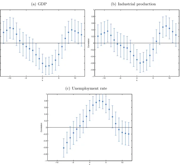
The model includes contemporaneous macro variables, but the actual relation between the economy and the credit conditions may exhibit leading or lagging behavior. On the one hand, it could be that if the economy deteriorates, it takes a few months before companies are affected and go into default. On the other hand, the default of many companies could turn the economy into distress. The workout period further distorts the relation. The LGD are grouped by default date, but are a combination of cash flows in the recovery period, which depend on the state of the economy during the recovery period. The workout period can be less than a year or take up to five years.
Figure 7 presents the correlation of the factor for the model with default rate and macro variables with the macroeconomic variables for different leads and lags. The correlations with both GDP and IP show that the factor is contemporaneously related to the state of the economy. The unemployment rate is strongly related to the factor lagged three or four periods, in line with the other correlations because UR lags the state of the economy. Figure 7 confirms the significant relation we find from the estimates in table III, but also shows that the link between macro variables and credit conditions is more complicated than indicated by the model.
[Figure 6 about here.]
[Figure 7 about here.]
5.3 Loan Characteristics
We expect differences in credit conditions across loan characteristics, such as seniority and industry. We examine two possibilities: (i) one factor is underlying all groups, but the parameters vary depending on the characteristics, or (ii) every category has a different underlying factor. The first model type implies that the underlying credit conditions change in the same way for all industries, but the sensitivities towards it can vary. The second model type allows for different credit cycles per group. Under this model type, it could be that industry A is in distress, whereas the credit conditions in industry B are not irregular. We investigate how related the group-specific credit conditions are. If there are differences, banks can exploit this to diversify their portfolio. The characteristics we look into are security, seniority, asset class and industry, but only select categories with on average at least 100 observations per quarter. For the different asset classes and industries,
we use group-specific default rates. Macro variables are included to compare the relation with the business cycle.
The parameter estimates for the first model type, with a single common factor for all groups, are presented in the first column in tables IV–VI. The parameter estimates for the second model type, with a different latent factor per group, are presented in the remaining columns. The main
differences in LGD across groups are the coefficients βjl0 and βlj1, which determine the relation
between the factor and the probability of a bad loan. The identification of the distributions of good and bad loans holds for all subsamples. The means for good loans are estimated between 0.05 and 0.09 and for bad loans between 0.79 and 0.86.
First, consider the difference between senior secured and unsecured loans in table IV. The
intercept βjl0 is more negative for senior secured loans than for unsecured loans which means that
the average LGD is smaller for secured loans. The average marginal effect is almost twice as high for senior secured loans than for unsecured loans, which implies a higher sensitivity for the
time-variation in the latent factor. This is reflected in the high estimate for βjl1 for senior secured
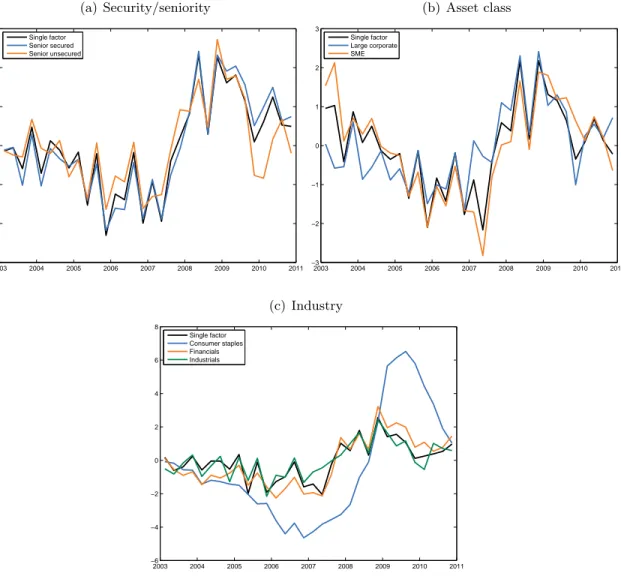
loans. Figure 8(a) shows that the pattern over time is much alike for the for the senior secured and unsecured factors. The correlation between the factors is 0.84. The finding that senior secured defaults are more time-varying than unsecured defaults is in contrast with the findings of Araten et al. (2004). An explanation is that the values of the securities backing the loan are cyclical. For example, demand for the collateral may vary depending on the state of the economy and its value therefore changes substantially over time.
Second, we consider the asset classes large corporate (LC) and small and medium enterprises (SME), where we have group-specific default rates. Table V presents the parameter estimates. If we consider different factors per group, the mean marginal effect for the LGD is approximately the same. However, the factor for SME is more connected with macroeconomic conditions. In particular the difference in the relation with UR is substantial, see panel D of table V. Given the
estimates of βjl0, βjl1 and the average marginal effect in the model with one common factor, the
LGD for SME loans is slightly higher and more sensitive to changes in the factor. In contrast, the
mean marginal effect for the default rate of LC is much higher than for SME. The estimate forβjd0
is higher for LC than for SME, which implies that bank loans on LC default relatively more often. The time-variation of credit conditions for asset classes LC and SME differs in pattern and
in size. The correlation between the factors for LC and SME in figure 8(b) is only 0.59. The LGD for SME is slightly more time-varying than for LC, but the default rate for LC is much more time-varying than for SME.
Third, we study the difference in cyclicality across industries, for which we also have the industry-specific default rates. Consumer staples (CS) should be an industry with relatively stable credit conditions over time, because it produces goods such as food and household supplies. Demand will exist, independent of the economic situation. On the other hand, financials (FIN) are expected to be volatile, especially because the time period includes the financial crisis of 2007–2009.
The estimate of coefficient βjl1 in table VI is largest for FIN, which induces the high mean
marginal effect of 0.049. As expected, the LGD for FIN is most sensitive to changes in the factor.
The estimate of βjl0 is smaller than that of the other industries. Hence, the probability of a bad
loan is in general smaller for FIN, but more sensitive to economic conditions. The time-variation explains the significantly larger average LGD over the full sample in section 2.2.
If we consider industry-specific factors, the mean marginal effect is smallest for CS, both for the
LGD and the default rate. The estimates for the coefficients βl
j1 and βjd1 are both approximately
0.05 in the second column of table VI. If we allow for a single factor, the mean marginal effects are larger, but still small compared to FIN.
For industrials (IND), the LGD is less time-varying compared to other industries. The estimate
of βjl1 for the model with a single factor is smaller than for CS. If all industries have a different
factor, the time-varying effect is stronger for IND. On the other hand, the default rate is sensitive to credit conditions. The default rate has the highest mean marginal effect for IND, slightly higher than for FIN, in both the model with an industry-specific factor and the model with a single factor. The difference between industries is further illustrated by the relation with the macroeconomic variables. Panel D of table VI shows that the factor underlying the industries FIN and IND is closer related to the macroeconomic variables than for CS. The coefficients for GDP and IP are estimated almost twice as high for FIN and IND. The credit conditions of CS are less related to the macroeconomic variables than for the other industries.
Figure 8(c) presents the single factor and the industry-specific factors. The industry factors move in the same direction over time, as the recent crisis hit all of the considered industries. But they are far from identical, with correlations from 0.52 between the factors of CS and IND to 0.81
between those of FIN and IND. The response of the factor of CS is lagged, but stronger than for the other industries. The increase of the factor of CS is larger than for other industries, but the mean marginal effect on the probability of a bad loan is only 0.007. This is due to the small estimate for
the coefficient βjl1.
The results indicate that it is important to consider the portfolio composition of defaults. We find that there is not a single credit cycle. The credit conditions across loan characteristics do share a common component, but clear differences exist. The probability of a bad loan determines most variation across groups, in terms of level and time-variation. Senior secured loans vary more over time, whereas unsecured loans have a higher average probability of a bad loan. Especially the time-variation across industries is important for banks focusing on a small set of sectors. Financials are sensitive to macro conditions, while consumer staples are more stable over time.
Banks gain a more in-depth view of the risk of the loan portfolio and how sensitive it is to macro conditions by taking the loan characteristics into account. For example, they can anticipate industry-specific time-variations and adjust their risk parameters accordingly to more accurately
estimate the loan-specific risk. Further, they can diversify some of their time-varying risk by
investing in different industries or asset classes.
[Table 4 about here.]
[Table 5 about here.]
[Table 6 about here.]
[Figure 8 about here.]
5.4 Relation with Financial Variables
The latent factor underlies both the default rates and the loss given default. Therefore, we interpret the factor as a measure for credit conditions and we expect it to have a relation with other financial
variables. We examine this by adding financial variables to the vector ymt in equation (6). We
select the long-term interest rate (LIR), the credit spread (CRS) and the yield spread (YLS). The LIR is the yield on the Euro area 10-years government bond, the CRS is the difference between the yield on the IBOXX European corporate 10+-years BBB-rated bond index and the LIR, and the
YLS is the difference between the LIR and the yield on the 3-month Euro Interbank Offered Rate (Euribor).
The last column of table III presents the estimates of the model including the financial variables. The estimates in panel E of table III indicate a significant positive relation between the factor and the financial variables. In particular, we observe a strong connection with the credit spread, given
the estimate of 0.578 for β1m. This strong connection is not surprising, because the credit spread
represents the market’s expectation of credit risk, in terms of default rate and LGD.
Further, adding the financial variables does not affect the relation of the LGD, defaults and macro variables with the factor. The latent factor is virtually unchanged with a correlation of 0.997 with the factor from the model without financial variables.
The results validate our interpretation of the factor for credit conditions given the strong relation with the credit spread.
6
Applications in Risk Management
Banks can apply the model to assess their risks. The model can be used in a stress testing exercise or to formulate a downturn LGD (see e.g. Calabrese, 2014a). Below, we illustrate its use to determine economic capital and show how we can predict future credit conditions.
6.1 Economic Capital
Economic capital is an internal risk measure used by banks. It represents the amount of capital that the bank should hold in order to remain solvent, accounting for unexpected losses due to their exposure to risks. Given an estimate for the latent factor, we simulate realizations of defaults and LGD. In particular, it yields the economic capital, which is computed as the difference between the loss at a particular quantile in the right tail, usually at 99.9%, and the expected loss. For a given loan portfolio, based on simulated losses, we get the corresponding loss distribution.
We draw 50,000 times for every time period a portfolio of 2,000 loans, each with an exposure
at default (EAD) of e1, similar to the portfolio considered by Miu and Ozdemir (2006) in their
simulation exercise. Further, we consider the latent factor distributed as the one inferred in section 5.1, from the model including macro variables but without differences per group, such that we do
not have to make assumptions on the portfolio composition over industry and asset class.
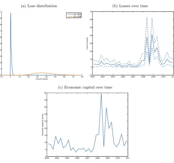
The results show that changes in credit conditions can have severe consequences for the portfolio loss. First, figure 9(a) shows the loss distribution for two quarters. The two distributions are clearly different, only due to a difference in credit conditions, given by the level of the latent factor. In the fourth quarter of 2005, when the factor is low (see figure 4(a)), most losses are (close to) 0 and barely exceed 0.25% of the loan amount. On the other hand, in the second quarter of 2008, when the factor is high, the losses are more dispersed and almost always larger than 1% of the loan amount.
Figure 9(b) presents the loss distribution over time, and confirms the vast differences in loss distribution. The expected loss is mostly between 0% and 0.25% of the loan amount, but increases to 2% in 2008. The entire 95% confidence interval of losses in the second and fourth quarter of 2008 is larger than the maximum loss of the 95% interval for the period up to 2008, and 2010.
Finally, figure 9(c) presents the economic capital at 99.9% over time and shows that the right tail becomes fatter during bad credit conditions. The economic capital varies much over time with a maximum of 2.23% of the loan amount, approximately 15 times the minimum of 0.15%. Ignoring the fluctuation induces large uncovered potential losses.
An advantage of our model is its easy adaptation to a specific portfolio, the composition of loans over asset class, industry or other characteristics, because we can distinguish between different groups as in section 5.3. The loss distribution and economic capital varies per portfolio and sampling from a more tailored portfolio yields a more accurate loss distribution. Using a tailored model yields insight in the bank’s risk and how it changes by adjusting the strategy, moving in or out a particular sector.
[Figure 9 about here.]
6.2 Prediction
The previous section shows that we can calculate the economic capital based on simulations for the estimation period, using information on the resolved defaults. It takes some time before all defaults are resolved and the economic LGD is observed. Due to the workout period, the estimation period excludes the most recent years, see section 2.1. We would like to have information on the losses on
the unresolved defaults that occurred in the recent years, and predict future losses. Banks can form an expectation of the write-offs for unresolved defaults and construct scenarios for future credit conditions. In this section, we propose two methods to predict future credit conditions, such that we can determine the economic capital out-of-sample.
The first method predicts the factor based on the autoregressive process in equation (1), such
that the factor predicted h periods ahead is given by αT+h|T = ρhαT|T. A disadvantage of this
method is that it ignores the available information in the recent years. The prediction of the factor
at timeT+h, for forecast horizonh >0, is only based on the information in the estimation period,
the period up to timeT.
A second method uses the information available in the out-of-sample period. For example, we can use the macroeconomic information to update the prediction of the latent factor. An advantage of using macro variables is that they are reported quarterly, whereas credit data such as the default rate is usually only available at the end of the year. Another advantage is that if we only use the macro variables, the model reduces to a linear Gaussian state space model and we can apply straightforward methods such as the Kalman filter to update the prediction.
The method involves updating the prediction of the factor at timeT+hto get a filtered estimate,
based on the information up to time T +h. The factor estimate from the autoregressive process
at each one-step ahead forecast is adjusted based on the prediction error for the macroeconomic variables, given the relation in equation (6).
We compare both prediction methods by considering the out-of-sample period 2011–2013, for which macro information is available. Figure 10(a) shows that using the macro information strongly
decreases the variance of the forecasted factor. For period T + 1, the first quarter of 2011,
the variance of the filtered factor is only 56% of the variance of the predicted factor, based on
information up to and including 2010, timeT. Further, the credit conditions are forecasted to be
worse, whereas we cannot infer anything on the direction of the factor from the prediction based on information without out-of-sample macro information. The prediction of the first method is not far from the long-run average partly because the factor is already close to 0 at the end of the
in-sample period. The prediction starts at the level of the factor at time T and converges to the
long-run average with the rate of the AR coefficientρ as the forecast horizon increases.
each with an EAD ofe1, simulated 50,000 times. The economic capital at 99.9% increases quickly with the forecast horizon if the macro information is ignored, due to the added uncertainty. On the other hand, if the macro information is taken into account, the economic capital does not explode. The variance of the filtered estimate does not increase with the forecast horizon, such that the difference in economic capital is only due to a change in the level of the factor.
Alternatively, we could have included financial variables, such as the credit spread, yield spread and long-term interest rate from section 5.4. Macro variables are reported with a lag, whereas the financial variables are available instantaneously and can be used to predict in real time. Further, we could include lagged macro variables such that the information we need to predict the credit
conditions at time T+ 1 is available at timeT.
[Figure 10 about here.]
7
Alternative Specifications
The current model for LGD proposes time-variation in the probability of a bad loan in a mixture of normals. In this section, we challenge the proposed model by considering alternative specifications. First, we test whether the distribution is time-varying and consider time-varying means to introduce
time-variation into the mixture. Second, we check whether a mixture of Student’s t distributions
provides a better fit.
7.1 No Time-Variation
To test whether the time-variation is present in our sample, we estimate a mixture of normals on the full set of LGD observations using a standard EM algorithm for mixtures.
The results in table VII confirm that the probability of a bad loan is time-varying. The large difference in loglikelihood provides significant evidence of time-variation in our LGD sample. Even if we account for the larger number of parameters, the model where the probability of a bad loan can vary over time provides a better fit in terms of BIC. Hence, this time-variation should be taken into account when constructing LGD estimates.
7.2 Time-Variation in the Mean
The model for the LGD includes a time-varying probability of a bad loan. Here, we introduce time-variation through the mean of a good or bad loan. We replace equations (2) and (3) by a
mixture of normals withP(sit = 1) =pand µ0t=µ0+β1lαtand/or µ1t=µ1+β1lαt. To estimate
the parameters and the latent factor, we combine the state space methods for dynamic linear models of Shumway and Stoffer (1991) and the univariate treatment of Durbin and Koopman (2012). The univariate treatment can be applied because the observations are independent conditional on the latent factor.
First, table VII shows that the parameter estimates for β1l are very small. This indicates that
the time-varying aspect in the means is not important. Second, table VII shows that the models with time-varying mean are barely able to improve the fit in terms of loglikelihood, and are even worse compared to the model without time-variation when accounting for the increased number of parameters. Third, figure 6 shows that models with (one of) the means time-varying underestimate the observed time-variation in the average LGD. The difference with the sample average is almost 0.1 on a scale of 0 to 1 during very good or bad times. An error of this size on the LGD leads to under- or overestimation of the expected losses on a portfolio, especially during times when it matters most. Only the model with time-varying probability of a bad loan is able to replicate the pattern of the average LGD over time.
These results confirm that the time-variation is due to changes in the probability of a bad loan, and not due to shifts of the location of the distributions.
[Figure 11 about here.]
7.3 Mixture of Student’s t Distributions
To test whether a different distribution than the normal provides a better fit, we replace the mixture
of normals in equation (2) by a mixture of Student’stdistributions. The probability of a bad loan
remains time-varying. To estimate the parameters and the latent factor, we use the ECM algorithm
of Basso et al. (2010)8in combination with the importance sampling methods described in appendix
B.
The last column of table VII presents the parameter estimates. The peaks of the empirical distribution are better identified compared to the mixture of normals with means equal to 0.03 and 0.99. The fit is improved, as reflected in a higher loglikelihood. Figure 12 shows the fit for the same quarters as figure 5 and clearly illustrates that the empirical distribution is described better by a
mixture of Student’st distributions. Not only the location, but also the peakedness of the modes
is captured. The improved identification could imply a more accurate estimate of the probability of a bad loan and the latent factor. However, figure 13 shows that the factor is largely unaffected by changes in distribution. The correlation between the factor with a mixture of normals and the
factor from the model with a mixture of Student’s tdistributions is 0.99.
Using the model with the Student’s tdistribution comes with some disadvantages. Due to the
large peakedness at 0 and 1 and the observations between the modes, the degrees of freedom are estimated close to 1 for good loans and even below 1 for bad loans. None of the moments are
defined for a distribution with less than 1 degree of freedom, which makes it difficult to interpretµ0
and µ1. Further, a default observed with an LGD larger than 1 could be identified as a good loan
by the model, although it clearly is not because more than the full exposure is lost. Figure 14(b)
shows that this happens because the smoothed probabilities of a bad loan ˆπit =P(sit = 1|ylit, αt)
decrease (increase) for LGD values larger (smaller) than the mean of the distribution of bad (good) loans due to the fat tails. None of the issues occur if we use the mixture of normals, see figure 14(a).
The model with the mixture of normals is preferred over the mixture of Student’stdistributions.
Even though the model with the fat-tailed distribution provides a better fit, it is difficult to interpret due to the low degrees of freedom and because some loans are obviously misidentified by the model. Further, the gains in terms of identification of the latent signal are limited, because the factor is very similar to a specification with a mixture of normals.
[Figure 12 about here.]
[Figure 13 about here.]
8
Conclusion
The loss given default and the default rate on bank loans are both cyclical. We infer a common underlying factor that is a measure for the credit conditions and related to the business cycle. The time-variation in the loss given default is explained by changes in the probability of a bad loan. Banks should take this into account when determining the risk parameters.
We propose a model that describes the stylized facts of the loss given default on bank loans well. It captures the bimodal shape of the empirical distribution and provides an interpretation of the components, by explicitly modeling the extremes of no and full loss. It is flexible enough to include the differences across loan characteristics that we find. Further, the model has applications in risk management, such as the calculation of the economic capital and the prediction of future credit conditions.
References
Allen, L. and Saunders, A. (2003). A survey of cyclical effects in credit risk measurement models. BIS Working Paper 126, Bank of International Settlements, Basel, Switzerland.
Altman, E., Brady, B., Resti, A., and Sironi, A. (2005). The Link between Default and Recovery
Rates: Theory, Empirical Evidence, and Implications. The Journal of Business, 78(6):2203–2228.
Araten, M., Jacobs, Jr., M., and Varshney, P. (2004). Measuring LGD on Commercial Loans: An
18-Year Internal Study. The RMA Journal, pages 28–35.
Azizpour, S., Giesecke, K., and Schwenkler, G. (2010). Exploring the Sources of Default Clustering. Technical report, Stanford University working paper series.
Basel Committee on Banking Supervision (2005). Guidance on Paragraph 468 of the Framework
Document. Bank for International Settlements.
Basso, R. M., Lachos, V. H., Cabral, C. R. B., and Ghosh, P. (2010). Robust mixture modeling
based on scale mixtures of skew-normal distributions. Computational Statistics & Data Analysis,
54(12):2926–2941.
Bernanke, B. S., Gertler, M., and Watson, M. W. (1997). Systematic Monetary Policy and the
Effects of Oil Price Shocks. Brookings Papers on Economic Activity, (1):91–157.
Bruche, M. and Gonz´alez-Aguado, C. (2010). Recovery rates, default probabilities, and the credit
cycle. Journal of Banking & Finance, 34(4):754–764.
Calabrese, R. (2014a). Downturn Loss Given Default: Mixture distribution estimation. European
Journal of Operational Research, 237(1):271–277.
Calabrese, R. (2014b). Predicting bank loan recovery rates with a mixed continuous-discrete model.
Applied Stochastic Models in Business and Industry, 30(2):99–114.
Calabrese, R. and Zenga, M. (2010). Bank loan recovery rates: Measuring and nonparametric
Creal, D., Schwaab, B., Koopman, S. J., and Lucas, A. (2014). Observation Driven
Mixed-Measurement Dynamic Factor Models with an Application to Credit Risk. Review of
Economics and Statistics, 96(5):898–915.
De Jong, P. and Shephard, N. (1995). The simulation smoother for time series models. Biometrika,
82(2):339–350.
Dempster, A. P., Laird, N. M., and Rubin, D. B. (1977). Maximum Likelihood from Incomplete
Data via the EM Algorithm. Journal of the Royal Statistical Society, 39(1):1–38.
Duffie, D., Saita, L., and Wang, K. (2007). Multi-period corporate default prediction with stochastic
covariates. Journal of Financial Economics, 83(3):635–665.
Durbin, J. and Koopman, S. J. (2012). Time series analysis by state space methods. Oxford
University Press.
Grunert, J. and Weber, M. (2009). Recovery rates of commercial lending: Empirical evidence for
German companies. Journal of Banking & Finance, 33(3):505–513.
Hartigan, J. A. and Hartigan, P. M. (1985). The Dip Test of Unimodality. The Annals of Statistics,
13(1):70–84.
Hartmann-Wendels, T., Miller, P., and T¨ows, E. (2014). Loss given default for leasing: Parametric
and nonparametric estimations. Journal of Banking & Finance, 40:364–375.
Ho, H. J., Pyne, S., and Lin, T. I. (2012). Maximum likelihood inference for mixtures of skew
Student-t-normal distributions through practical EM-type algorithms.Statistics and Computing,
22(1):287–299.
H¨ocht, S. and Zagst, R. (2007). Loan Recovery Determinants - A Pan-European Study. Working
Paper.
Jungbacker, B. and Koopman, S. J. (2007). Monte Carlo estimation for nonlinear non-Gaussian
state space models. Biometrika, 94(4):827–839.
Knaup, M. and Wagner, W. (2012). A Market-Based Measure of Credit Portfolio Quality and
Meng, X.-L. and Rubin, D. B. (1993). Maximum likelihood estimation via the ECM algorithm: A
general framework. Biometrika, 80(2):267–278.
Miu, P. and Ozdemir, B. (2006). Basel Requirement of Downturn LGD: Modeling and Estimating
PD & LGD Correlations. Journal of Credit Risk, 2(2):43–68.
Pesaran, M. H., Schuermann, T., Treutler, B.-J., and Weiner, S. M. (2006). Macroeconomic
Dynamics and Credit Risk: A Global Perspective. Journal of Money, Credit and Banking,
38(5):1211–1261.
Prates, M. O., Lachos, V. H., and Cabral, C. R. B. (2011). mixsmsn: Fitting Finite Mixture of
Scale Mixture of Skew-Normal Distributions. R package version 0.2-9.
Schuermann, T. (2004). What Do We Know About Loss Given Default? In Shimko, D., editor,
Credit Risk Models and Management, chapter 9. Risk Books, London, 2nd edition.
Shumway, R. H. and Stoffer, D. S. (1982). An Approach to Time Series Smoothing and Forecasting
using the EM Algorithm. Journal of Time Series Analysis, 3(4):253–264.
Shumway, R. H. and Stoffer, D. S. (1991). Dynamic Linear Models with Switching. Journal of the
American Statistical Association, 86(415):763–769.
Watson, M. W. and Engle, R. F. (1983). Alternative algorithms for the estimation of dynamic
Appendix A
Data Filter
Following H¨ocht and Zagst (2007), who also use data from the Global Credit Data Consortium,
and NIBC’s internal policy, we apply the following filters to the LGD database.
• EAD≥e100,000. The paper focuses on loans where there has been an actual (possible) loss, so EAD should be at least larger than 0. Furthermore, there are some extreme LGD values
in the database for small EAD. To account for this noise, loans with EAD smaller than e
100,000 are excluded.
• −10% < (CF +CO)−(EAD−EAR)
/(EAD+PA) < 10%, where CF cash flows, CO charge-offs and PA principal advances. The cash flows that make up the LGD should be plausible, because they are the major building blocks of the LGD. A way of checking this is by looking at under-/overpayments. The difference between the EAD and the exposure at resolution (EAR), where resolution is the moment where the default is resolved, should be close to the sum of the cash flows and charge-offs. The cash flow is the money coming in and the charge-off is the acknowledgement of a loss in the balance sheet, because the exposure is expected not to be repaid. Both reduce the exposure and should explain the difference between EAD and EAR. There might be an under- or overpayment, resulting in a difference. To exclude implausible cash flows, these loans are excluded when they are more than or equal to 10% of the EAD and principal advances (PA). The 10% is a choice of the Global Credit Data Consortium.
• −0.5≤ LGD ≤1.5. Although theoretically, LGD is expected between 0 and 1, it is possible
to have an LGD outside this range, e.g. due to principal advances or a profit on the sale of assets. Abnormally high or low values are excluded. They are implausible and influence LGD statistics too much.
• No government guarantees. The database contains loans with special guarantees from the government. Most of the loans are subordinated, but due to the guarantee, the average of the subordinated LGD is lower than expected. Because the loans are very different from others with the same seniority and to prevent underestimation of the subordinated LGD, these loans are excluded from the dataset.
Some consortium members also filter for high principle advances ratios, which is the sum of the principal advances divided by the EAD. Even though high ratios are plausible, they are considered to influence the data too much and therefore exclude loans with ratios larger than 100%. NIBC does include these loans, because they are supposed to contain valuable information and the influence of outliers is mitigated because they cap their LGD to 1.5. The data shows that the principal advances ratio does not exceed 100%, so applying the filter does not affect the data and is therefore not considered.
Appendix B
Importance Sampling
We outline the simulation based method of importance sampling, which we use to evaluate the non-Guassian state space model. For more information on importance sampling for state space models, see for example Durbin and Koopman (2012).
Consider the following nonlinear non-Gaussian state space model with a linear and Gaussian signal,
yt∼p(yt|αt), (10)
αt+1 =ραt+ηt, (11)
with ηt ∼NID(0, ω2) for t= 1, . . . , T, where yt is an N ×1 observation vector and αt the signal
at timet. For notational convenience, we express the state space model in matrix form. We stack
the observations into an N ×T observation matrix Y = (y1, . . . ,yT)0 and T ×1 signal vector
α= (α1, . . . , αT)0 such that we have
Y ∼p(Y|α), (12)
α∼N(µ,Ψ). (13) The method of importance sampling is a way of evaluating integrals by means of simulation.
It can be difficult or infeasible to sample directly fromp(α|Y), which is the case for non-Gaussian
state space models. Therefore, an importance density g(α|Y) is used to approximate the p(α|Y)
the functionx(α), ¯ x=E[x(α)|Y] = Z x(α)p(α|Y)dα= Z x(α)p(α|Y) g(α|Y)g(α|Y)dα=Eg x(α)p(α|Y) g(α|Y) . (14)
For a non-Gaussian state space model with Gaussian signal, this can be rewritten into
¯ x= Eg[x(α)w(α,Y)] Eg[w(α,Y)] , (15) w(α,Y) = p(Y|α) g(Y|α), (16)
which contains densities that are easy to sample from. Then ¯x is estimated by replacing the
expectations with its sample estimates.
The function to be estimatedx(α) can be any function ofα. For example, the mean is estimated
by settingx(α) =α. For the estimation of the likelihood L(θ|Y) =p(Y|θ) we have
L(θ|Y) =
Z p(α,Y)
g(α|Y)g(α|Y)dα=g(Y)
Z p(α,Y)
g(α,Y)g(α|Y)dα=Lg(θ|Y)Eg[w(α,Y)], (17)
where Lg(θ|Y) = g(Y) is the likelihood of the approximating Gaussian model. This is
estimated by the sample analog ˆLg(θ) ¯w, with ¯w = (1/R)PR
r=1w(α(r),Y) where α(r), r =
1, . . . , R, are independent draws from g(α|Y), using the simulation smoother. Its log version
is log ˆL(θ|Y) = log ˆLg(θ|Y) + log ¯w.
B.1 Mode Estimation
The importance density g(α|Y) must be chosen such that it is easy to sample from and
approximates the target density well. If the importance density does not share the support of the target density, the estimation will be inaccurate. An example of a suitable importance density is to take a Gaussian density that has the same mean and variance as the target density.
It is possible to sample from p(α|Y) for a Gaussian state space model using the simulation
smoother developed by De Jong and Shephard (1995). Therefore, we would like to get a Gaussian model that approximates the non-Gaussian model, defined by equations (10) and (11).