Optimized Memory Access For Dynamically Scheduled High Level Synthesis

OPTIMIZED MEMORY ACCESS FOR

DYNAMICALLY SCHEDULED

HIGH LEVEL SYNTHESIS

Submitted on the 29th of June, 2018 in part fulfillment of the

requirements for the degree of

Master of Computer Science

at the

Laboratoire d’architecture des processeurs (LAP)

of the

School of Computer and Communication Sciences,

École Polytechnique Fédérale de Lausanne (EPFL)

by

Atri Bhattacharyya

supervised by

Prof. Paolo Ienne, Director, LAP

Acknowledgements

I would like to thank my supervisor, Prof. Paolo Ienne, for the opportunity to do my Master’s project in the fascinating field of computer architecture and to be part of the intellectually stimulating and pleasant environment at the Laboratoire d’architecture de processeurs (LAP). His guidance during this project has been invaluable and his insistence on formally expressing concepts has been essential for me to get a clear grip on my own ideas.

My sincerest gratitude also goes out to Lana Josipovic whose doctoral research has been the basis for this project. She been around to help me at every stage of the way by suggesting paths to explore, acting a sounding board for my ideas and by critically reviewing all my work including the dreary exercise of proofreading this document. I would also like to acknowledge Andrea Guerrieri for helping me out with technical problems with the compiler infrastructure that threatened to derail the entire project at one point.

Most of all, I must thank my parents who have supported me through all of my endeavors irrespective of the odds. Without their love and unconditional support, none of this would have been possible. I am also grateful to my brother and cousins who have always been available to pump up drooping spirits. Together, they have been my pillars through thick and thin.

Finally, I would like to thank the staff at LAP and the School of Computer and Communication Sciences for helping me with all the associated formalities and for enabling me to work free of all hassles.

Abstract

Dynamically-scheduled elastic circuits generated by High-Level Synthesis (HLS) tools are inherently out-of-order, following the flow of data rather than the evolution of an instruc-tion pointer. Components of the circuit which access memory need to be connected to a Load-Store Queue (LSQ) that dynamically checks for memory dependencies, performs store ordering and forwarding, and allows unordered access to Random-Access Memory (RAM) whenever possible. While connecting every memory access (load/store) component to an LSQ ensures correctness of program execution, the hardware and power cost makes this solution unattractive. Statically ruling out dependencies allows circuits to access memory via lightweight components that use an arbitrator to handle RAM port sharing. Reducing the number of components using the LSQ allows the compiler to generate smaller queues which results in superlinear savings in hardware and power for the memory subsystem.

This work describes additions to the Elastic Compiler (EC) that allow it to analyze algorithms expressed in LLVM-IR, an intermediate code representation, to rule out memory dependen-cies between load/store instructions and their underlying insights. These analyses leverage pointer analysis as well as array access patterns to narrow down the list of possibly dependent instructions. We also enhance the compiler to leverage our analyses and automatically gener-ate relevant memory-access components for the circuit and to connect them to the relevant arbitrator or LSQ.

Contents

Acknowledgements iii

Abstract v

Introduction 1

1 Background 3

1.1 High Level Synthesis . . . 3

1.2 Scheduling and Elastic Circuits . . . 3

1.3 LLVM . . . 4

1.3.1 Pass Infrastructure . . . 6

1.4 Integer Polyhedra . . . 7

1.4.1 Integer Set Library . . . 7

1.5 Polly . . . 10

1.5.1 Static Control Parts . . . 10

1.5.2 ScopInfo Pass . . . 10

1.6 Elastic Compiler . . . 13

2 Memory Dependencies in Elastic Circuits 15 2.1 Elastic compiler: Memory access . . . 15

2.2 Architecture . . . 17

3 TokenDependenceInfo 19 3.1 Properties . . . 20

3.2 Proofs of properties . . . 22

3.3 Finding dependence relations . . . 22

3.3.1 Dependence . . . 24

3.3.2 Reverse Dependence . . . 25

4 IndexAnalysisInfo 27 4.1 Information from Polly . . . 28

4.2 Base algorithm . . . 29

4.3 Exploiting Token Dependence . . . 29

5 MemElemInfo 33 6 Results 35 6.1 Methodology . . . 35 6.2 Test Cases . . . 36 6.2.1 Histogram kernel . . . 36 6.2.2 Pivot kernel . . . 37

6.2.3 Image processing kernels . . . 37

7 Conclusion 39

A TokenDependenceInfo API 41

B IndexAnalysisInfo API 43

C MemElemInfo API 45

Introduction

A ubiquitous feature of modern computational environments is the functional accelerator. From FPGA filled datacenters [2] for faster web-search to specialized AI coprocessors on hand-held devices, accelerators move the execution of commonly used and compute-intensive applications away from general-purpose processors to specialized processors on dedicated (ASIC) or reconfigurable (FPGA/CGRA) hardware. These accelerators offer faster executions of specific functionality, often under strict power constraints. Other examples of accelerators include cryptographic accelerators which enable fast, efficient and secure communication between arbitrary endpoints and digital signal processors (DSPs) which handle the particularly circumscribed set of processing required for broadband telecommunication.

With the end of Dennard Scaling, power-density constraints have almost halted the tradition-ally drastic increases in operating frequency between processor generations. No longer can the ballooning computational requirements of modern workloads be met by pushing up core frequencies. Other work has projected that power scaling will also arrest the current trend of scaling up processors by increasing the number of cores [5]. Proposals [8, 16] have called for populating the abundant, power-constrained on-die area with heterogeneous, efficient, application-specific processors.

Developing application specific processors is currently an involved process that requires significant investment in highly-skilled personnel and resources. This leads to a gap between the demand for rapid development of a large variety of application specific hardware and the current capabilities for the same. High-Level-Synthesis (HLS) aims to accelerates this process by automating the generation of hardware from algorithms expressed in high level languages such as C or even functional languages such as Haskell.

Currently available HLS solutions almost universally depend on statically scheduled datapaths. Due to indeterminacy in timing introduced by control decisions based on data from memory accesses, long latency operations or by possible memory dependencies the static schedules generated by HLS tools are overly conservative and restrict parallelism in loops. While dynamic scheduling in elastic circuits removes the necessity to conservatively schedule operations, the inherently out-of-order nature of dataflow circuits warrants the use of bulky load-store-queue (LSQ) interfaces to memory. In accelerators, the ability to disambiguate addresses at compile time can allow the usage of lightweight ports which bypass the power-hungry LSQs

and directly access memory.

This work focuses on the problem of statically disambiguating memory accesses in dynami-cally scheduled elastic circuits in order to exploit the lack of memory dependencies between components. We wish to connect only the minimal set of nodes to LSQs while allowing other provably data-dependency free components to directly access the memory. For this, we exploit known techniques such as alias analysis and develop a novel approach that leverages the determinate nature of Static Control Parts and the properties of data flow through an elastic circuit.

1

Background

1.1 High Level Synthesis

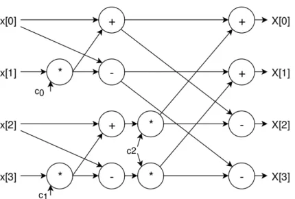
Data-driven architectures are a class of computer architectures where operations are triggered by the availability of data as operands, rather than a requirement for the results [17] as in a traditional von-Neumann architecture. Dataflow circuits are an implementation of a data-driven architecture. They consist of hardware components for various operations which are connected to reflect the natural flow of data in the algorithm. An example of a dataflow circuit is shown in Fig. 1.1.

High-level Synthesis (HLS) is the compilation of algorithms expressed in high-level languages such as C/C++/SystemC or functional languages to digital hardware expressed in a Register-Transfer Level (RTL) language such as Verilog or VHDL. The output, a netlist, can be used by a logic synthesis tool to synthesize a gate-level dataflow circuit that implements the algorithm. This gate-level description may be used by VLSI tools to fabricate ASICs or to program an FPGA.

1.2 Scheduling and Elastic Circuits

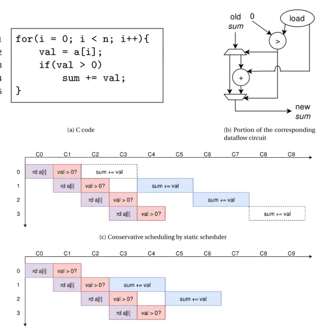
Scheduling in a dataflow circuit is the activation of the hardware elements of the circuit to per-form their function. Most existing HLS frameworks use static scheduling where the schedule is set at compile time and a central scheduling unit may be responsible for these activations. When control and/or data dependencies are indeterminable at compile time, static schedulers follow conservative schedules based on worst-case assumptions. This is demonstrated in Fig. 1.2, where the static scheduler must assume that the summation operation from the previous iteration might execute, and must delay the current operation accordingly. On the other hand, a dynamic scheduler can execute the current summation earlier, if the previous value is not positive.

corre-Figure 1.1 – Dataflow circuit for computing the Discrete Fourier Transform of a 4-wide array

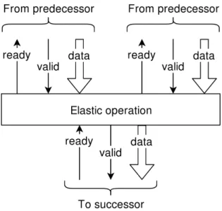
sponds to a node in a dataflow-graph. Nodes are activated dynamically when they are ready (to perform their operation) and their operands are available. Each component is augmented withreadyandvalidsignals to its predecessor and successor nodes, which forms a hand-shake mechanism for regulating the flow of data through the circuit. An example elastic node with two predecessors and a single successor is shown in Fig. 1.3. When data passes from one element to the next, a token is said to have passed between them. Unlike statically-scheduled circuits, there is no central scheduling unit activating elements according to some pre-determined schedule. Josipovic et al. [11] propose an algorithm for generating elastic circuits from C code.

1.3 LLVM

The LLVM Project is a research initiative that was started at the University of Illinois to de-sign a comprehensive, modular compiler framework [12, 13]. It includes compiler frontends for a variety of programming languages including C/C++/Objective-C which compile code to LLVM-IR, an intermediate representation in Static Single Assignment (SSA) form with a simple, language-independent type-system that can cleanly represent code in high-level languages [14]. External projects have extended frontend support to other high-level lan-guages such as Python, Java and Haskell. LLVM-IR is the basis of a number of analysis and transformation passes which respectively aim to generate insights about the code and to optimize it. Several commonly-used passes are included with the project, while most external projects implement passes of their own. LLVM also provides backends for generating static and just-in-time (JIT) code for popular existing architectures such as ARM, x86, and MIPS as well as research architectures such as RISC-V.

1.3. LLVM 1

for(i = 0; i < n; i++){

val = a[i];

if(val > 0)

sum += val;

}

(a) C code (b) Portion of the corresponding dataflow circuit

(c) Conservative scheduling by static scheduler

(d) Possible optimal schedule by dynamic scheduler

Figure 1.2 – Example code to compute the sum of all positive elements in an array. Fig. 1.2b shows a portion of the corresponding dataflow circuit. A static schedule may produce the schedule shown in Fig. 1.2c. In contrast, a dynamic scheduler may produce the optimal schedule shown in Fig. 1.2d.

Figure 1.3 – A node in an elastic circuit withreadyandvalidsignals which regulate the flow of tokens

1.3.1 Pass Infrastructure

LLVM includes a number of analysis and transformation passes which operate on LLVM-IR [15]. These are the basis for LLVM’s multi-stage optimization paradigm. Analysis passes generate information about the code which the transformation passes may exploit to generate optimized code. Commonly used analysis passes include:

• Alias Analysis - which checks whether or not two pointers may alias i.e. reference the same location. It is implemented by various modules which provide information at vari-ous levels of analysis. For example, BasicAA distinguishes between distinct global, stack and heap allocated variables. It also disambiguates different members of a struct, indices into arrays with statically different subscripts. SteensAA, implements a variation of the Steengaard’s Points-To analysis algorithm and is capable of providing inter-procedural alias analysis.

• Loop Information - which generates information about loops such their depth and contained basic blocks. Basic blocks within loops have an associated level (≥1) where the outermost loop is at level 1 and each subsequent nesting raises the level by 1. • Dominator/Post-Dominator Tree - which computes the dominator/post dominator

tree1by analyzing the control-flow graph (CFG).

• Region Information - which generates a list of valid regions2in the CFG. 1_{https://en.wikipedia.org/wiki/Dominator_(graph_theory)}

2_{In LLVM-IR, a region is defined by a single-entry header and a single-exit footer basic blocks. It is a set all basic} blocks which are dominated by the header and post-dominated by the footer, excluding the footer.

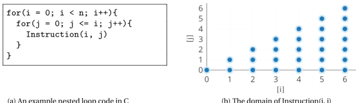
1.4. Integer Polyhedra 1 for(i = 0; i < n; i++){ 2 for(j = 0; j <= i; j++){ 3 Instruction(i, j) 4 } 5 }

(a) An example nested loop code in C (b) The domain of Instruction(i, j)

Figure 1.4 – The domain for an instruction inside a nested-loop in C is shown to form a polygon in 2-dimensional integer-space

1.4 Integer Polyhedra

An integer polyhedronP is defined as a set ofmdimensional vectors of the formP={x∈

Zm

|Ax≤b} for some matrixA∈Zm×nand some vectorb∈Zn. An integer polyhedron is often an apt descriptor for the domains of induction variables3for loops in a high-level language. As an example, the induction variables in the code from Fig. 1.4a are bound by the constraints 0≤j≤i<n. The execution domain for the instruction is described by the set shown below.

n [i,j] :³ 10 −01 −1 1 ´ ¡i j ¢ ≤ ³_n−1 0 0 ´o

1.4.1 Integer Set Library

The Integer Set Libraryislis a C library for creating and manipulating sets and relations of integer tuples bounded by affine constraints [18]. Among others,isldefines data structures representing the following types of objects4:

• Basic Integer Set • Set

• Basic Map • Map

3_{An induction variable is a variable that gets increased or decreased by a fixed amount on every iteration of} a loop. Without loss of generality, this thesis assumes that induction variables start at 0 and increase by 1 every iteration. Ref. Wikipedia

1 for(i = 0; i < n; i++){ 2 if(i % 2 == 0){ 3 from = i; 4 to = n - 1 - i; 5 a[to] = a[from]; 6 } 7 }

(a) (b) The array, before and after running the code. Arrows show the copying of data.

Figure 1.5 – Code to generate a palindromic array from the elements at even position of an array

Definition 1. Anislbasic set is a function S:Zn→2Zd:s7→S(s), where S(s)=©x∈Zd|∃z∈Ze:Ax+B s+D z+c≥0ª

with A∈Zm×d,B∈Zm×n,D∈Zm×e,c∈Zm.

In the definition,mis the number of constraints on the set,dis the number of set dimensions, nis the number of parameters andeis the number of existentially qualified variables. An example of a basic set is [n]→{i|∃e: 0≤i <n,i =2e}. This basic set can be used to represent the execution domains for the load and store instructions from the loop in Fig. 1.5a. The induction variableiis used to parse through the even positions in an array of sizen. The same set can be represented as:

[n]→ ½ [i] :³ 1 −1 1 −1 ´ ¡ i¢₊ ³0 1 0 0 ´ ¡ n¢₊ ³ 0 0 −2 2 ´ ¡ e¢₊ ³0 −1 0 0 ´ ≥0 ¾

where the constraints 0≤i<n,i=2eare re-arranged to get: • i≥0 and

• n−1−i≥0 • i−2e≥0 • −(i−2e)≥0

1.4. Integer Polyhedra • d=1 • m=4 • n=1 • e=1 • A=³ 1 −1 1 −1 ´ • B=³ 0 1 0 0 ´ • D=³ 0 0 −2 2 ´ • c=³ 0 −1 0 0 ´

Anislset is a union of a finite number ofislbasic sets, each of which have the same number of set and parameter dimensions.

Definition 2. Anislbasic map is a function M:Z→2Zd1×Zd2_{:s7→M(s)where}

M(s)=©

x1→x2∈Zd1×Zd2|∃z∈Ze:A1x1+A2x2+B s+D z+c≥0ª

with A1∈Zm×d1,A2∈Zm×d2,B∈Zm×n,D∈Zm×e,c∈Zm

In the definition,d1is the number of input dimensions,d2is the number of output dimensions,

mis the number of constraints on the set,nis the number of parameters andeis the number of existentially qualified variables.

An example of a basic map is [n]→{i→o:o=n−1−i}. This basic map can be used to represent the access relation for the store instruction in the loop from Fig. 1.5a. The location at indexn−1−iis accessed in theit hiteration. The same map can be represented as

[n]→n[i]→[o] :¡₋1₁¢¡i¢₊¡₋1₁¢¡o¢₊¡−₁1¢¡n¢¡1

−1 ¢

≥0o where the constrainto=n−1−iis expressed as:

• i+o−n+1≥0 and • −(i+o−n+1)≥0

To express the same basic map as per definition 2, • d1=1 • d2=1 • m=2 • n=1 • e=0 • A1=¡₋11 ¢ • A2=¡₋11 ¢ • B=¡−11 ¢ • D=¡¢ • c=¡₋11 ¢

Anislmap is a finite union of basic maps, each of which have the same number of input, output and parameter dimensions.

For the purpose of readability, constraints onislsets and maps will be written as a list for the rest of the document. Syntactic sugar (e.g. ’i mod 2 = 0’) will be used where possible.

1.5 Polly

Polly is a framework based on LLVM which uses polyhedral analysis to optimize loops within programs for data locality and parallelism [7]. Implemented as a series of LLVM passes, Polly includes separate modules for preparing code for Polly (canonicalization), detecting SCoPs and creating polyhedral descriptions for memory accesses, optimizing them and re-generating the IR.

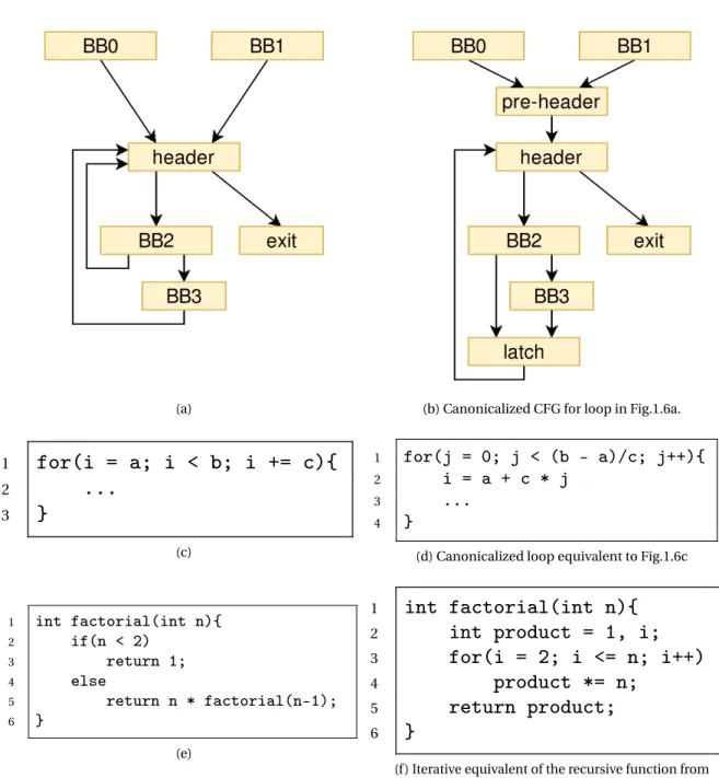
Polly performs the following loop canonicalization passes:

• Loop Simplification: This pass ensures that each loop has a pre-header from which there is a single entry-edge to the loop header. It also ensures that the loop has a single latch edge5like in Fig.1.6b.

• Induction variable canonicalization: This modifies each loop to have a single induction variable counting from zero with steps of one, like in Fig. 1.6d.

• Tail call elimination: This pass transforms tail-recursive functions into their iterative form. This enables Polly to analyze and optimize loops written in functional program-ming languages or with functional paradigms in mind like in Fig. 1.6f.

1.5.1 Static Control Parts

Static Control Parts are regions of a program in which all control flow decisions and memory accesses are known at compile time and hence, may be statically scheduled by a control unit. SCoPs must be side-effect free [6] and contained loops must have affine expressions in induction variables and parameters for:

• Loop bounds.

• Flow control conditions. • Memory access relations.

Examples of loops which are SCoPs can be found in Fig. 1.5a and Fig. 1.8 while loops which violate one or more of these conditions are shown in Fig. 1.7.

1.5.2 ScopInfo Pass

The pass ScopInfo implemented by Polly detects SCoP regions and creates polyhedral descrip-tions for memory accesses in them. Grosser [7] defines a SCoP in LLVM-IR and describes the

1.5. Polly

(a) (b) Canonicalized CFG for loop in Fig.1.6a.

1

for(i = a; i < b; i += c){

...

}

(d) Canonicalized loop equivalent to Fig.1.6c

1 int factorial(int n){ 2 if(n < 2) 3 return 1; 4 else 5 return n * factorial(n-1); 6 } (e) 1

int factorial(int n){

int product = 1, i;

for(i = 2; i <= n; i++)

product *= n;

return product;

}

(f ) Iterative equivalent of the recursive function from Fig.1.6e

1

for(i = 0; i*i < n; i++){

lock(i);

3

a[i] = i;

unlock();

5

}

(a) Loop has a non-affine upper-bound and function calls with side-effects (modifies a lock variable)

1

while(low < high){

2

mid = (low + high)/2;

if(a[mid] == n)

...

else if(a[mid] < n)

low = mid + 1;

else if(a[mid] > n)

high = mid;

}

(b) Loop has data-dependent control decisions and loop bound

Figure 1.7 – Two non-SCoP loop regions. The algorithm in Fig. 1.7a acquires a lock before writing to the array at indexi. Fig. 1.7b shows an implementation of the binary search algorithm.

SCoP-detection algorithm. The ScopInfo pass analyzes the LLVM-IR representation allowing detection of regions that are semantically a SCoP, but are not expressed as such. Examples may be seen in Fig. 1.8.

For every valid region, ScopInfo creates a Scop object containing ScopStmt objects corre-sponding to each contained basic block. A description is generated for each memory access (load/store) in a MemoryAccess object comprising a domain, a schedule, a base and an access relation map.

• The base for a MemoryAccess is a pointer to the base of the array accessed by the instruction.

• For an instructionI nested insidemloops, the domainD for a MemoryAccess is the set of vectorsvi nd={v1, . . .vm} of the values of induction variables for whichIwill be

executed. Eachvirefers to the value of the induction variable for the loop at leveli. Therefore,v1is the value of the induction variable for the outermost loop andvm is the

value of the induction variable for the innermost loop. Polly describes the domain for an instruction in anislset object. Values from outside the outermost loop which are used in the SCoP are specified as parameters.

• The access relationship for a MemoryAccess is a function that maps a vector ofm induc-tion variables to a vector ofnindices into then-dimensional base array. Polly represents the access relationship as anislmap object. Values from outside the outermost loop which are used in the SCoP are specified as parameters.

1.6. Elastic Compiler 1 i = 0; 2 3 do { 4 int a = 3 * i; 5 int b = n/2 + i + 5 * a; 6 7 arr[b] = i; 8 i += c; 9 } while (i < n);

(a) Using a complicated index expression

1 for(i = 0; i == 0 || i < n; i += c){ 2 arr[n/2 + 16 * i] = i;

3 }

(b) Equivalent code in canonical form

1

int *iter = arr;

2

int *end = &arr[n];

3

int count = 0;

4

5

while(iter != end) {

6

*iter++ = count++;

7

}

(c) Using pointer arithmetic to parse an array

1

for(i = 0; i < n; i++)

arr[i] = i;

(d) Equivalent code in canonical form Figure 1.8 – Two valid SCoP regions and their canonicalized counterparts

• The schedule is a vector which allows for partial ordering on the set of memory instruc-tions within a SCoP. This information is used by Polly for analyzing memory dependen-cies and parallelizing loops.

1.6 Elastic Compiler

The Elastic Compiler (EC) under development at EPFL implements the HLS strategy as pro-posed in Josipovic et al. [11] and is based on the LLVM compiler infrastructure. Starting from the intermediate representation generated by an LLVM frontend (e.g. Clang) and its corresponding CFG, the Elastic Compiler generates a VHDL netlist for a dynamically sched-uled circuit. The circuit comprises elements implementing specific basic operations (e.g. arithmetic, branch, select) similar to those in traditional dataflow circuits, but augmented with elastic control signals connecting each element to its predecessors and successors in order to achieve latency-insensitive scheduling. It also includes other elastic components such as elastic buffers, elastic FIFOs, eager and lazy forks and joins. These are described in detail in previous work [4, 9]. Connections to arrays of random-access-memory (RAM) are made through read and write ports that connect to an arbitrator or a load-store-queue. The connection to memory is the focus of this work and is described in more detail in chapter 2. Elastic sub-circuits are first generated for each basic block by literally translating the dataflow

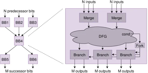
Figure 1.9 – The template for generating elastic basic blocks

graph by replacing operators with their corresponding functional units, connecting compo-nents to their predecessors and successors and introducing forks wherever the output of a component has more than one successor (at least one of which is within the same basic block). Control nodes resembling a data-less variable are added for each block. These sub-circuits are then augmented with branch nodes for each live value leaving a basic block and merge nodes for each value entering it. Finally, the sub-circuits are stitched together. For each basic block edge in the CFG, the branch node from the predecessor for each live value is connected to the corresponding merge node in the successor. This is illustrated in Fig. 1.9 reproduced from Jospovic et al. [11]. Other added components include FIFOs to decouple fast paths from slower ones, and buffers to break combinatorial loops or critical edges.

2

Memory Dependencies in Elastic

Cir-cuits

Nodes in an elastic circuit are dynamically scheduled when their operands are available. As a result, the temporal ordering between the activations of any arbitrary pair of nodes in the circuit is unclear at compile time and memory accesses are inherently out-of-order. The flow of tokens through the circuit provides us with the only mechanism for temporally ordering the activations of pairs of nodes where one depends on the other for receiving a token, and hence being activated. Nodes corresponding to memory instructions (load/store) may have read-after-write (RAW) and write-after-write (WAW) dependencies. Being out-of-order, these nodes might need a load-store-queue (LSQ) to dynamically resolve memory dependencies and correctly order dependent accesses.

Load-store queues are structures that allow memory operations to be issued to memory out-of-order by checking addresses with all previous operations. For example, a load may be issued to the RAM as soon as all previous store addresses are available to the LSQ and it verifies that none of them write to the same address as the load. For this purpose, it uses Content-Addressable Memory (CAM) which incorporates comparison circuitry with every address storage cell. Since every address must be compared with all previous addresses, the hardware and energy costs of an LSQ increase super-linearly with its size, i.e. the number of outstanding memory operations it can handle.

An LSQ must be sized to handle the latency between a load entering the queue and addresses for all previous stores becoming available. To store all addresses that arrive in this period, the size of its queues must increase with the number of read and write ports. As a result, it is desirable to only connect memory components to the relevant LSQ if there might be RAW/WAW dependencies at runtime.

2.1 Elastic compiler: Memory access

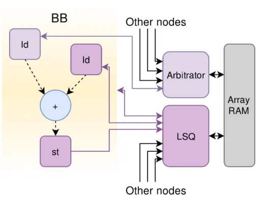
Memory components in the circuits generated by the Elastic Compiler (EC) are connected to arrays of dual-ported random-access memory (RAM). Each RAM corresponds to an array in

Figure 2.1 – Elastic memory components may be connected to the memory via an arbitrator or an LSQ. The LSQ also has a control connection to the basic blocks from which it has read/write connections

the C-representation of the algorithm. The hardware node for a memory element might be a simple port which connects to an arbitrator that uses one of the RAM ports or a connection to a LSQ that uses the other RAM port.

EC implements LSQs as described in Josipovic et al. [10]. Elastic components corresponding to memory instructions are connected to the relevant LSQ via elastic interfaces which include separate elastic signals for the data and address. An example connection is shown in Fig 2.2. When control reaches a basic block, slots corresponding to the loads and stores in the block are allocated in the LSQ prior to any of those components being activated. In the existing EC compiler, memory nodes need to be manually connected to the memory subsystem. Further, they are all conservatively attached to the LSQ.

In this work, we extend EC by automating and optimizing the assignment of memory nodes to LSQs. We describe the insights which allow the compiler to make the decision to connect to memory via a simple port to the arbitrator instead of the LSQ. Further, it describes the implementation of memory disambiguation passes based on these insights in EC which allows it to automate the process of connecting the elastic circuit to memory. An example of a portion of a possible circuit generated by the final compiler is shown in Fig. 2.1. In this example, the load node connected to the arbitrator must have been proved to be independent of all other nodes accessing the same RAM.

2.2. Architecture

Figure 2.2 – Generated LSQs have connections to elastic read/write ports and to their basic blocks. Yellow blocks represent basic blocks.

In the augmented EC infrastructure, the MemElemPass analysis pass generates a MemElem-Info object containing information used while generating the hardware components for accessing memory. For each node corresponding to a memory instruction, we can query whether it requires an LSQ connection or a basic memory port, and which RAM it needs to access, in order to connect it correctly. Finally, MemElemInfo tracks the necessary control connections between basic blocks and LSQs for slot allocation [10].

2.2 Architecture

The architecture of the memory dependence analysis infrastructure is shown in Fig. 2.3. Nodes indicate analyses while arrows from Node A to Node B indicates that analysis A depends on results produced by analysis B.

Token dependence is defined in Chapter 3 and relates the flow of tokens between pairs of circuit components within a loop. The TokenDependenceInfo class presents the query interface for this analysis.

Figure 2.3 – Analysis passes for analyzing memory dependencies between instructions. Arrows indicate dependences between passes.

uses polyhedral information from the ScopInfo wrapper pass to create sets of indices accessed by each instruction and then checks for overlapping sets to detect possible dependencies. It also uses token dependence information from the TokenDependence analysis to temporally relate the activations of memory operations to further rule out dependencies.

MemElemInfo provides the high-level abstraction that the compiler can use to assign hardware components to memory operations. It uses information from IndexAnalysis and AliasAnalysis passes to detect pairs of instructions with memory dependencies and thereby create sets of instructions to be assigned to every LSQ. This pass is described in Chapter 5.

3

TokenDependenceInfo

The TokenDependenceInfo class tries to determine if there is a token dependence or reverse dependence, as defined below, between a pair of instructions by examining the LLVM-IR generated by the compiler frontend.

We define two types of token dependence to describe the flow of tokens between a pair of nodes:

• Token Dependence

• Reverse Token Dependence

Definition 3. An instruction IB is dependent on IA(written as IA D

−→IB) w.r.t. a set Si nd of induction variables if every token arriving at the node corresponding to IB has passed through the node for IA without passing though basic block edges that would increment any of the induction variables in Si nd.

Definition 4. An instruction IA is reverse dependent on IB (written as IA−−→RD IB) w.r.t. a set Si nd of induction variables if every token arriving at the node corresponding to IAwill flow to the node for IBwithout passing through basic block edges that would increment any of the induction variables in Si nd.

In Fig. 3.1, we see a snippet of C code, its intermediate representation in LLVM and a portion of the elastic circuit generated as a result. From the LLVM code, we can find the following dependences, among others:

• I0 D −→I1 • I1 D −→I2 • I2−→D I3 • I3 D −→I4 • I3 D −→I5 • I3 D −→I8 • I3 D −→I9 • I6 D −→I8 • I7 D −→I8 • I8−→D I9

However, we can also determine that the instructionI6does not have a token dependence on

Also, there is no token dependence betweenI4andI5because there is no path between them

without incrementing the induction variablei.

The elastic circuit also has the following reverse dependencies, among others: • I3 RD −−→I8 • I3 RD −−→I9 • I4 RD −−→I6 • I4 RD −−→I8 • I4 RD −−→I9 • I5 RD −−→I7 • I5 RD −−→I8 • I5 RD −−→I9 • I6 RD −−→I8 • I6 RD −−→I9 • I7 RD −−→I8 • I7 RD −−→I9 • I8 RD −−→I9

In contrast, the instructionI4does not have a reverse dependence onI5since there is no path

from the basic-blockif.thentoif.elsewithout incrementing the induction variablei.I4also

does not have a reverse dependence onI7since there is a path in whichI7gets a token from

the node with the constant value 1.

3.1 Properties

1. If IA−→D IB,B BAdominates1B BB. 2. If IA

RD

−−→IB,B BB post-dominates2B BA.

3. Both dependence and reverse dependence are transitive, symmetric and non-reflexive.

4. If IA −→D IB w.r.t the set of common induction variablesSi nd, IA cannot be within a deeper loop body.

5. If IA−−→RD IB w.r.t the set of common induction variablesSi nd,IB cannot be within a deeper loop body.

6. If IA

D

−→IBor IA

RD

−−→IBw.r.t the set of common induction variablesSi nd, every execution ofIAfor iteration vector3vwill finish before any execution ofIBfor the same iteration vector.

7. If IA−→D IBor IA−−→RD IBw.r.t the set of common induction variablesSi nd, every execution ofIAfor iteration vectorvA≤v0will finish before any execution ofIBstarts for iteration vectorvB≥v0.

1_{In control-flow graphs, a basic blockB B}

Adominates anotherB BBif every path from the entry node toB BB

must pass throughB BA.

2_{In control-flow graphs, a basic blockB B}

Bpost-dominates another basic blockB BAif every path fromB BAto

the exit node must pass throughB BB.

3_{The vector of the values of induction variables in use at a certain time forms the iteration vector. Comparisons} of iteration vectors are done lexicographically.

3.1. Properties

1 for(i = 0; i < n; i++) {

2 int val = a[i];

3 if(cond){ 4 op0 = val; 5 op1 = 1; 6 } else { 7 op0 = -1; 8 op1 = val; 9 }

10 a[i] = op0 * op1;

11 }

(a) C code (b) Portion of the elastic circuit

1 for.head:

2 %i = phi i32 [0, %entry], [%i.inc, %if.end] ...(I0) 3 %cmp = icmp slt i32 %i, %n

4 br i1 %cmp, label %if.entry, label %final 5 if.entry:

6 %idx = sext i32 %i to i64 ...(I1)

7 %ptr = getelementptr inbounds i32, i32* %vla, i64 %idx ...(I2) 8 %val = load i32, i32* %ptr, align 4 ...(I3) 9 br i1 %cond, label %if.then, label %if.else

10 if.then:

11 %0 = %val ...(I4)

12 if.else:

13 %1 = %val ...(I5)

14 if.end:

15 %op0 = phi i32 [%0, %if.then], [-1, %if.else] ...(I6) 16 %op1 = phi i32 [1, %if.then], [%1, %if.else] ...(I7)

17 %mul = mul nsw i32 %op0, %op1 ...(I8)

18 store i32 %mul, i32* %ptr, align 4 ...(I9) 19 %i.inc = add nsw i32 %i, 1

20 br label %for.head

(c) LLVM code

3.2 Proofs of properties

D

−→IB, butB BAdoes not dominateB BB, the token may flow toIBalong a path that does not pass throughB BA.IBwill execute with a token that has not passed throughIA. This violates the definition of token dependence.

2. If IA

RD

−−→IB, butB BBdoes not post-dominateB BA, the token may flow fromIAalong a path that does not pass throughB BB. IAwill execute on a token that shall not pass throughIB. This violates the definition of token reverse dependence.

3. The proof is trivial and omitted.

4. IfIAis in a deeper inner-loop,B BAdoes not dominateB BBsince the inner-loop might never be entered. This result follows from property 1.

5. IfIB is in a deeper inner-loop,B BB does not post-dominateB BAsince the inner-loop might never be entered. This result follows from property 2.

6. Given IA

D

−→ IB, every token reaching IA must have the same iteration vectorv for common induction variables.IBmight be within a deeper loop and execute multiple times, butIAmight not by property 4. By the properties of elastic circuits, the deeper loop will be entered after the token flows throughIA. Similarly, given IA−−→RD IB,IA might be in a deeper loop, butIB might not by property 5. In an elastic circuit, the deeper loop will complete before the token flows toIB. If neither are in deeper loops, the token flow is obvious. In all cases, the property holds.

7. From property 6, the execution ofIBfor iteration vectorv0is strictly after the execution

ofIAfor the same iteration vector. Elastic circuits have the property that each node processes all of its tokens in-order. Thus, the node forIAwill process tokens forvA<v0

before that forv0followed byIB processing the token forv0 and, finally, tokens for

vB>v0.

3.3 Finding dependence relations

Let us consider instructionsIA(in basic blockB BA) andIB (in basic blockB BB). LetSi nd be the set of induction variables corresponding to loops common to both instructions.

Definition 5. A valid path P w.r.t. a set of induction variables Si nd is a vector of basic blocks [B B1, . . .B Bn]such that

• ∀i∈{1, ...n−1}B Bito B Bi+1is an edge in the CFG.

• B Bnis the latch block4for the innermost loop whose induction variable is in Si nd or • B B1is the header block for the innermost loop whose induction variable is in Si nd

3.3. Finding dependence relations

The definition above assumes a canonicalized CFG where each loop has unique header and latch blocks.

For determining token dependence/reverse-dependence relations, we need to track the flow of tokens along every path that the program may take through the CFG. If we want to check if IA−→D IB holds, we need to find out the various valid paths to the basic block containingIB and confirm that along each of these paths,IB directly or indirectly uses the value produced byIA. Conversely, to explore whether IA

RD

−−→IB, we need to find the various valid paths from the basic block containingIAand confirm that along each of these paths, the value produced byIAis used byIB.

TheK−setsas defined below track those instructions that produce values on which an instruc-tionIB directly or indirectly depend. Each sequence ofK−sets(K0,K1, ...,Kn) is defined for

a pathP=[B B1, . . .B Bn].Knis defined to contain onlyIB. IfB Bi+1toB Bnare the finaln−i

blocks inP,Kifori<ncontains those instructions in these basic-blocks on whichIBdepends. As we work backwards along a path, moving fromB Bi₊1toB Bi, we add those instructions

inB Bito the setKi−1if it produces a value used inKior itself. IfB BAappears at a position

i=iAin the pathP,IB is directly or indirectly dependent on the value produced byIAiffKiA−1

containsIA. Therefore, to check for token dependence, this condition needs to be checked for each valid path.

Definition 6. For each path P=[B B1, . . .B Bn],∀i<n we define the set Ki corresponding to the

basic block B Bi₊1in the path as

Ki=Ki+1

∪©v|∃w:w∈B Bi,w∈Ki₊1,v∈operands(w)ª

∪©v|∃w:w∈B Bi,w ∈ Ki,v∈operands(w)ª

For phi instructions, only the operand corresponding to the previous basic block B Bi−1 is

considered. The set Knis specially defined.

Similarly, theM−setsas defined below track those instructions that use the value produced byIAdirectly or indirectly. Each sequence ofM−sets(M0,M1, ...,Mn) is defined for a path P=[B B1, . . .B Bn]. M0is defined to contain onlyIA. IfB B0toB Bi are the firstiblocks inP,

Mifori>0 contains those instructions in these basic-blocks which depend onIA. As we work our way along a path, moving fromB BitoB Bi+1, we add those instructions inB Bi+1to the

setMi+1which use values produced by instructions inMior itself. IfB BB occurs at position

i=iB in the pathP,IB is directly or indirectly dependent on the value produced byIAiffMiB

containsIB. Therefore, to check for reverse token dependence, this condition needs to be checked for each valid path.

Definition 7. For each path P=[B B1, . . .B Bn],∀i>0we define the set Micorresponding to the

basic block B Bi in the path as Mi=Mi₋1 ∪© v|∃w:v∈B Bi,w∈Mi−1,w∈operands(v)ª ∪© v|∃w:v∈B Bi,w∈Mi,w∈operands(v)ª

For phi instructions, only the operand corresponding to the previous basic block B Bi−1 is

considered. The set M0is specially defined.

3.3.1 Dependence

ForKn={IB}, IA−→D IB if∀valid pathsPending inB BB, • P containsB BAat least once, and

• IfB BAfirst occurs at indexiinP,Ki₋1containsIA.

Examples

Consider the example code in Fig. 3.1. Let us see if I3−→D I9. The two valid paths ending in the

basic block forI9,if.end, areP0=[for.head,if.entry,if.then,if.end] andP1=[for.head,if.entry,

if.else,if.end]. The basic block containingI3isif.entry.

• ForP0, the K-sets are shown in Fig. 3.2a. ForK3the previous basic block isif.then, and

only operand %0 is considered forI6and the constant 1 forI7. It can be seen that the

basic blockif.entryoccurs at index 2 andI3∈K1. For this path,I3produces a value

indirectly used byI9.

• ForP1, the K-sets are shown in Fig. 3.2b. ForK3the previous basic block isif.else, and

only operand %1 is considered forI7and the constant−1 forI6. It can be seen that the

basic blockif.entryoccurs at index 2, andI3∈K1. For this path as well,I3produces a

value indirectly used byI9.

It can be seen that the conditions hold for both paths, implying I3 D

−→I9.

Now, let us see if I3 D

−→I6. The two valid paths are as in the previous example.

• ForP0, the K-sets are shown in Fig. 3.3a. ForK3, the previous basic block isif.thenand

only operand %0 is considered forI6. The conditions hold for this path. For this path,I3

3.3. Finding dependence relations

• K4={I9}

• K3={I9,I8,I7,I6,I4,I2}

• K2={I9,I8,I7,I6,I4,I3,I2}

• K1={I9,I8,I7,I6,I4,I3,I2,I1,I0}

(a) K-sets for pathP0

• K4={I9}

• K3={I9,I8,I7,I6,I5,I2}

• K2={I9,I8,I7,I6,I5,I3,I2}

• K1={I9,I8,I7,I6,I5,I3,I2,I1,I0}

(b) K-sets for pathP1 Figure 3.2 – K-sets for determining if I3

D −→I9in Fig. 3.1c • K4={I6} • K3={I6,I4} • K2={I6,I4,I3} • K1={I6,I4,I3,I2,I1,I0}

(a) K-sets for pathP0

• K4={I6}

• K3={I6}

• K2={I6}

• K1={I6}

(b) K-sets for pathP1 Figure 3.3 – K-sets for determining if I3

D

−→I6in Fig. 3.1c

• ForP1, the K-sets are shown in Fig. 3.3b. ForK3, the previous basic block isif.elseand

only the constant−1 is considered forI6. The basic blockif.entryoccurs once at index

2 andI3∉K1, so the conditions do not hold for this path. For this path,I3does not

produce a value used byI9.

The conditions do not hold for pathP1. Therefore, there is no dependence.

3.3.2 Reverse Dependence ForM0={IA}, IA

RD

−−→IBif∀valid pathsP starting inB BA, • P containsB BB at-least once

• IfB BBlast occurs at indexiinP,MicontainsIB.

Examples

Consider the example code in Fig. 3.1. Let us see if I3−−→RD I9. The two valid paths starting in

the basic block forI3,if.entry, areP0=[if.entry, if.then, if.end] andP1=[if.entry, if.else, if.end].

The basic block containingI9isif.end.

• ForP0, the M-sets are shown in Fig. 3.4a. It can be seen that the basic blockif.end

• M0={I3}

• M1={I3}

• M2={I3,I4}

• M3={I3,I4,I6,I8,I9}

(a) M-sets for pathP0

• M0={I3}

• M1={I3}

• M2={I3,I5}

• M3={I3,I5,I7,I8,I9}

(b) M-sets for pathP1 Figure 3.4 – M-sets for determining if I3

RD

−−→I9/I3 RD

−−→I6in Fig. 3.1c

• ForP1, the M-sets are shown in Fig. 3.4b. It can be seen that the basic blockif.end

appears at index 3, andI9∈M3. For this path as well,I3produces a value indirectly used

byI9.

Since the conditions hold for all paths, I3−−→RD I9.

Now, let us see if I3 RD

−−→I6. The two valid paths and their M-sets are as in the previous example.

We can see that the conditions hold on pathP0but not on pathP1(I6∉M3), implying that

4

IndexAnalysisInfo

IndexAnalysisInfo checks for memory dependences between memory accesses in a SCoP. Implemented as a LLVM FunctionPass (IndexAnalysisPass), this EC component analyzes the indices within an array accessed by load/store instructions to decide if the same location may be accessed by different instructions.

In the example from Fig. 4.1, the load instruction accesses the first half of the string, while the store accesses the second half of the string. In other words, the set of accessed indices by the load is {0, . . .bn/2c −1} while that for the store is {dn/2e, . . .n−1}. It can be seen that the above sets are disjoint, ruling out the possibility of a RAW dependency.

When a pair of instructions access memory locations in the same array, an analysis of accessed indices may reveal that they cannot access the same address. This is the insight behind IndexAnalysisInfo as a memory disambiguation pass.

It uses TokenDependenceInfo as described in chapter 3 to determine if pairs of instructions have token dependences or reverse token dependences. Either dependence can be used to temporally relate activations of memory nodes and thereby rule out certain memory depen-dencies. Consider an example where stores to an array at indices 1 to 5 precede loads to the same. The accesses are demonstrated in the example shown in Fig. 4.2. All the stores should complete before the loads. Without timing information, we cannot be sure that any of the stores actually happens before the load to the same address. Therefore, all the accesses might violate memory dependencies as shown in Fig. 4.2. With cycle information as shown in

1

int n = strlen(str);

2

for(i = 0; i < n/2; i++){

3

str[n-1-i] = str[i];

4

}

(a) Without timing information, we cannot know if the write actually precedes the read to the same index. In this example, every read may potentially violate RAW dependencies.

(b) With timing information, we can see that the last two reads definitely respect RAW dependencies.

Figure 4.2 – Violations of read-after-write (RAW) dependencies, indicated by arrows, between instructions accessing the arrayawhere the store programmatically precedes the load.

Fig. 4.2b, we can see that the accesses for indices 1 and 2 are properly ordered while those for indices 3, 4 and 5 might not be.

4.1 Information from Polly

The IndexAnalysisInfo pass requires precise information about the index within an array accessed by each memory instruction. For SCoPs, Polly is able to provide this information from its ScopInfoWrapperPass. This pass generatesScopobjects containing domain sets(Dom), bases(B ase) and access relations(AR) for each memory access instruction in the SCoP. For the example in Fig. 4.1, Polly gives us the following information:

• For the load:

– Domain: [n]→©

[i] : 0≤i<floor(n/2)ª

– Base: Arraystr

– Access relation: [n]→©[i]→[o] :o=iª

• For the store:

– Domain: [n]→©[i] : 0≤i<floor(n/2)ª

– Base: Arraystr

– Access relation: [n]→©

4.2. Base algorithm

4.2 Base algorithm

IndexAnalysisInfo analyzes pairs (IA,IB) of instructions within a SCoP. For RAW/WAW depen-dences to exist between the statements:

• at least one of them must write to memory,

• both instructions must access the same array which is stored in a unique RAM structure in the circuit, and

• there must exist vectors of induction variablesvA,vB and a vector of array indicesi d x such thatvA∈DomA,vB∈DomB, (vA→i d x)∈ARAand (vB→i d x)∈ARB.

For pairs of instructions that satisfy the first two conditions, IndexAnalysisInfo creates the sets {o|∃i:i∈Dom,i→o∈AR} for both. If these sets are disjoint, there are no memory dependen-cies between them.

4.3 Exploiting Token Dependence

In section 4.2, we discussed the algorithm allowing us to statically analyze memory accesses for memory dependencies within a SCoP. However, in certain cases, the properties of token flow in elastic circuits as discussed in Chapter 3 allow us to put restrictions between the iteration vectors being processed by a pair memory nodes. These additional restrictions might allow us to rule out certain dependencies as illustrated in Fig. 4.2. When we can statically determine that the read and store to an address must happen in the same order in an elastic circuit as in the LLVM code, we do not need an LSQ to order them.

If IA is a load instruction,IB is a store instruction currently executing iteration vectorvB andSi nd is the set of induction variables for loops common to both instructions, property 7 from section 3.1 assures us that every execution ofIAfor iteration vectorsvA<vBwill have completed if IA

D

−→IBor IA

RD

−−→IBw.r.tSi nd. We only need to check if the store for iteration vectorvB and the load for lexicographically larger iteration vectors can access the same array index. Since we cannot determine the temporal ordering between them, RAW dependency violations are possible and we need to connect them to a LSQ.

Consider the example in Fig. 4.3 in which the elements of an array are shifted forward by one position. Based on SCoP analysis, we know that the set of indices accessed by the load is {1, 2, ...,n−1} while the set of indices accessed by the store is {0, 1, ...,n−2}. Since the same indices are accessed by both instructions, RAW dependencies between the load and the store seem possible. However, token dependence implies that, in an elastic circuit, the store to any index must happen after the load to the same index, as explained hereon. When the store is storing to the indexiBin iterationi=iB, the load for all iterationsi≤iB must have finished. Possible read indices in the future are to indexiA+1 for iterationsiA>iB. The store toiBcannot be read in the future which proves that RAW dependences are practically impossible in this case.

1

for(i = 0; i < n - 1; i ++)

2

arr[i] = arr[i + 1];

Figure 4.3 – Example of a loop with intersecting read and write sets. Temporally ordering the operations by token dependence shows the lack of RAW dependencies.

4.3.1 Algorithm for dependent instructions

SupposeIAis a load instruction andIB is a store instruction such that IA−→D IBor IA−−→RD IB andSi nd is the set of induction variables for loops common to both instructions. For an iteration vectorv, letcommon(v) be the vector of values fromvcorresponding to members ofSi nd.

Definition 8. For a load instruction, theFuture load setis defined as:

       i→o|∃il d,il d0 : il d∈DomA,il d →o∈ARA, common(i_{l d}0 )<common(il d), i=common(i_{l d}0 )       

Definition 9. For a store instruction, theStore setis defined as:

(

i→o|∃ist:ist∈DomB,ist →o∈ARB, i=common(ist)

)

Suppose (i0→o0) is an element of both sets. By membership in the store set, there exists a

iterationist s.t. common(ist)=i0that accesseso0. By membership in the future load set,

there exists a later iterationil dfor which the load instruction accesses the array indexo0and

common(ist)<common(il d). A RAW dependence exists and since token flow cannot order these accesses, incorrect execution is possible in the absence of an LSQ.

Congruently, suppose there is a RAW dependency between the iteration il d of the load and the iterationist of the store, both of which access the same indexo0. It must be that

il d∈DomA, (il d→o0)∈ARA,ist∈DomB, (ist→o0)∈ARB. Token dependence implies that

common(ist)<common(il d). Therefore, (ist→o0) will be a member of both sets and the

intersection of the sets cannot be empty.

Let us follow along with the example code from Fig. 4.4 whereais a 3×3 array of integers. There is a reverse dependency from the load to the store.

• For the load

– Domain: [] → ©

[0, 0], [0, 1], [0, 2], [1, 0], [1, 1], [1, 2]ª

– Access Relation: [] → ©

4.3. Exploiting Token Dependence 1 for(i = 0; i < 2; i++) { 2 sum = 0; 3 for(j = 0; j < 3; j++) 4 sum += a[i][j]; 5 a[i + 1][0] = sum; 6 }

(a) Example code for adding rows of an array, storing the sum in the first space of the next row.

(b) Temporal ordering between memory accesses. Solid links indicate known temporal ordering due to token flow. Dotted links indicate unknown temporal ordering

Figure 4.4 – Illustrative example of code with token reverse dependence and showing temporal ordering relations

– Future Load Set:©

[0]→[1, 0], [0]→[1, 1], [0]→[1, 2]ª

• For the store

– Domain: [] → ©[0], [1]ª

– Access Relation: [] → ©

[i]→[i+1, 0]ª

– Store Set:©

[0]→[1, 0], [1]→[2, 0]ª

The timing relations due to token flow can be seen in Fig. 4.4b. The timing between the load for iteration [1, 0] and the store for iteration [0], both of which access the index [1, 0] in the array, cannot be determined. Hence, these instructions have a RAW dependency which may be violated if they use simple memory ports. As expected, the store and future load sets are non-disjoint.

5

MemElemInfo

MemElemInfo is a LLVM FunctionPass used by EC to make decisions while generating hard-ware components for nodes which access memory.

For loops, it uses IndexAnalysisInfo and AliasAnalysis to decide whether pairs of instructions may have memory dependencies. It is designed to be extensible i.e. to be able to consider more sub-analyses that can rule out dependencies for other special cases. Currently, it uses the dependency decision for IndexAnalysisInfo for a pair of instructions from the same SCoP. For all other pairs, it uses aliasing information.

After it generates a comprehensive list of such pairs, it creates sets of instructions accessing the same array base which require a LSQ.

The known shortcomings of the MemElemInfo analysis are:

• Since non-loop instructions do not practically affect the depth of the load-store-queue, all memory accesses for these instructions are assigned to a LSQ. However, we could use ports if token flow serializes these accesses.

• To limit the scope of other instructions with which an instruction may alias, MemElem-Info assumes serialization of top-level loops. This may lead to fewer components being connected to LSQs at the cost of increased execution time if the loops could significantly overlap at runtime. This presents a trade-off in the design space between performance and hardware/power costs.

6

Results

In this section, we show examples of code for which we have used the Elastic Compiler to generate VHDL circuits. We focus on three example kernels that demonstrate the utility of our insights and uses the passes discussed earlier to optimize the connections to LSQs required. For all examples, we use Clang as a frontend to compile the C-code to LLVM-IR without any optimization (-o0option). Next, they are run though some standard LLVM optimization passes to propagate constants (constprop), use registers instead of stack memory to pass values through the circuit (mem2reg), eliminate dead instructions (die) and simplify the CFG to remove trivial branches (simplifycfg). Finally, we use the EC to generate netlists in VHDL. We use this netlist to find the number of load/store ports used and their connections to LSQs, and to evaluate the cost of connecting to memory.

6.1 Methodology

We shall demonstrate the utility of each of our insights towards optimizing the generated circuit’s interface to memory, specifically the size of the LSQs, by running the Elastic Compiler on three code kernels. Each of these kernels demonstrates the utility of a separate part of the analysis architecture.

As discussed earlier, the size of the queues of an LSQ are directly related to the number of read and write ports connected to it. We currently have an implementation that automates the process of compilation upto generating the required VHDL netlist. However, we would also need to place and route our designs onto an FPGA using a tool such as Vivado to be able to accurately measure the power and resource requirements for the LSQ. As an equivalent, but approximate metric, we shall estimate the cost of an LSQ as the square of the sum of number of connected read and write ports.

For each code kernel, we shall compare the following cases:

• All memory components are connected to a single LSQ. We designate this as the base case.

• We use AliasAnalysis to distinguish accesses to different arrays, and use different queues for each. We refer to this case as AA.

• We use basic IndexAnalysis without TokenDependenceInfo to analyse accesses within an array. We shall refer to this case as IA.

• We use IndexAnalysis with ordering information from TokenDependenceInfo. We refer to this case as IA+TD.

Each case incorporates and improves upon the results of the previous case. Our implementa-tion in the Elastic Compiler corresponds to the final case listed above (i.e.IA+TD).

6.2 Test Cases

Here, we describe the test cases and the number of ports to LSQs at each step of the analysis. The final costs are summarized in Table 6.1. We can see that in these examples, our analysis results in LSQs that cost between 75% and 93% lesser than the base case.

6.2.1 Histogram kernel

The first kernel we analyze is shown in Fig. 6.1. The algorithm calculates an histogram with associated weights for every element. It is assumed that the elements of the feature vector lie in the [0,n) range. As can be seen, there are three load operations and a single store. AliasAnalysis allows us to determine that the loads to thefeatureandweightarrays do not need connections to LSQs. Only thehistarray requires an LSQ with one read and one write port. As the loop is not a Static Control Part, IndexAnalysis analysis is not possible.

Kernel Number of Number of Base Case AA IA IA+TD Load Ports Store Ports

Histogram 1 3 (1+3)2 (1+1)2 4 4

Pivot 1 3 (1+3)2 (1+2)2 (1+1)2 4

Image Processing 18 1 (18+1)2 (9+1)2 100 (4+1)2 Table 6.1 – Cost of LSQs connecting the generated circuit to memory, shown for four degrees of optimization.

6.2. Test Cases

1 void histogram(int *feature, float *weight, float *hist, int n)

2 {

3 for (int i = 0; i < n; ++i) { 4 int m = feature[i]; 5 float wt = weight[i]; 6 float x = hist[m]; 7 hist[m] = x + wt; 8 } 9 }

Figure 6.1 – Code for calculating a weighted-histogram expressed in C

1 void pivot (int x[], int a[], int n, int k) { 2 for(int i = k + 1; i <= n; ++i)

3 x[k] = x[k] - a[i] * x[i];

4 }

Figure 6.2 – Code for pivoting a vector at positionkexpressed in C

6.2.2 Pivot kernel

In the pivot kernel, ann-dimensional vector is pivoted at positionk. The code for this kernel is shown in Fig. 6.2 The generated circuit uses three read ports and one store port. In the base case, all of them are connected to the same LSQ. AliasAnalysis allows us to determine that the load to the arrayadoes not need to be compared to the accesses to arrayx. The LSQ only connects to two read ports and one write ports in this case. Further, IndexAnalysis allows us to determine that the load and store tox[k] cannot access the same location asx[i] asiiterates in the range [k+1,n). Thus, the LSQ finally connects to one write port and one read port. In this case, IndexAnalysis with TokenDependenceInfo does not lead to any further benefits.

6.2.3 Image processing kernels

The kernel shown in Fig. 6.3 is used for implementing a number of image processing algorithms includingblur, embossandsharpen. Essentially, the value of each pixel is updated to be the weighted-mean of its surrounding pixels. These weights are stored in theweightarray. Themultipliervariable allows us to express the weights as integers and avoid floating point calculations. For example, theweightmatrix for theblurkernel is³1 2 12 4 2

1 2 1 ´

and themultiplier variable is 16. We also use an approximate algorithm that performs updates in-situ, trading off accuracy for memory space.

This algorithm requires 18 read elements and one write element. In the base case, they are all connected to a single large LSQ. AliasAnalysis allows us to determine that the accesses to the arrayweightdo not conflict with those topic. Further, as they are all loads, the accesses to the

1 void process(int **pic, int **weight, int n)

2 {

3 for(int x = 1; x <= n; ++x){ 4 for(int y = 1; y <= n; ++y){ 5 int sum = 0;

6 sum += pic[x-1][y-1] * weight[0][0]; 7 sum += pic[x-1][y] * weight[0][1]; 8 sum += pic[x-1][y+1] * weight[0][2]; 9 sum += pic[x][y-1] * weight[1][0]; 10 sum += pic[x][y] * weight[1][1]; 11 sum += pic[x][y+1] * weight[1][2]; 12 sum += pic[x+1][y-1] * weight[2][0]; 13 sum += pic[x+1][y] * weight[2][1]; 14 sum += pic[x+1][y+1] * weight[2][2]; 15 16 sum /= multiplier; 17 pic[x][y] = sum; 18 } 19 } 20 }

(a) The code for image processing kernels expressed in C. (b) Loads that need connections to the LSQ with the store shown in red. The other loads are shown in green.

Figure 6.3 – Test case: image processing

arrayweightdoes not require an LSQ. At this point, there is one LSQ forpicwith nine read ports and one store port. The basic IndexAnalysis does not improve this result. However, the store has a token dependence on each of the loads. Incorporating this, we see that only four of the loads (shown in Fig. 6.3b) topicneed to share the LSQ with the store. The final LSQ design has four read ports and one write port for a cost that is 93% lower than the base case.

7

Conclusion

As accelerators find their way into diverse computing environments, HLS tools endeavor to streamline their development cycle and create a future where hardware development is as mainstream and simple as that for software. As these tools move away from the statically scheduled paradigm, characterized by the necessity to make all decisions at compile time lead-ing to suboptimal performance, it faces the same requirement that Out-of-Order processors have with regards to memory access. Namely, it requires a power-intensive Load-Store Queue (LSQ) to dynamically order dependent instructions. Required to use the same memory units for all memory operations, OoO processors are unable to benefit from insights gleaned by the compiler regarding independence of certain accesses. They can only benefit by reordering instructions to exploit memory-level parallelism or to mask latency from cache misses. All ac-cesses continue to use the LSQ which unnecessarily consumes power. Dynamically scheduled HLS, however, can generate circuits that exploit these insights directly by connecting certain memory operations to memory bypassing the LSQ.

In this work, we have shown a methodology for generating optimized memory access compo-nents for elastic circuits. Generated circuits have separate LSQs per array, removing address comparisons between accesses to different arrays. We also remove comparisons between instructions which access the same array, but never access the same indices in the array. Finally, we can detect when the characteristics of data flow in an elastic circuit restrict memory operations to occur in program order, which trivially removes the necessity for connections to the relevant LSQ. We have implemented the aforementioned analyses and added them to the Elastic Compiler infrastructure. We have also automated the process of generating memory access elements using the results from these analysis passes. Finally, we have used the improved Elastic Compiler to ge