Indoor Scene Recognition using Task and Saliency-driven Feature Pooling

(1)

FORNONI, CAPUTO: SALIENCY-DRIVEN POOLING FOR INDOOR SCENE RECOGNITION

Indoor Scene Recognition using Task and

Saliency-driven Feature Pooling

Marco Fornoni12

http://www.idiap.ch/~mfornoni

1 _{Ecole Polytechnique Fédérale (EPFL)} Lausanne, CH

Barbara Caputo2

http://www.idiap.ch/~bcaputo

2 _{Idiap Research Institute} Martigny, CH

Abstract

Indoor scenes are characterized by a high intra-class variability, mainly due to the intrinsic variety of the objects in them, and to the drastic image variations due to (even small) view-point changes. One of the main trends in the literature has been to employ representations coupling statistical characterizations of the image, with a description of their spatial distribution. This is usually done by combining multiple representations of

different image regions, most often using a fixed 4×4, or pyramidal image-partitioning

scheme. While these encodings are able to capture the spatial regularities of the prob-lem, they are unsuitable to handle its spatial variabilities. In this work we propose to complement a traditional spatial-encoding scheme with a bottom-up approach designed to discover visual-structures regardless of their exact position in the scene. To this end we use saliency maps to segment each image in two regions: the most and least salient 50%. This segmentation provides a description of the images which is somehow related to the relative semantics of the discovered regions, complementing the canonical spa-tial description. We evaluated the proposed technique on three public scene recognition datasets. Our results prove this approach to be effective in the indoor scenario, while being also meaningful for other scene categorization tasks.

1 Introduction

Indoor scene recognition is as of today one of the most challenging open problems in visual place categorization. Since the seminal works of Oliva and Torralba [20] and Lazebnik et al. [13], the mainstream approach to scene recognition has been based on global, appearance-based image representations, enriched with spatial information. This approach, in various forms, has given good results for the outdoor place recognition problem, but proved to be inadequate when dealing with indoor scenes [23]. In indoor environments, indeed, the lo-cation of meaningful regions and objects varies drastically within each category. Also, the close-up distance between the camera and the subject makes the variations due to view-point changes even more severe. In this scenario, it becomes crucial how low-level features are spatially pooled to get the final image description, especially for the robustness of the rep-resentation. In this work we investigate this issue and propose to combine a simple spatial encoding, with a saliency-driven perceptual pooling designed to capture structural properties of the scenes, independently from their position in the image. To this end we propose to

c

2012. The copyright of this document resides with its authors. It may be distributed unchanged freely in print or electronic forms.

(2)

Figure 1: Saliency-driven segmentation of images from office and kindergarden categories (ISR dataset, [23]). For each image, a saliency map [12] was computed and then then seg-mented in two regions: the most and least salient 50%. Dark areas correspond to low saliency regions.

make use of a saliency map to segment each image in two regions: the most and least salient 50%. A visualization example of this pooling technique is shown in Fig. 1. As it can be seen, the saliency-driven pooling can isolate areas sharing common perceptual properties, while being located in different regions of the image, and without explicitly modeling their semantic. For example in the kindergarden category, chairs and desks are captured in the salient region, while floors, ceilings and walls are collected in the non-salient one.

The contributions of this paper are the following: (1) we propose a saliency-driven en-coding able to group areas of the image with different perceptual complexity, regardless of their exact position in the image; (2) we propose a saliency operator making use of the local descriptors that are to be pooled, as the sole input for the computation of the map; (3) we show that the combination of this saliency-driven perceptual pooling with a simple spatial pooling scheme results in a compact descriptor, achieving state of the art performances on two out of three publicly available scene recognition datasets.

The rest of the paper is organized as follow: in section2we briefly review the related ap-proaches, highlighting the differences with our method; in section3we detail our technique and the saliency operators being used; in section4we report the experimental results and in section5we draw the conclusions.

2 Related works

Several works have exploited the notion of saliency to improve the efficiency and effective-ness of image classification systems. We can distinguish two main trends in the literature: (1) approaches that make use of saliency to select and match a subset of the image features that are more discriminative for the task at hand, regardless of their exact position in the scene; (2) approaches that weight the importance of features, according to the saliency of their position in the scene. Examples of the first category are the works of Gao and Vas-concelos [5], Moosmann et al. [17] and Parikh et al. [22], in which patches are randomly sampled from the images according to a discriminatively learned saliency map. In the same category, but subverting the usual assumption that high-saliency regions are the most infor-mative ones, Rapantzikos et al. [24] employ a bottom-up spatio-temporal saliency model to segment sports videoclips and progressively discard high saliency regions. In the second category we find the works of Sharma et al. [25] and Harada et al. [8], where images are segmented using a regular grid, and the histograms of the patches are weighted according to

(3)

their discriminative saliency.

Our work substantially differs from the above mentioned approaches in that we neither use saliency to select which features to retain, nor preserve the spatial information associated to the salient/non-salient regions. We instead make use of a bottom-up saliency operator to pool the features so that perceptually coherent structures are preserved in the final represen-tation. To the best of our knowledge, this is the first work adopting this approach. We also propose to separately capture the spatial structure of the scene and, similar to [26], to make use of a saliency function directly operating in feature space.

3 The proposed approach

Let us assume that an imageI (of heightH and widthW) is represented by a matrixX= [x1, . . . ,xN]T ∈RN×D, of D-dimensional local descriptors. Let us also assume to have a

visual vocabularyB∈RD×M (whereM is the number of visual words), used to encodeX

into an intermediate representationC= [c1, . . . ,cN]T∈RN×M. An histogram of visual words

over a regionR⊆ {1,2, . . . ,N}can then be computed as the average code ¯cR=|R1|∑i∈Rci

(assumingci≥0 andkcik1=1).

Here we focus on ways to define couples of regions(R₁,R2)such thatR1∩R2=/0 and |R1|=|R2|=N/2 (non-overlapping regions, spatially spanning 50% of the image). Our

strategy consists of two different approaches: (1) capturing the structural regularities in the scenes, regardless of their exact position in the imaged scene, by using a saliency-driven pooling; (2) capturing the spatial regularities of the scenes, by using a suitable patch-based pooling. We call the first approachsaliency-driven perceptual poolingand the second task-driven spatial pooling. We expect them to complement each other.

3.1 Saliency-driven perceptual pooling

The traditional spatial encodings are designed to capture the spatial regularities in the scenes, by partitioning the image with a regular grid and pooling the features in the resulting patches. Instead of imposing an a-priori segmentation, we would like to let visual-structures emerge from the data, regardless of their exact position in the imaged scenes. Specifically, we are aiming to obtain a segmentation(R1,R2)such thatR2captures the area of the image with a richer informative content (i.e., a high number of visual word responses), leaving to R1

the task to collect the statistics of the remaining part. This is obtained by first computing a saliency maps∈_RN_{for each image, and subsequently using the median saliency value ¯}_s_of

the image, to segment it in two regions:

• R1={1≤i≤N :s(x_i)≤s¯} • R2={1≤i≤N :s(xi)>s¯},

wheres(xi)is the value of the saliency map on the local descriptorxi.

To compute the saliency map, we tested two approaches.

Itti’s Saliency [12]. In this model the saliency mapsis computed by performing center-surround operations Oi(c,s) =|Ci(c) Ci(s)|on different channels Oi (Orientation, Color

and Intensity), wherecands=c+δ are two different scales. The responsesOifrom the

different channels are then normalized and averaged, to get the final saliency score for each pixel. In our experiments we made use of the implementation of Harel [9].

(4)

SIFT Saliency. Instead of using a saliency operator on the raw pixels data, it would be desirable to design a saliency function able to make use of the rich information already encoded in the pre-computed local descriptors. In this way, the salient / non-salient discrim-ination could be performed directly on the local descriptors that are to be pooled, assuring an higher consistency between the segmentation and the actual image representation.

A promising saliency operator which could enable a feature-based saliency estimation is theAIMmodel (Attention based on Information Maximization) of Bruce and Tsotsos [1]. Here, the probability of each pixel is locally estimated by non-parametrically fitting a dis-tribution over the RGB values of the image. Since there is not enough data in an image to reliably estimate the joint distribution of the RGB values, the authors proposed to make use of Independent Component Analysis [11] to turn the three-dimensional joint distribu-tion estimadistribu-tion problem into a set of three independent estimadistribu-tion problems. Making use of the independence assumption, we propose to directly employ the low-level SIFT local de-scriptors [16] to compute a low-resolution saliency map, specifically devised for our pooling problem. Similar to [1], after computing the ICA projectionX= [x¯1, . . . ,x¯N]T of an image

X(in our case a matrix of SIFT local descriptors), we estimate the local density of the j-th dimension of a descriptorias:

p(x¯_i,j) = 1 N N

∑

k=1 K(x¯_i,j−x¯k,j), (1) whereK(x) = √1 2πexp − 1 2x2

is a one-dimensional standard normal pdf. The saliency of the local descriptor ¯xiis then computed as:

s(x¯i) =− D

∑

j=1

logp(x¯i,j) (2)

and a first saliency map is obtained by computing the responses for all theNSIFT descriptors of the image. Since the SIFT descriptors are computed on a regular grid with a large spacing (e.g., 8 pixels), this procedure results in a low-resolution1saliency map, with sharp variations between neighboring points. A smoother map is finally obtained by convolving the initial response with a Gaussian filter, withσ =0.04∗max(H,W). This value has recently been shown to provide the best results when predicting human fixations with the original AIM model (Fig. 8 of [10]), and preliminary experiments confirmed it to be a reasonable choice also with our setup.

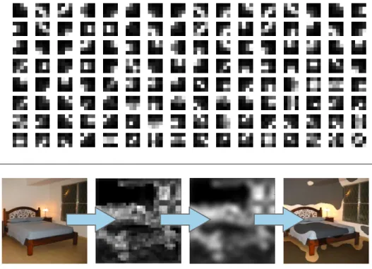
In Fig. 2 we visualize the 128 SIFT Independent Components (as computed from one training split of the ISR [23] dataset), together with an example of how a SIFT Saliency map is formed, and a comparison of the resulting histograms with other pooling strategies. As expected, this saliency operator is taking into account only the textural information provided by the SIFT features, while disregarding other channels, like color and intensity.

3.2 Task-driven spatial pooling

So far we have defined a pooling strategy conceived to capture the structural regularities in the problem, regardless of their exact position. In this section we are going to complement it with a simple spatial pooling scheme, specifically devised for indoor scenes.

1_{For our segmentation and pooling goal we don’t need a higher resolution map, since the local descriptors are}

(5)

FORNONI, CAPUTO: SALIENCY-DRIVEN POOLING FOR INDOOR SCENE RECOGNITION NS ’ S 1 NS S 512 1024 NS ’ S 1 NS S 512 1024 L ’ R 1 L R 512 1024 U ’ D 1 U D 512 1024

Salient Pooling (Itti)

Salient Pooling (SIFT)

Vertical Pooling

Horizontal Pooling

Histogram # of non-zero words

Figure 2: Top: visualization of the 128 SIFT Independent Components, summed over the 8 orientations; white pixels correspond to high ICA (rectified) weights for the gradients in the corresponding area of the SIFT patches. Middle: Computation of a SIFT saliency map and resulting segmentation. Bottom: Histograms obtained with different pooling techniques and number of non-zero visual words in each of the two halves of the histograms: non-salient (NS) and salient (S), left (L) and right (R), up (U) and down (D).

(6)

Indoor scenes are designed to support human actions and humans have a limited range of spatial mobility. For example, humans can usually walk around a room, use objects and appliances within reach, sit on chairs, etc., but they cannot easily move from the floor to the ceiling, or access facilities if they are disposed too low, or too high in the room. This reduces the spatial variability of indoor scenes to lie mostly on the horizontal axis.

Given this prior, we expect that by pooling features in horizontal bands we will be able to capture the most consistent spatial patterns in indoor scenes. We instead expect less robust results by pooling descriptors in vertical bands. To verify this intuition we performed a first set of experiments comparing the following pooling strategies:

• Horizontal-bands pooling. In this settingsR1is the set of local descriptors lying in the

upper 50% of the image, andR2is its complement

• Vertical-bands pooling. In this caseR1consists of the left-side 50% of the descriptors, andR2is again its complement

A visualization of these pooling strategies, with the resulting histograms is shown in Fig.2. Once the spatial and the saliency-driven encoding have been computed, we concatenate the two encodings, thus creating an image descriptor which exploits both the spatial and the structural consistencies of the scenes, and whose experimental performances are discussed in details in the following section. A multiresolution version [7] of our image descriptor is also formed by down-sampling each image by a factor of two, and concatenating the histograms obtained at the two resolutions.

4 Experiments

In order to assess the effectiveness of our approach, we performed experiments on three widely used scene recognition datasets: (1) the Indoor Scene Recognition (ISR) dataset [23], consisting of 15620 images collected from the web and belonging to 67 different indoor categories, with a minimum of 100 images per category; (2) the 15-Scenes [13] dataset, containing 4485 low-resolution and gray-valued images, from indoor and outdoor categories; (3) the 8-Sports dataset [15], collecting images of eight sports, with a number of images per category between 137 and 250. In all experiments we compare the performance of our approach with different spatial pooling baselines, and we also analyze the relative importance of its sub-components: the salient and the spatial pooling schemes. In the following we first describe the experimental setup, we then present results for the ISR dataset, and we finally show the performance on the other two datasets.

4.1 Experimental setup

We extract SIFT2descriptors on a grid with 8 pixels spacing and with a patch size of 16×16 pixels. When computing the multiresolution description, the spacing and patch size for the downsampled images are reduced to 6 and 12×12. For each resolution, a vocabularyBwith

M=1024 visual words is obtained by running k-means on a random subset of the training features, and the same set of features is used to learn the ICA basis. The intermediate image representationCis then obtained using approximated unconstrained LLC encoding [27], withK=5. Since the importance of each visual-word for the reconstruction of a SIFT

(7)

FORNONI, CAPUTO: SALIENCY-DRIVEN POOLING FOR INDOOR SCENE RECOGNITION Resolution 1 Resolution 1+2 30 35 40 45 50 55 Accuracy %

Indoor Scene Recognition dataset

L0 Vertical Saliency Itti Saliency SIFT Horizontal Horizontal + Vertical Horizontal + Saliency Itti Horizontal + Saliency SIFT L1

L2 L3

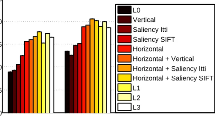
Figure 3: Performances of the different pooling strategies on the ISR dataset.

point is given only by the magnitude of its response, and to avoid cancellation effects with average-pooling, we also perform rectification of the codewords responsesci, using abs(ci).

AfterR1andR2have been defined, we separately`1-normalize each of the two histograms

¯

cR1 and ¯cR2, obtained by average pooling. This ensures that images with different sizes will contribute to the learning in the same way, and that the two regions will have exactly the same importance in the final representation. This inner-normalization is not performed on theL1,L2 andL3 baselines to avoid emphasizing the histograms computed on small patches; in this case we perform the`1-normalization on the full vector only. As a similarity measure

for all our histograms we make use of the exponentialχ2kernel [4], withγset to the average

pairwiseχ2distance between the training samples, as in [6]. The classification is finally

performed using SVM [3], withCfixed to 100 for all the features and datasets.

With this setup any single region is represented by a 1024-dimensional histogram, so that for example, the standardL3 pyramid representation results in a 87040-dimensional de-scriptor, while a Spatial + Salient pooling approach results in a 4096-dimensional descriptor. Natural baselines for our Spatial + Salient pooling approach are the Horizontal + Vertical (4096-dimensional) and theL1 (5120-dimensional) pooling strategies.

4.2 Results on indoor scenes

The standard benchmarking procedure for the ISR dataset consists of randomly selecting 100 images per category and split them into 80 images for training and 20 for testing. We repeated the experiment on five random training/test split and we report the average classifi-cation accuracy in Fig.3.

We see that there is a large difference in performance between the horizontal and the vertical pooling strategies (+16.2% relative improvement, on the single resolution). This is not really surprising considering the spatial structure of the problem. The salient pooling strategies perform better than the vertical (+8.1%), but still worse than the horizontal one. On the other hand, when combined with the horizontal pooling, they always outperform the Horizontal + Vertical and theL1 baselines, being also competitive with much higher dimen-sional representations likeL2 andL3. On this dataset the SIFT saliency seems to outperform the Itti operator. However, when combined with the horizontal pooling, or at multiple reso-lution, the differences dwindle. This could be explained by examining Fig. 4-right, where

(8)

Vertical Horizontal Saliency Saliency SIFT

0 100 200 300 400 500 600 700 800 900 L R U D NS S NS S Average Number of no n−zero bins

Average Number of non−zero bins, on the ISR dataset

0 10 20 30 40 50 60 70

Overlap (% of image pixels)

Average overlap of pooling regions, on the ISR dataset

Itti Saliency, Horizontal Itti Saliency, Vertical SIFT Saliency, Horizontal SIFT Saliency, Vertical Itti Saliency, SIFT Saliency

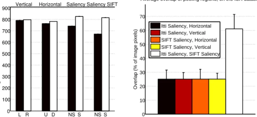
Figure 4: Left: average number of non-zero visual words in each part of the representation, as obtained with different pooling techniques. Right: average overlap (in % of the number of pixels) between salient regions and horizontal/vertical patches, compared to the average overlap of the salient regions obtained with the Itti and the SIFT saliency operators. All measures have been obtained on the ISR dataset.

we plot the average overlap between salient regions and horizontal/vertical patches. We see that the Itti and the SIFT saliency operators produce segmentations which overlap for more than 60% of the pixels, thus resulting in quite similar image descriptions. In the same figure we also plot the average overlap of the two (Itti and SIFT) salient regions, with the horizon-tal/ vertical patches, showing it to be exactly of 25% of the pixels: on average, only half of the salient region overlaps with the upper/lower, or left/right regions (a salient region in-cludes by design 50% of the pixels). This confirms the fact that the salient pooling captures information that is not spatially biased.

In Fig. 2and Fig. 4-left we also plot the number of non-zero visual words in each part of the representation. This measure is related to the visual complexity of the area being described: a very complex (part of a) scene is expected to generate a high number of re-sponses to many different visual words, while less complex areas are expected to generate highly peaked histograms, with only few active visual words. We see that the saliency-driven pooling approaches produce a representation where the most complex areas of the image are pooled together in the salient region, while the least complex ones end up in the non-salient set. This contrasts with the canonical spatial encodings, where the consistency is only in the absolute position of the features. Finally, Table1 compares the performances of our descriptors with other state of the art approaches: for the ISR dataset, we are state of the art.

4.3 Results on other scene categorization tasks

Our approach has been specifically designed to address the high intra-class spatial variabil-ities of indoor scenes. In this section we are going to verify experimentally how well this approach generalizes to other scene recognition problems.

For the 15 Scenes dataset we followed the standard benchmarking protocol, which con-sists in randomly selecting 100 training images per class and using the remaining ones for the test. For the Sports dataset the standard procedure consists instead in selecting 70 images per class for the training set, and the remaining 60 for the test set. We repeated the experiments five times and we report the average classification accuracy in Fig.5.

(9)

FORNONI, CAPUTO: SALIENCY-DRIVEN POOLING FOR INDOOR SCENE RECOGNITION Resolution 1 Resolution 1+2 70 72 74 76 78 80 82 84 86 88 90 Accuracy % 15−Scenes dataset L0 Vertical Saliency Itti Saliency SIFT Horizontal Horizontal + Vertical Horizontal + Saliency Itti Horizontal + Saliency SIFT L1 L2 L3 Resolution 1 Resolution 1+2 70 72 74 76 78 80 82 84 86 88 90 Accuracy % Sports dataset L0 Vertical Saliency Itti Saliency SIFT Horizontal Horizontal + Vertical Horizontal + Saliency Itti Horizontal + Saliency SIFT L1

L2 L3

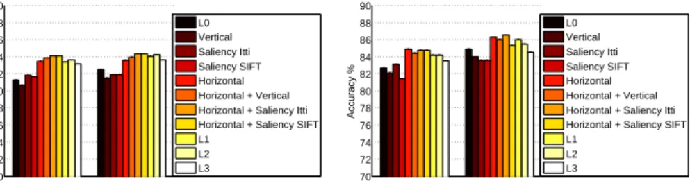
Figure 5: Performances on the 15 Scenes (left) and the Sports (right) datasets

Method ISR 15 Scenes Sports

Quattoni and Torralba [23] 2009 25.05 -

-Zhou et al. [30] 2009 - 85.2

-Li et al. [14] 2010 37.6 80.9 76.3

Morioka and Satoh [18] 2010 39.6 83.40

-Pandey and Lazebnik [21] 2011 43.1 -

-Nakayama et al. [19] 2010 45.5 86.1 84.4

Cakir et al. [2] 2011 47.01 82.24

-Wu and Rehg [28] 2011 - 83.10 85.65

Our approach (Itti) 46.64 84.14 84.75

Our approach (SIFT) 47.73 84.12 84.75

Our approach Multiresolution (Itti) 50.54 84.37 86.54

Our approach Multiresolution (SIFT) 50.16 84.39 85.29

Table 1: Performance comparison with previous studies.

We see that the results on the 15 Scenes dataset are consistent with what we obtained on the ISR dataset, even if with a lower gain in performance. However, on the Sports dataset the SIFT salient pooling is performing consistently worse than the one based on Itti’s saliency. One possible explanation might be that the former operator only takes into account the tex-tural property of the scene, which might not be useful for consistently separating the scene foreground (e.g., a group of people rowing), from a highly textured natural background (e.g., vegetation, water and buildings). It should also be noted that this dataset is the most di-verse with respect to our initial indoor scene categorization task and that the multiresolution Horizontal + Saliency Itti pooling approach still achieves the state of the art (see Table1).

5 Conclusions

In this paper we proposed a saliency-driven feature pooling technique able to capture per-ceptually coherent structures, independently from their imaged position. We made use of a well-known saliency operator and proposed a new saliency function, directly employing the rich information encoded in the local descriptors to obtain the saliency map. The de-rived image representation, combined with a simple task-driven spatial pooling, results in a descriptor that obtains state of the art performances on the ISR and Sports datasets, while being still competitive on the 15 Scenes collection. Furthermore, the resulting feature vector is up to an order of magnitude smaller compared to existing approaches [13].

(10)

Acknowledgements This work was partially supported (M.F.) by the SNF grant ICS -Interactive Cognitive Systems.

References

[1] N. Bruce and J. Tsotsos. Saliency based on information maximization.Proc. Advances in Neural Information Processing Systems, 18:155, 2006.

[2] F. Cakir, U. Güdükbay, and Ö. Ulusoy. Nearest-neighbor based metric functions for indoor scene recognition. Computer Vision and Image Understanding, 2011.

[3] Chih-Chung Chang and Chih-Jen Lin. LIBSVM: A library for support vector ma-chines.ACM Transactions on Intelligent Systems and Technology, 2:27:1–27:27, 2011.

Software available athttp://www.csie.ntu.edu.tw/~cjlin/libsvm.

[4] C. Fowlkes, S. Belongie, F. Chung, and J. Malik. Spectral grouping using the Nyström method.IEEE Transactions on Pattern Analysis and Machine Intelligence, pages 214– 225, 2004. ISSN 0162-8828.

[5] D. Gao and N. Vasconcelos. Integrated learning of saliency, complex features, and ob-ject detectors from cluttered scenes. InProc. Computer Vision and Pattern Recognition, volume 2, pages 282–287. IEEE, 2005.

[6] P. Gehler and S. Nowozin. On feature combination for multiclass object classification. InProc. International Conference on Computer Vision, volume 1, page 6, 2009. [7] E. Hadjidemetriou, M.D. Grossberg, and S.K. Nayar. Multiresolution histograms and

their use for recognition. Pattern Analysis and Machine Intelligence, IEEE Transac-tions on, 26(7):831–847, 2004.

[8] T. Harada, Y. Ushiku, Y. Yamashita, and Y. Kuniyoshi. Discriminative spatial pyramid. InProc. Computer Vision and Pattern Recognition, pages 1617–1624. IEEE, 2011.

[9] J. Harel. A saliency implementation in matlab @ONLINE, 2006. URL http://

www.klab.caltech.edu/~harel/share/gbvs.php.

[10] X. Hou, J. Harel, and C. Koch. Image signature: Highlighting sparse salient regions.

IEEE Transactions on Pattern Analysis and Machine Intelligence, 34(1):194, 2012. [11] A. Hyvärinen and E. Oja. Independent component analysis: algorithms and

applica-tions.Neural networks, 13(4-5):411–430, 2000.

[12] L. Itti, C. Koch, and E. Niebur. A model of saliency-based visual attention for rapid scene analysis. Pattern Analysis and Machine Intelligence, IEEE Transactions on, 20 (11):1254–1259, 2002. ISSN 0162-8828.

[13] S. Lazebnik, C. Schmid, and J. Ponce. Beyond bags of features: Spatial pyramid matching for recognizing natural scene categories. InProc. Computer Vision and Pat-tern Recognition, volume 2, 2006.

(11)

[14] L. Li, H. Su, E. P. Xing, and L. Fei-Fei. Object Bank: A High-Level Image Represen-tation for Scene Classification and Semantic Feature Sparsification. InProc. Neural Information Processing Systems, 2010.

[15] L.J. Li and L. Fei-Fei. What, where and who? classifying events by scene and object recognition. InProc. International Conference on Computer Vision, pages 1–8. IEEE, 2007.

[16] D.G. Lowe. Distinctive image features from scale-invariant keypoints. International journal of computer vision, 60(2):91–110, 2004.

[17] F. Moosmann, D. Larlus, and F. Jurie. Learning saliency maps for object categorization. InECCV Workshop on the Representation and Use of Prior Knowledge in Vision, 2006. [18] N. Morioka and S. Satoh. Building compact local pairwise codebook with joint feature space clustering. Proc. European Conference on Computer Vision, pages 692–705, 2010.

[19] H. Nakayama, T. Harada, and Y. Kuniyoshi. Global gaussian approach for scene cate-gorization using information geometry. InProc. Computer Vision and Pattern Recog-nition, pages 2336–2343. IEEE, 2010.

[20] A. Oliva and A. Torralba. Modeling the shape of the scene: A holistic representation of the spatial envelope. International Journal of Computer Vision, 42(3):145–175, 2001. ISSN 0920-5691.

[21] M. Pandey and S. Lazebnik. Scene recognition and weakly supervised object localiza-tion with deformable part-based models. InProc. International Conference on Com-puter Vision, pages 1307–1314. IEEE, 2011.

[22] D. Parikh, C. Zitnick, and T. Chen. Determining patch saliency using low-level context.

Proc. European Conference on Computer Vision, pages 446–459, 2008.

[23] A. Quattoni and A. Torralba. Recognizing indoor scenes. InIn Proc. Computer Vision and Pattern Recognition. IEEE, 2009.

[24] K. Rapantzikos, N. Tsapatsoulis, Y. Avrithis, and S. Kollias. Spatiotemporal saliency for video classification. Signal Processing: Image Communication, 24(7):557–571, 2009. ISSN 0923-5965.

[25] G. Sharma, F. Jurie, and C. Schmid. Discriminative spatial saliency for image classifi-cation. InProc. Computer Vision and Pattern Recognition, 2012.

[26] K.N. Walker, T.F. Cootes, and C.J. Taylor. Locating salient object features. InProc. British Machine Vision Conference, volume 2, pages 557–566. Citeseer, 1998. [27] J. Wang, J. Yang, K. Yu, F. Lv, T. Huang, and Y. Gong. Locality-constrained linear

coding for image classification. InComputer Vision and Pattern Recognition, pages 3360–3367. IEEE, 2010.

[28] J. Wu and J.M. Rehg. Centrist: A visual descriptor for scene categorization. Pattern Analysis and Machine Intelligence, IEEE Transactions on, 33(8):1489–1501, 2011.

(12)

[29] L. Zhou, D. Hu, Z. Zhou, and Z. Zhuang. Natural scene recognition using weighted histograms of gradient orientation descriptor. Frontiers of Electrical and Electronic Engineering in China, 6(2):318–327, 2011.

[30] X. Zhou, N. Cui, Z. Li, F. Liang, and T.S. Huang. Hierarchical gaussianization for image classification. InProc. International Conference on Computer Vision, pages 1971–1977. IEEE, 2009.