Sequential optimization for efficient high-quality object proposal generation

OpenBU

http://open.bu.edu

BU Open Access Articles BU Open Access Articles

2018-05-01

Sequential optimization for efficient

high-quality object proposal

generation

This work was made openly accessible by BU Faculty. Please

share

how this access benefits you.

Your story matters.

Version

Citation (published version): Ziming Zhang, Yun Liu, Xi Chen, Yanjun Zhu, Ming-Ming Cheng,

Venkatesh Saligrama, Philip HS Torr. 2018. "Sequential Optimization

for Efficient High-Quality Object Proposal Generation." IEEE

Transactions On Pattern Analysis And Machine Intelligence, Volume

40, Issue 5, pp. 1209 - 1223 (15).

https://doi.org/10.1109/TPAMI.2017.2707492

https://hdl.handle.net/2144/29424

Sequential Optimization for Efficient High-Quality

Object Proposal Generation

Ziming Zhang, Yun Liu, Xi Chen, Yanjun Zhu, Ming-Ming Cheng, Venkatesh Saligrama, and Philip H.S. Torr

Abstract—We are motivated by the need for a generic object proposal generation algorithm which achieves good balance between object detection recall, proposal localization quality and computational efficiency. We propose a novel object proposal algorithm,BING++, which inherits the virtue of good computational efficiency of BING [1] but significantly improves its proposal localization quality. At high level we formulate the problem of object proposal generation from a novel probabilistic perspective, based on which our BING++ manages to improve the localization quality by employing edges and segments to estimate object boundaries and update the proposals sequentially. We propose learning the parameters efficiently by searching for approximate solutions in a quantized parameter space for complexity reduction. We demonstrate the generalization of BING++ with the same fixed parameters across different object classes and datasets. Empirically our BING++ can run athalfspeed of BING on CPU, but significantly improve the localization quality by 18.5% and 16.7% on both VOC2007 and Microhsoft COCO datasets, respectively. Compared with other state-of-the-art approaches, BING++ can achieve comparable performance, but run significantly faster.

Index Terms—Efficient high-quality object proposal, Object detection, Sequential minimization

F

1 INTRODUCTION

G

standalone preprocessing step in many applications such as object recognition [2] and detection [3], and conse-quently has attracted significant attention. Object proposal generation can be broadly measured using three metrics: (a)

Detection Recall(DR) [1], [4], [5], which is the ratio between

the number of correctly detected objects and the total

num-ber of objects in the dataset; (b)Proposal Localization Quality

in terms of average best overlap (ABO) for each object instance in each class, and corresponding mean average best

overlap (MABO) across all the classes [6]; (c)Computational

Efficiency(CE). In this paper, we are interested in developing

new algorithms to provide a small set of windows (i.e.

bounding boxes) in images with high DR, high localization quality (especially for MABO), and high CE.

In recent years while many object proposal generation algorithms have been proposed, existing methods do not appear to achieve good balance between DR, MABO and CE. Fig. 1 depicts inherent tradeoffs in DR, MABO and CE among different proposal algorithms. We can see clearly that, for instance, BING [1] is computationally efficient but has poor localization quality, while selective search [6] generates good proposals but is computationally inefficient. Our perspective here is that computational efficiency has to be an important consideration in developing algorithms

• Dr. Z. Zhang is with Mitsubishi Electric Research Laboratories (MERL), Cambridge, MA 02139-1955, U.S. E-mail: [email protected] • Y. Liu and Prof. M-M. Cheng are with CCCE & CS, Nankai Uni-versity, Tianjin 300071, China. E-mail: [email protected], [email protected]

• X. Chen and Y. Zhu are with the School of Automation, Huazhong University of Science and Technology, Wuhan 430074, China. E-mail: {chenxihust, yjzhu}@hust.edu.cn,

• Prof. V. Saligrama is with the Department of Electrical and Computer Engineering, Boston University, Boston, MA 02215, US. E-mail: [email protected]

• Prof. P.H.S. Torr is with the Department of Engineering Sci-ence, University of Oxford, Oxford OX1 3PJ, UK. E-mail: [email protected]

(a) DR vs. computational time (b) MABO vs. computational time

Fig. 1. Comparison of generic object proposal methods on

VOC2007 test dataset [7] with at most 1,000 proposals per image and intersection-over-union (IoU) threshold equal to 0.5. All the competing results are produced by public code (see Table 3 and 4 in Section 4 for more details).

since object proposal generation is typically a preprocessing step. Based on this reasoning, we propose a novel object

proposal algorithm,BING++, which is an extension of our

previous work [1], [4], [5].

Fig. 2. Best overlap (BO)

statistical comparison using at most 1,000 proposals per im-age and IoU threshold 0.5 on VOC2007 test dataset.

BING [1] has been demon-strated as a very efficient ob-ject proposal algorithm. Its basic idea is to first train lin-ear filters for each so-called

quantized scale/aspect-ratio (or

quantized window size) [4], [5] using simple binary gra-dient features, and then learn another global linear filter to rank bounding boxes from each quantized scale/aspect-ratio and output proposals from the top list. The quan-tization scheme guarantees to

map every possible object scale/aspect-ratio to at least one

of thepredefined and fixedquantized scales/aspect-ratios. As

stated in [5], this quantization scheme reduces the pro-posal searching space logarithmically, leading to very high computational efficiency. However, this step also leads to

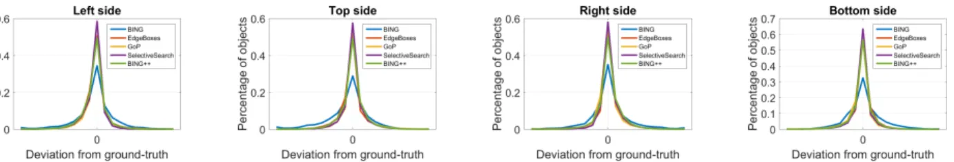
significant degradation in proposal quality in practice. To see this, here we will show some statistics about the proposal quality on VOC2007 test set. The behavior on either training or test set is similar. We first point to the best overlap (BO) statistics in Fig. 2, where we notice that the localization quality of BING proposals (over the dataset) is mediocre, because there is a clear leftward drift in BING’s distribution relative to other methods. This is indicative of poor proposal localization quality of BING. In order to see how proposals drift from the ground-truth, we point to comparison between the boundary deviation statistics based on percentage of objects and the best proposal deviation from the ground-truth bounding box per object in Fig. 3. Ideally a Dirac delta distribution in this context is preferable, and the closer the distribution to Dirac delta, the better the proposal algorithm in terms of localization quality. Com-pared to other competitors, BING performs worse because its distributions appear to have heavier tails on both sides. This indicates that BING is agnostic between choosing larger or smaller proposals for the ground-truth.

On the other hand since BING has high DR, we conclude

that the quantization scheme in BING leads to poor proposal

localization quality. We infer this based on the view that

BING does not allow the proposals to be adaptive to the object boundaries. In contrast, the methods that fully utilize

either edge information (e.g. [8]) or segments/superpixels

(e.g.[6]) perform better than BING, but run much slower.

Contributions:In this paper we propose afast yet accurate

ob-ject proposal algorithm, BING++1, which inherits the virtues

of BING,i.e.computational efficiency and objectness scores,

but significantly improves its proposal localization quality. For instance, on VOC2007 BING++ achieves 77.5% in terms

of MABO with significant improvement of18.5%over BING

within only about3mson our server with two INTEL XEON

E5 2696v2 [email protected]. To our best knowledgeBING++

is the fastest object proposal algorithm among those that produce state-of-the-art quality.

We first propose a novel probabilistic perspective for understanding the problem of object proposal generation, where we reveal the nature of recursive updating mecha-nism of proposals by alternating optimization of estimating object boundaries and updating proposals accordingly. This probabilistic view can be served as the theoretical justi-fication of our BING++ (as well as some other proposal algorithms such as [9]). We learn the corresponding pa-rameters efficiently by searching for approximate solutions in a quantized parameter space for complexity reduction. We demonstrate the robustness of such learned parameters across different datasets. In reality we utilize edges and seg-ments sequentially to estimate object boundaries as guide to update proposals further. In such way BING++ manages to improve the localization quality recursively in a coarse-to-fine manner. We test BING++ on VOC2007 and Microsoft COCO [10] datasets, and consistently achieve better trade-off between DR, MABO, and CE, compared with many other object proposal generation algorithms.

1.1 BING for Objectness Measure

Objects are typically considered as stand-alone things with well-defined closed boundaries and centers [11]. When

re-1. The code is available at https://zimingzhang.wordpress.com/.

sizing windows corresponding to real world objects to a

small fixed size (e.g.8×8), the norm (i.e.magnitude) of the

corresponding image gradients becomes a good discrimina-tive feature, due to the little variation that closed boundaries could present in such abstracted views. Also inspired by the ability of human vision system which efficiently per-ceives objects before identifying them [12], we introduce a

simple 64-dim normed gradient (NG) feature as well as its

approximation,i.e. binarized normed gradient (BING)feature,

for efficiently capturing the objectness of an image window. To find generic objects in an image, we scan over

pre-definedquantized window sizes(scales and aspect ratios) [4],

[5]. Each window is scored with a linear modelw∈R64:

sl=hw,gli, l= (i, x, y), (1)

where sl, gl, l, i and (x, y) are filter score, NG feature,

location, size and position of a window respectively, and

h·,·i denotes the inner product operator of two vectors.

Using non-maximal suppression (NMS), we select a small

set of proposals from each sizei. Some sizes (e.g.10×500)

are less likely than others to contain an object instance (e.g.

100×100). Thus we define the objectness score (i.e.calibrated

filter score),cl, as

cl=visl+ti, (2)

where vi, ti ∈ R are separately learned coefficient and a

bias terms for each quantized sizei. Note that calibration

based on Eq. 2, although very fast, is only required when re-ranking the small set of final proposals.

To make use of recent advantages in model binarization approximation [13], [14], we propose an accelerated version

of NG features,i.e.BING, to speed up the feature extraction

and testing process. Our learned linear modelw∈R64 can

be approximated with a set of basis vectorsw≈PNw

j=1βjaj

using [13], whereNw denotes the number of basis vectors,

aj ∈ {−1,1}64 denotes a basis vector, andβj ∈Rdenotes

the corresponding coefficient. By further representing each

ajusing a binary vector and its complement:aj=a+j −a

+ j,

wherea+_j ∈ {0,1}64

, a binarized featurebcould be tested

using fastBITWISE ANDandBIT COUNToperations (see [13]),

hw,bi ≈XNw

j=1βj(2ha +

j,bi − |b|). (3)

We approximate the NG values (each saved as a BYTE

value) using the topNgbinary bits of theBYTEvalues. Thus,

a 64-dim NG featureglcan be approximated byNg(BING)

features as gl= XNg k=12 8−k bk,l, (4)

where bk,l,∀k,∀l is a binarized feature. Note that these

BING features have different weights based on their bit

positions inBYTEvalues. Accordingly the filter score in Eq. 1

of a window corresponding to BING feature bk,l can be

efficiently tested using:

sl≈

XNw j=1βj

XNg

k=1Cj,k, (5)

whereCj,k = 28−k(2ha+j,bk,li − |bk,l|)can be tested using

fast BITWISE and POPCNT SSE operators. For more details please refer to our paper [1].

Fig. 3. Statistical comparison based on percentage of objectsvs.best proposal deviation from the ground-truth bounding box per object with at most 1,000 proposals per image and IoU threshold 0.5 on VOC2007 test dataset.

1.2 Related Work

Object proposal generation algorithms for images in the literature can be further categorized into three groups, in general, as follows:

(i) Segmentation/Superpixel based algorithms: In fact most

proposal generation algorithms fall into this group. For instance, objectness measure [15] combines saliency, color, edges, and superpixels to score the windows, and then sam-ples bounding boxes with high scores as object proposals.

Based on [15], Rahtuet al.[16] proposed another cascaded

method, where the proposal candidates are sampled from super-pixels based on a prior object localization distribution and then ranked using structured learning with learned

fea-tures. Further in [17], Blaschkoet al.investigated the effect of

the NMS step in [16] to improve the performance. Uijlingset

al.[6] proposed selective search by combining the strength

of both an exhaustive search and segmentation and being

guided by the image structure. Manenet al.[18] proposed a

randomized Prim algorithm on the superpixel connectivity graphs. Endres and Hoiem [19] proposed ranking the a set of segments using structured learning based on various cues. Krähenbühl and Koltun [20] proposed identifying crit-ical level sets in geodesic distance transforms as proposals, and in [21] they proposed learning ensembles of classifiers for generating proposals. There are several methods based on energy minimization, such as constrained parametric min-cut [22], [23], RIGOR [24], and parametric min-loss [25]. Some other methods utilized segmentation/superpixel grouping using, for instance, segment hierarchy [26], [27], [28], [29] or new distance measure [30]. In general, most of these methods can achieve good localization quality, but suffer from either poor computational efficiency or low DR during testing.

(ii) Edge based algorithms: Compared with segments and

superpixels, edges are lightweight visual features in terms of computation. Currently most of the efficient proposal

algo-rithms utilize edge related features. Zhanget al.[4] proposed

a cascaded ranking SVM (CSVM) method to sample the proposals based on image gradients in a sliding-window manner, and later generalized the method into two-stage

cascade SVMs in [5]. Cheng et al. [1] proposed the BING

algorithm with binary features running at 300fps. Zhaoet al.

[31] showed that the success of BING is rather in combina-torial geometry and proposed a window sampling method accordingly. Zitnick and Dollár [8] proposed the EdgeBoxes algorithm to fast generate proposals based on edges and

contours while achieving good localization quality. Luet al.

[32] proposed a contour box algorithm to reject the object proposals without explicit closed contours. In addition,

Qi et al. [33] proposed a perceptual grouping framework

that organizes image edges into meaningful structures, and tested this method for object proposal generation. Ghodrati

et al.[34] proposed a DeepProposal method based on

convo-lutional neural networks (CNN). Renet al.[35] proposed the

region proposal network (RPN) to accelerate the fast R-CNN [35] for object detection. In general, edge based algorithms are faster than segmentation based algorithm. Among them, BING is the fastest in the literature, but suffers from poor proposal localization quality seriously.

(iii) Proposal post-processing:Several recent works focus on

improving proposal quality with small amount of compu-tational cost. For instance, He and Lau [36] proposed an oriented object proposal algorithm for better locating objects

by estimating their orientations. Wang et al. [9] proposed

using multi-thresholding straddling expansion (MTSE) to improve quality using superpixels.

A comprehensive comparison between some different object proposal algorithms can be found in [37]. In contrast, our BING++ utilizes both edge and segmentation informa-tion sequentially to improve the proposal quality gradually, achieving better trade-off between proposal quality and computational efficiency in the literature.

2 UNDERSTANDING OBJECT PROPOSALS: A PROB

-ABILISTICPERSPECTIVE

Let us consider the training (if any) and testing procedures separately for an object proposal algorithm. We denote

as {xi}i=1,···,N the training data with N images, and as

{sij}j=1,···,Ni,∀i the ground-truth bounding box

coordi-nates (i.e. sij ∈ R4) for Ni objects in the i-th image,

one box per object. Given a proposal quality measureoand

a corresponding threshold η ≥ 0, the training goal of a

proposal algorithm is to determine a suitable structured

predictionfunction (or mapping rule), f∗, to maximize the

likelihood of correct detections (or equivalently) as follows:

f∗= arg max f∈F N Y i=1 Ni Y j=1 P max y∈f(xi) o(y,sij)≥η xi,sij , (6)

wheref:x→ Y ⊆R4 is the proposal generation function

(or more generally an algorithm) from a feasible functional

space F that extracts a collection of potential object

re-gions Y as proposals from image x, and P denotes the

conditional probability. Here functiono(y,sij)measures the

overlap (e.g.using intersection-over-union (IoU)) between a

proposaly and the ground-truthsij. If this value is larger

thanη(e.g.η= 0.5) we consider this proposal as acorrect

de-tection for the object. Then the likelihood in Eq. 6 essentially measures the joint probability of overall correct detections among the entire training data, which should be maximized

by functionf∗. Note that the functional space F could be

restricted by certain (regularization) requirements such as number of proposals. For simplicity we do not explicitly show these requirements in the objective but assume that

for the other functional spaces in the rest of the paper, we make the same assumption without explicit mention.

Recently researchers in computer vision have started to investigate the learning problems with such complicated quality measure [38], [39]. For instance, Nowozin in [38] studied the problem of making optimal decisions from probabilistic models with IoU scores and proposed a greedy algorithm to efficiently solve it. In contrast our learning problem in Eq. 6 (and similarly in the related equations latter) can be potentially generalized to an arbitrary overlap measure with specific algorithms developed for generic object proposal generation (see Section 3).

In test time we would like to generate proposals for possible objects in test images using the learned function

f∗. As we see in Fig. 2, there are very small portions of

objects having best overlap (BO) scores less thanη = 0.5,

indicating that the training procedure withη = 0.5 works

well. However, with the increase of thresholdη, say to 0.7,

as a new decision rule for correct detection, it is clear that for BING there will be a large portion of proposals which are considered as wrong detections.

In order to solve this performance degradation problem, one possible solution is to retrain the models in Eq. 6 directly with higher thresholds. This strategy, however, becomes more and more difficult with the increase of the threshold (see the experimental evaluation in [4], [5]), because in real data the parameter space for ground-truth bounding boxes of objects is so huge that localizing such windows accurately is extremely difficult with consideration of computational efficiency.

Alternating optimization:Another possible solution is to

pre-sume that the feasible functional spaceF has certain

struc-tures, so that we can shrink the searching space in F,

leading to much lower model complexity. Similar ideas have been explored in many different research areas, for instance, recently in developing efficient algorithms for training deep neural networks [40], where circulant structures are used to simplify the fully-connected layers.

Particularly, in this paper we presumeFas the

composi-tion of funccomposi-tional spaces as follows:

F def=F1× F2× · · · × FM−1× FM, (7)

where Fm,∀m = 1,· · ·, M denotes a feasible functional

space. Accordingly we can view function f∗ as the

com-position of functions as follows:

f∗def=fM∗ ◦f ∗ M−1◦ · · · ◦f ∗ 2 ◦f ∗ 1, (8)

where fm∗,∀m = 1,· · ·, M denotes the m-th atomic

local-ization function which is applied sequentially to generate

proposals. A good example based on such methodology is [9], where a superpixel merging technique was applied on top of existing proposal generators to improve localization quality. Considering the problem in Eq. 6, such solutions

from Eq. 8 are always suboptimal (with local optimality at

fm∗ in each functional spaceFm).

Intuitively this function composition in Eq. 8 suggests an alternating optimization routine to learn such atomic functions. That is,

fm∗ = arg max fm∈Fm Y i,j P max y∈f(xi) o(y,sij)≥η xi,sij , (9)

wherefdef= fM∗ ◦ · · · ◦fm◦ · · · ◦f1∗,∀mwith the other fixed

learned functions such asf1∗andfM∗. Actually in our work

[41] we have explored similar ideas and proposed a specific alternating optimization algorithm for learning these filters in cascade SVMs.

Sequential optimization: The main challenge of developing

such alternating optimization algorithms for proposal gen-eration lies in the fact that mathematical formulation of such ad hoc algorithms is extremely difficult to propose. Instead for simplicity in practice the atomic functions in these algorithms are usually learned/designed sequentially, such as [9]. Consequently this leads to the learning rule as

fm∗ = arg max fm∈Fm Y i,j P max y∈fm( ¯fm∗(xi)) o(y,sij)≥η xi,sij , (10) wheref¯m∗ def = fm∗−1◦ · · · ◦f ∗

1,∀mis a fixed function that can

be learned by solving Eq. 10 recursively form−1 times.

Obviously the maximum likelihood learned based on Eq. 10 is the lower bound of that based on Eq. 9 and thus Eq. 6.

In fact the training approach in our previous work [4], [5] as well as BING [1] is an exemplar that falls in this lower bound

sequential maximization scheme.First we learn a linear filter

for each quantized scale/aspect-ratio in image space, and then on top of the filter responses we learn a second linear filter for final ranking purpose across different quantized scales/aspect-ratios. Here we take any feature from a win-dow whose overlap with a ground-truth bounding box is

larger than thresholdη as a positive instance for learning,

otherwise as a negative one instead.

3 BING++

As we state before, due to thefixed and unadaptive

quan-tization scheme, BING can only be considered as acoarse

proposal generator. The goal of BING++ is to learn more

functionssequentiallyon top of BING to refine its proposals

efficiently and effectively. Note that the proposed method can also be applied on top of other proposal generation

al-gorithms for refinement purpose. In order to achieve thebest

trade-off between localization quality and computational efficiency, we propose BING++ as our algorithm.

To parameterize Eq. 10 for sequential optimization, in this paper we choose to utilize Gaussian distributions with the

0/1-loss function to model the likelihoodP that maximizes

DR givenη. Other parameterizations may also be applied

here,e.g. maximizing MABO using Gaussian distributions

with the least square loss and η = 1, but how to select

parameterization is beyond the scope of this paper. In

summary, we parameterizeP in Eq. 10 as follows:

P def= exp −1n max_{y∈fm( ¯f}∗ m(xi))o(y,sij)<η o , (11) wheref¯m∗ def =fm∗−1◦ · · · ◦f ∗ 1◦f ∗ B,∀m,f ∗

B denotes the learned

sequential functions by BING after training (i.e. fB∗(xi),∀i

represents the output proposals by BING for image xi),

1{·} denotes the binary indicator function measuring the

localization quality of proposals generated by functionfm,

and it returns 1 if the condition is true, otherwise 0. Then by taking the log operation on the right hand side of Eq. 10,

we can write thelog-likelihoodof Eq. 10 as follows: fm∗ = arg min fm∈Fm X i,j 1n max_{y∈fm( ¯f}∗ m(xi))o(y,sij)<η o. (12)

Recall that the goal of our BING++ is to generate object

proposals accurately as well as efficiently (i.e.fast running

speed). To achieve this goal, we propose a specific

algo-rithm, RecursiveBox, with consideration of both edge and

segment information for refining the proposals generated by BING. RecursiveBox is developed towards optimizing Eq. 12 directly, which is non-trivial, because Eq. 12 is highly non-convex. Even if we relax the 0/1-loss function

to its convex surrogate loss (e.g.hinge-loss), as traditional

methods such as SVMs, the resulting optimization problem will be still highly non-convex due to the non-convexity of

bothmaxoperator and overlap measure functiono.

To solve Eq. 12, we propose a very efficient algorithm to

search for theapproximatesolution in aquantizedparameter

space. We deliberately design functionfm for different

im-age cues (i.e.edges and segments in this paper particularly),

and quantize the corresponding parameter space into a finite number of disjoint subspaces, represented by the cen-troid parameter of each subspace (similar to cluster centers in KMeans). Then using each representative parameter, we can simply compute the loss in Eq. 12. By collecting all the losses we can select a representative parameter as the approximate solution which leads to a minimum loss.

Intuitively our RecursiveBox works as follows: At timet,

we estimate a new bounding box for objects based on both image cues and the location/scale of the current bounding box. If both bounding boxes share a large overlap, we consider the new box as a good estimator/proposal, because it is stabilizing. Otherwise, we update the current bounding

box with the new one for time t+ 1. This deterministic

rule is repeated over time until some termination criterion

(e.g. number of iterations) is satisfied. In each update we

equivalently learn a function as fm in Eq. 12 that can

be applied sequentially. Meanwhile we preserve all the objectness scores associated with the initial bounding boxes. In the following sections, we first explain how to refine proposals using edge information in Section 3.1, which is extremely computationally efficient. Then we introduce segment information as the other cue for refinement in Section 3.2, which results in higher computational burden but generates proposals with better localization quality. Finally we integrate both image cues together and propose our BING++ algorithm in Section 3.3.

3.1 Edge-based Refinement

Object proposal generation is about precisely capturing object boundaries, regardless of the pixels inside objects. We observe that good bounding boxes are those that tightly cover object boundaries. Edges as computationally efficient (compared to superpixels or segments) and indicative fea-tures to object boundaries are usually utilized to approxi-mate object boundaries [42], [43], [44]. Indeed most of the efficient proposal algorithms utilize edge related features. If the boundary of a proposal does not intersect with any edge point, we can speculate that either this proposal does not cover any object, or it is too loose. Similarly, if the proposal intersects with too many edge points, we expect that it has not yet reached the object boundary. In all of these cases, we

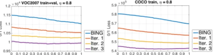
Fig. 4. Statistical behavior comparison when optimizing Eq. 15 on

VOC2007 train+val (left) and COCO training (right) datasets using

η= 0.8as the threshold for measuring high-quality proposals.

would modify the proposals by pushing them towards the

object boundaries. Therefore,we propose utilizing the nearest

edge points to proposal boundaries asfast yet weakindicators

of object boundaries to refine the proposals.

Given an image, we denote r(t) ∈ R4(t ≥ 0) as the

predicted bounding box at timet, A(r(t))⊆R2 as the set

of pixel locations in the area covered byr(t), andB ⊆R2

as the constantedge map of the image. We then generate

a pixel location set,C(r(t)), for A(r(t))by looking for the

nearest neighbors inB. That is,

C(r(t)) = q arg min q∈B d(p,q),∀p∈ A(r(t)) ⊆R2, (13)

whered(·,·) denotes a distance function. For some special

distance metric such as Euclidean distance,C(r(t))can be

efficiently computed using distance transform [45]2_.

Based onC(r(t)), we define the predicted bounding box,

r(t+ 1), at timet+ 1as follows: r(t+ 1) = (1−γ)r(t) +γ min q∈C(r(t))q;q∈Cmax(r(t))q , (14)

where min,max are entry-wise minimum and maximum

operators, [·;·] denotes the vector concatenating operator,

and0≤γ ≤1is a trade-off parameter. The basic idea of

Eq. 14 is to generate a new box by linearly integrating the two boxes.

By substituting Eq. 14 into Eq. 12, we have the following optimization problem for refining boxes based on edges:

min 0≤γ≤1 X i,j 1_{max ko(rik(t+1),sij)<η}, (15)

whererik(t+ 1),∀i,∀kdenotes thek-th new bounding box

generated from thek-th current bounding boxrik(t)in the

i-th image.

Optimization: Since the parameter γ in Eq. 15 is a scalar,

we simply enumerate all possible quantized values

as approximate solutions to accelerate the learning.

Specifically, we quantizeγ from 0 to 1, step by 0.01, and

performgreedy searchover iterations by computing the loss

in Eq. 15 based on each quantized value. Fig. 4 illustrates

the loss statistics with overlap threshold η = 0.8 (for

η >0.8 we have similar observations) because we would like to generate high-quality proposals. Note that we

learn oneγ in each iteration which results in a sequential

function that can be applied in Eq. 12. To plot these curves

we set the parameter γ for the next iteration as the one

achieving the minimum loss in the current iteration. In each iteration the inputs for the function are the outputs from the previous iteration (or BING proposals as initialization).

2. A good tutorial on how to locate the nearest edge point for each pixel using distance transform can be found at http://www. vlfeat.org/overview/imdisttf.html.

Algorithm 1EdgeRecursiveBox algorithm

Input :edge-based distance transform mapC, proposalsR,

over-lap threshold≥0

Output:improved proposalsΩ

Ω← ∅; foreachri(0)∈ Rdo fort= 0toT−1do ri(t+ 1)← minq∈C(ri(t))q; maxq∈C(ri(t))q ; ifo(ri(t),ri(t+ 1))≥thenbreak; end Ω←ΩS ri(t+ 1) end returnΩ

We repeat the same procedure to compute the overall loss in Eq. 15 on both VOC2007 train+val and COCO training datasets to verify whether we can learn the parameter with good generalization. Indeed Fig. 4 has demonstrated strong similarities between the statistical behaviors on both

datasets, suggesting that we can generalize the learned γ

values across different datasets. With increasing number of iterations the loss curves become flat on both figures, indicating the convergence of our algorithm empirically.

Implementation:We list our EdgeRecursiveBox algorithm in

Alg. 1 with computational complexity ofO(|R| ·T), roughly

speaking, where|R|denotes the number of input proposals

in set R, and T denotes the number of iterations. We

utilize canny edge detection to create edge maps B to

approximate object boundaries. Ideally accurately detecting object boundaries is very desirable yet challenging due to complex imaging factors and semantic ambiguity, and many existing works in the literature such as [42], [43], [44] followed similar ideas. Better boundary detection such as structured edges [46] may improve the proposal quality at the cost of longer computational time. We utilize Euclidean

distance for functiondin Eq. 13 and thus employ distance

transform to compute nearest edge mapsC. By taking into

account both generalization and computational complexity and based on the observation from Fig. 4, we specifically set

γ= 1, T = 3. Whenγ= 1for each iteration, the statistical

behaviors on both datasets are almost identical to those

in Fig. 4. Parameter is predefined to determine whether

the procedure of updating a bounding box converges, and

empirically we set= 0.95. In our experiments we utilize

these default values for all the datasets.

To accelerate the computation in EdgeRecursiveBox, we

resize images into1/3×1/3 = 1/9of their original sizes. The

reasons for doing are based on the observations: (1) Distance transform is relatively time-consuming, whose complexity is linearly propositional to image size. (2) Proposals hardly localize small objects correctly in the original images. In other words, discarding the detections of small objects has

little effect on localization quality measure (i.e. ABO and

MABO). Therefore, our image resizing operation leads to marginal performance degradation but significant speed-up (see our comparison in Section 4.1).

3.2 Segmentation-based Refinement

Though edges are fast to compute for approximating object boundaries, their stability is very limit. Missing boundary fragments often occur with usage of edge detection, as there is no strong contrast at such places. This will cause

(a) (b)

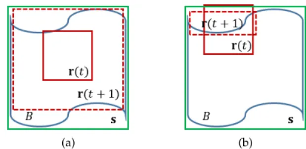
Fig. 5. Illustration of updating current red solid bounding boxr(t)

to next red dashed bounding boxr(t+ 1). Our estimation for the ground-truth bounding boxsbased onC(r(t))succeeds in (a) where the pixels inC(r(t))spread well, but fails in (b) where the pixels in C(r(t))concentrate on few boundary fragments.

serious trouble to our EdgeRecursiveBox algorithm because object boundaries cannot be inferred for precise coverage.

Also there is no guarantee that our estimatorr(t+ 1)will

approach the ground-truth bounding box eventually. Fig. 5 illustrates two simple cases where our estimation succeeds and fails, respectively, given sufficient edge information. In

(a) the current bounding box r(t) is surrounded by the

edge points in B, implying that the pixels in C(r(t)) are

sufficiently well-spread. This improves the estimate for the

ground-truth bounding box s. In (b), r(t) intersects with

the edge points. This leads to a situation whereC(r(t)) is

determined by a small fraction ofB. In practice, there may

be scenarios where the correct detections in BING could be updated to wrong bounding boxes.

To deal with these challenges in EdgeRecursiveBox, we further consider segments as a second type of useful cues which are usually more indicative of boundaries (even the coverage of objects) at the cost of more computational time. Meanwhile, bounding boxes always have overlaps with certain segments, making it possible to improve the boxes

based on the boundaries of segments. Therefore,we propose

utilizing segments as relatively slow yet strongindicators of

object boundaries to refine our proposals as well.

Given a bounding boxr(t)at timet, the training goal of

our segmentation based refinement is to learn a function (or

algorithm in general) by combining segments withr(t) to

generate a new boxr(t+ 1)so that Eq. 12 is minimized. In

test time, we apply the same function to all the bounding

boxes at time t for updating purpose. Letting S0 denote

the set of selected segments for updatingr(t), we formally

define the new boxr(t+ 1)as follows:

r(t+ 1) = min q∈A(r(t))S_A (S0₎q;_q∈A(rmax(t))S_A (S0₎q , (16)

whereA(S0)⊆R2denotes the set of pixel locations covered

by the segments inS0

.

In order to update bounding boxes using Eq. 16, intu-itively we need to find a way to select relavent segments

for S0_{. By considering this as well as minimizing Eq. 12}

we have the following general optimization problem for refining boxes based on segments:

min g∈G X i,j 1_{max ko(¯rik,sij)<η}, (17) s.t.¯rik= " min q∈A(rik(t))SA(S0ik) q; max q∈A(rik(t))SA(S0ik) q # , (18) Sik0 =g(rik(t),Si), ∀i,∀k,

0 50 100 150 200 250 300 350 400 450 500 Combination -15 -10 -5 0 5 Relative performance

×10-3 DR on VOC2007 training data, η=0.5

0 50 100 150 200 250 300 350 400 450 500 Combination -0.04 -0.03 -0.02 -0.01 0 0.01 Relative performance

MABO on VOC2007 training data

0 50 100 150 200 250 300 350 400 450 500 Combination -10 -8 -6 -4 -2 0 2 Relative performance

×10-3 DR on VOC2007 validation data, η=0.5

0 50 100 150 200 250 300 350 400 450 500 Combination -0.04 -0.03 -0.02 -0.01 0 Relative performance

MABO on VOC2007 validation data

0 50 100 150 200 250 300 350 400 450 500 Combination -10 -5 0 5 Relative performance

×10-3 DR on VOC2007 test data, η=0.5

0 50 100 150 200 250 300 350 400 450 500 Combination -0.04 -0.03 -0.02 -0.01 0 Relative performance

MABO on VOC2007 test data

Fig. 6. Statistical behavior comparison on DR/MABOvs. ∆

us-ing VOC2007 trainus-ing (top), validation (middle), and test ( bot-tom) datasets, respectively, by minimizing Eq. 17. Here x-axis shows the indexes of all possible combinations in ∆, and y-axis shows the performance improvementw.r.t.that with the combination {0.1,0.2,0.3,0.4,0.5}used in [9].

where ¯rik,∀i,∀k denotes the k-th new bounding box

generated from the k-th current bounding box rik(t) in

the i-th image, Si,∀i denotes the segment set in the i-th

image,g denotes a segment selection function to generate

the selected segment set S0

ik for rik(t), and G denotes its

feasible functional space.

Optimization: The problem in Eq. 17, in general, can be

considered as a combinatorial optimization problem [47].

However, solving Eq. 17 with an exponential number (w.r.t.

segments) of potential new boxes for each current box is extremely difficult, especially when considering computa-tional efficiency.

Instead here we utilize our parameter space quantization

mechanism again to reduce the complexity of our combi-natorial optimization problem deliberately so that we can search for corresponding new boxes efficiently as approx-imate solutions. We prefer the complexity no higher than

linear per box in terms of number of segments. To do so,

we propose grouping segments in each image into several

subsets(with overlaps) for each current bounding box and

then taking one bounding box per subset which tightly covers the corresponding segments as a new bounding box.

In such way, we can approximate the optimal gbased on

the overlap function and a set of thresholds, and further

rewrite Eq. 17 as follows:∀i,∀k,∀δ∈∆,

Sik0 =g(rik(t),Si) ={sl|o¯(sl,rik(t))≥δ,∀sl∈ Si}, (19)

where¯r(_ikδ),∀i,∀kdenotes a new bounding box at timet+ 1

parametrized by thresholdδ(0≤δ≤1)in the threshold set

∆,sl∈ Si,∀ldenotes thel-th segment in thei-th image, and

¯

o(sl,rik(t)) denotes an overlap scoring function between

segmentsland bounding boxrik(t), defined as follows:

¯

o(sl,rik(t)) =

|A(sl)∩ A(rik(t))|

|A(sl)|

∈[0,1],∀l,∀i,∀k, (20)

where A(sl) ⊆ R2,∀l denotes the set of pixel locations

covered by the segment sl, ∩ denotes the set intersection

operator, and| · |denotes the set cardinality.

Now our goal is to learn∆. To do so, we optimize Eq. 17

with Eq. 19 using nine quantization values for δ ∈ ∆, that

is, from 0.1 to 0.9, step by 0.1. Then the total number of

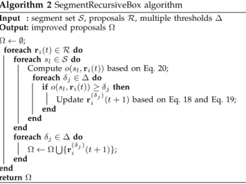
Algorithm 2SegmentRecursiveBox algorithm

Input :segment setS, proposalsR, multiple thresholds∆

Output:improved proposalsΩ

Ω← ∅;

foreachri(t)∈ Rdo

foreachsl∈ Sdo

Computeo(sl,ri(t))based on Eq. 20;

foreachδj∈∆do

ifo(sl,ri(t))≥δjthen

Updater(_iδj)(t+ 1)based on Eq. 18 and Eq. 19;

end end end foreachδj∈∆do Ω←ΩS {r(_iδj)(t+ 1)}; end end returnΩ

possible combinations for constructing∆is29_{−1 = 511,}

which are easy to be tested on the data by minimizing Eq. 17. For instance, in order to compare the statistical

behavior on localization quality (i.e.DR and MABO) using

different combinations for ∆, we show our results on

VOC2007 training, validation and test datasets in Fig. 6. We can observe clearly that the statistical behaviors on both

datasets are very similar, indicating thatthe learned threshold

set∆may have good generalization across different datasets.

Implementation: We show our SegmentRecursiveBox

algo-rithm for bounding box refinement in Alg. 2. The

compu-tational complexity of Alg. 2 isO(|R| · |∆| · |S|), roughly

speaking, where|R|,|∆|,|S|denote the numbers of

bound-ing boxes, thresholds, and segments in images, respectively. We notice that our algorithm shares many similarities with [9] in terms of implementation. However, one of the

key differences between our method and [9] is theperspective

of determining the thresholds in∆. In [9] the parameters are

fixed as [0.1,0.2,0.3,0.4,0.5] by fitting the distribution of

superpixel tightness with equal importance. As we see in Fig. 6, based on our objective the parameter combination in [9] is not the best, and many other parameter combinations can achieve very similar performance as [9]. In contrast

our method learns these parameters discriminatively by

(approximately) minimizing 0/1-loss in Eq. 17.Empirically

we set∆ ={0.1,0.3,0.6}by default for all the experiments. We employ [48] to generate segments as it can achieve good performance as well as computational efficiency. From our experiments we find that the segmentation approaches which generate segments along gradients (usually leading to larger segments) contribute significantly to the success of segmentation based box refinement algorithms such as [9]. For comparison we replace [48] with mean-shift [49] and regenerate proposals on VOC2007 test dataset. We observe slight performance degradation in such way by 1.9% and 3.8% in terms of DR and MABO, respectively. When we uti-lize mean-shift with a superpixel combination post-process,

same as the functionmeanShif tSegmentationin openCV,

our performance degrades only by 0.8% and 0.7% for DR and MABO, respectively.

As the computational complexity of [48] scales linearly with the number of input nodes in the graphs, in general, we decide to utilize “dense sampling” to generate superpixels from images as input nodes, rather than utilizing pixels

Algorithm 3Test-time BING++ for object proposals

Input :an input image I, edge based overlap threshold ≥ 0,

multiple thresholds∆, NMS parameterρ≥0

Output:generic object proposalsΩ

// BING proposals

R ←BING(I);

// edge based refinement (i.e.E-BING)

B ←CannyEdgeDetection(I);C ←DistanceTransform(B);

Ω←EdgeRecursiveBox(C,R, );

// segmentation based refinement (i.e.S-BING)

S ←Segmentation(I);Ω←SegmentRecursiveBox(S,Ω,∆);

Ω←NMS(Ω, ρ);

returnΩ

directly as did in [9], to further accelerate the computation.

Specifically we resize each image to360×400pixels, and

take every4×4pixels as a cell without overlap, leading to

90×100cells to form a grid per image. We then take each

cell as a superpixel and feed all the cells to [48]. In such way we observe significant speed-up with slight performance degradation (see our comparison in Section 4.1). We notice that different superpixel generation algorithms do have significant impact on the trade-off between proposal qual-ity and computational efficiency. For instance, if utilizing gSLICr [50] to generate superpixels, we can process an image with a NVIDIA GeForce GTX 980 using about 5ms (slower than BING++’s 3ms), but achieve about 95.3% and 79.2% (better than BING++’s 93.7% and 77.5%) in terms of

DR and MABO, respectively, on VOC2007 usingη= 0.5. In

this paper, however, we are not pursuing GPU acceleration in order to compare our BING++ with other algorithms in the literature fairly.

3.3 BING++ Algorithm

Overall, our proposed BING++ algorithm in Alg. 3 is essentially a sequential combination of BING, edge-based refinement as one “+”, and segmentation-based refinement

as the other “+”. We set ρ = 0.85 for NMS by default.

BING++ retains BING’s DR performance while improving MABO with little degradation in computational time. The computational complexity of BING++ is dominated linearly by both image resolution and number of proposals.

We also test the other possibility of refining BING pro-posals using segments first and then edges. Compared with BING++ we observe performance degradation by 0.5% and 2.1% on VOC2007 test dataset, and 2.3% and 2.9% on COCO validation dataset, respectively, in terms of DR and MABO

with 1,000 proposals andη = 0.5. This is understandable,

because edge based refinement is too loose, leading to large deviation from the true object locations for some good proposals generated by segmentation based refinement.

4 EXPERIMENTS

We conduct comprehensive experiments to demonstrate that BING++ is extremely efficient as well as capable of generating high quality object proposals.

We test our method on the PASCAL VOC2007 [7] and Microsoft COCO [10] datasets. VOC2007 contains 20 object categories, and consists of 9,963 natural images with ob-ject labels and their corresponding ground-truth bounding boxes released for training, validation and test sets. There

are 5,011 images in the training and validation datasets, in total, and 4,952 images in test dataset. We use the training

dataset to train BING3 with its default parameters, and test

all the proposal algorithms on the test dataset. Microsoft COCO consists of 80 object categories with 82,081 images for training and 40,137 images for validation, leading to more than 2M annotated instances in total with ground-truth bounding boxes. Besides the amount of images and instances, the contents in images are more complex and challenging than those in VOC2007. On COCO we test all the proposal algorithms on the validation dataset using the

same parameters as VOC2007without any retraining.

We utilize the common intersection-over-union (IoU) overlap scoring function to measure the affinity of two bounding boxes, defined by the intersection area of two bounding boxes divided by their union. We measure our performance mainly in terms of (1) object detection recall (DR), (2) average best overlap (ABO) and mean average best overlap (MABO), and (3) computational time. We follow the PASCAL VOC challenge and use IoU overlap threshold

η= 0.5by default for correct detection.

We compare our method with [15]4_{, [26]}5_{, [17], [19], [18],}

[20], [21], [16]6, [27], [6], [8], [4]7, [1]8, [9]9, and [52]10. To

evaluate the DR and MABO on VOC2007 test dataset, we download the precomputed proposals for [16], [17], [15] and [9] from the corresponding authors’ websites. We use the default parameter setting for each method since they have been optimized for VOC2007, in general, expect for

[20] where we utilize the parameters(180,9)as highlighted

at the author’s website. We utilize the evaluation code in [4], [5] for comparison. Specifically for each method we sort all the proposals based on their predicted scores in a descending order (or preserve their output orders if they do not have predicted scores) and keep at most top 1,000 proposals for computing DR and MABO. For RPN, we utilize GTX TITAN X for computation, and manage to tune the parameter in NMS to output around 1,000 proposals for comparison.

4.1 Comparison on Derivatives of BING

We refer to E-BING as edge based refinement (see

Sec-tion 3.1), S-BING as segmentation based refinement (see

Section 3.2), and BING++ as sequential refinement using

edge first and then segmentation (see Section 3.3).

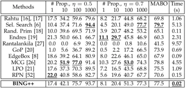
We first compare the performance of different BING’s derivatives on VOC2007 test dataset and COCO valida-tion dataset in Table 1, where the timing reported for all

the methods is based on multi-thread computation on our

server with two INTEL XEON E5 2696v2 [email protected].

3. In fact, BING can generalize to generic object proposals with-out training as shown in [51]. Here we follow the original BING implementation.

4. http://groups.inf.ed.ac.uk/calvin/objectness/. We downloaded the proposals using either NMS or multinomial sampling. In our experiments we observed that for top 1,000 proposals NMS works better than multinomial sampling. Therefore we only reported the performance using NMS.

5. https://github.com/batra-mlp-lab/object-proposals. We run the code for [15], [26], [17], [19], [18], [20], [21], [27], [6], [8].

6. http://www.cse.oulu.fi/CMV/Downloads/ObjectDetection/ 7. https://zimingzhang.wordpress.com/source-code/

8. https://github.com/varun-nagaraja/BING-Objectness 9. http://3dimage.ee.tsinghua.edu.cn/cxz/mtse 10. https://github.com/ShaoqingRen/faster_rcnn

TABLE 1

Performance comparison (%) among different BING’s derivatives.

MethodsDR, # Prop.,η= 0.5 DR, # Prop.,η= 0.7MABO Time 1 10 100 1000 1 10 100 1000 (1000) (ms) VOC2007 E-BING 20.234.1 65.8 91.3 10.819.9 42.8 63.7 72.5 1.7 S-BING 17.0 38.3 74.7 95.1 7.9 17.9 49.0 76.4 76.8 2.6 BING++ 17.442.1 75.7 93.7 8.1 20.4 51.3 77.3 77.5 2.9 MS COCO E-BING 5.5 10.3 27.8 56.1 2.7 5.6 15.2 31.5 50.1 2.1 S-BING 4.8 13.837.5 64.8 2.3 5.8 20.6 44.2 56.9 3.0 BING++ 4.8 14.837.2 62.6 2.3 6.4 21.2 43.1 56.0 3.7 TABLE 2

Effect of image resize operation on performance (%) in BING++.

MethodsDR, # Prop.,η= 0.5 DR, # Prop.,η= 0.7MABO Time 1 10 100 1000 1 10 100 1000 (1000) (ms) VOC2007 No+No 17.541.6 76.9 95.0 8.319.2 50.8 78.8 78.0 4.2 Yes+No 17.3 41.3 76.4 94.1 8.1 17.9 49.6 77.3 77.3 5.8 No+Yes 17.3 41.977.6 94.5 8.2 19.351.4 78.7 78.1 3.6 BING++ 17.442.175.7 93.7 8.120.451.3 77.3 77.5 2.9 MS COCO No+No 5.1 14.538.4 65.5 2.4 6.6 21.2 46.6 57.9 11.2 Yes+No 5.0 14.2 38.1 64.5 2.4 5.8 20.4 44.8 57.0 12.1 No+Yes 4.9 14.838.2 63.9 2.4 6.5 22.0 45.4 57.1 7.2 BING++ 4.8 14.837.2 62.6 2.3 6.4 21.2 43.1 56.0 3.7 We observe that: (1) In terms of proposal quality, BING++ works the best, and S-BING is better than E-BING. (2) In terms of computation, E-BING is more efficient than S-BING and BING++. To see the contribution of each component in Alg. 3 on the overall running time, we show the timing cost in percentage in Fig. 9. As we see, BING actually takes the largest portion of computation by 56.6%, segmentation is ranked as the second by 20.1%, and Alg. 2 for segmentation based refinement is ranked as the third by 16.0%. The extra computation for edge based refinement takes only 7.3%. The increase of timing in Table 1 roughly follows this distribution.

Fig. 9. Timing distribution

over components in BING++.

In BING++ image resize op-eration plays a very impor-tant role in reducing compu-tational time. To show its ef-fect on performance as well as running speed, we list all the comparison in Ta-ble 2, where “Yes/No” de-notes with/without resize

op-eration, the first “Yes/No” is for edge based refinement, and the second is for segmentation based refinement. In this context BING++ is equivalent to the “Yes+Yes” option. As we see here, all the four competitors perform similarly in terms of DR and MABO, especially when the number of proposals is small. This is because most of the objects with

low best overlap (BO) scores aresmallin terms of number

of pixels covered by the ground-truth bounding boxes, as shown in Fig. 7. Therefore, even ignoring small objects by resizing images has marginal effect on proposal quality for BING++, but results in significantly better computational efficiency.

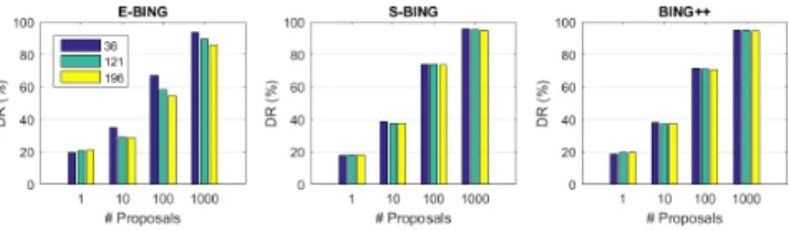
We also test the robustness of BING++ w.r.t. the quality

of BING proposals by varying the maximum number of

quantized scales/aspect-ratios (i.e.36, 121, 196) in BING to

generate different proposals (see the details in [4]). We then feed all these BING proposals into the three derivatives. We

Fig. 7. Distributions of objects based on their BO scores and the

width and height of their ground-truth bounding boxes, given the proposals from BING++ as inputs. For larger objects BING++ works better, in general.

Fig. 8. DR comparison on VOC2007 test dataset by varying the

maximum number of quantized scales/aspect-ratios in BING.

show the DR comparison in Fig. 8 (for MABO we observe similar behavior for each method). As we see E-BING (as well as BING) is actually sensitive to the parameter, but S-BING and BING++ are not. This is because segments are much stronger clues to estimate object boundaries than edges, leading to robust performance.

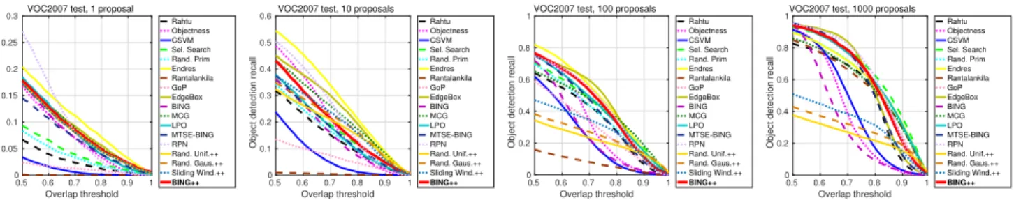
4.2 Benchmark Comparison (I): VOC2007

We first compare our BING++ with other proposal

algo-rithms using DRvs.IoU overlap threshold in Fig. 10. We also

implement three other baseline methods by replacing BING proposals in BING++ with bounding boxes sampled by (1) Random Uniform, (2) Random Gaussian, or (3) Sliding

Window11. These sampling methods have ignorable running

time, leading to faster speed than BING++, as shown in Table 3, yet much worse proposal quality. Overall, our BING++ behaves similarly to many other competitive pro-posal algorithms such as selective search, edgeBoxes, and GoP, especially when the number of proposals is sufficiently

large (e.g.100 or 1,000). Note that when the proposals are

sufficient, there are significant performance gaps between BING and our BING++, indicating that BING++ achieves huge improvement on DR over BING.

To quantify these plots, we list the corresponding

num-bers as well as the averagesingle-threadcomputational time

of each method in Table 3, which are called from MATLAB, except RPN. In both cases with IoU threshold equal to 0.5 or 0.7, BING++ can always achieve similar performance to the best ones. However, it is quite notable that BING++ is much faster than other competitive proposal algorithms. For instance, BING++ is 500 times faster than selective search.

11. We used the published code at https://github.com/hosang/ detection-proposals for [37] to sample 1,000 proposals.

0.5 0.6 0.7 0.8 0.9 1 Overlap threshold 0 0.05 0.1 0.15 0.2 0.25 0.3

Object detection recall

VOC2007 test, 1 proposal Rahtu Objectness CSVM Sel. Search Rand. Prim Endres Rantalankila GoP EdgeBox BING MCG LPO MTSE-BING RPN Rand. Unif.++ Rand. Gaus.++ Sliding Wind.++ BING++ 0.5 0.6 0.7 0.8 0.9 1 Overlap threshold 0 0.1 0.2 0.3 0.4 0.5 0.6

Object detection recall

VOC2007 test, 10 proposals

Rahtu Objectness CSVM Sel. Search Rand. Prim Endres Rantalankila GoP EdgeBox BING MCG LPO MTSE-BING RPN Rand. Unif.++ Rand. Gaus.++ Sliding Wind.++ BING++ 0.5 0.6 0.7 0.8 0.9 1 Overlap threshold 0 0.2 0.4 0.6 0.8 1

Object detection recall

VOC2007 test, 100 proposals Rahtu Objectness CSVM Sel. Search Rand. Prim Endres Rantalankila GoP EdgeBox BING MCG LPO MTSE-BING RPN Rand. Unif.++ Rand. Gaus.++ Sliding Wind.++ BING++ 0.5 0.6 0.7 0.8 0.9 1 Overlap threshold 0 0.2 0.4 0.6 0.8 1

Object detection recall

VOC2007 test, 1000 proposals Rahtu Objectness CSVM Sel. Search Rand. Prim Endres Rantalankila GoP EdgeBox BING MCG LPO MTSE-BING RPN Rand. Unif.++ Rand. Gaus.++ Sliding Wind.++ BING++

Fig. 10. Comparison of recall-overlap curves using different methods and numbers of proposals on VOC2007 test set.

TABLE 3

DR (%) and running time (s) comparison on VOC2007 test dataset.

Methods # Prop.,η= 0.5 # Prop.,η= 0.7 Time 1 10 100 1000 1 10 100 1000 (s) Rahtu [16], [17] 7.0 32.7 64.7 83.5 2.5 15.8 44.7 70.1 3.81 Objectness [15] 17.3 49.5 75.8 92.0 7.4 23.4 37.6 43.1 3.83 CSVM [4] 17.4 33.5 65.1 91.2 5.4 14.8 20.8 27.1 0.47 Sel. Search [6] 9.7 37.3 71.5 93.5 4.1 19.7 49.0 80.0 10.64 Rand. Prim [18] 8.6 35.0 70.4 90.3 3.5 17.3 45.1 73.4 0.79 Endres [19] 20.9 55.2 82.8 90.1 11.5 35.058.0 73.0 11.67 Rantalankila [27] 0.1 0.9 16.2 85.6 0.0 0.4 8.5 67.5 23.72 GoP [20] 2.4 13.8 60.2 94.2 1.3 7.7 35.1 77.8 1.26 EdgeBox [8] 17.8 45.8 75.4 95.1 9.5 30.960.8 85.1 0.25 BING [1] 18.2 37.3 73.0 95.2 7.3 16.9 24.5 29.1 0.01 MCG [26] 18.5 44.2 65.7 86.5 9.4 26.9 49.1 70.1 18.97 LPO [21] 18.5 38.0 75.5 94.4 8.0 18.0 49.2 76.8 1.43 MTSE-BING [9] 14.5 37.7 75.2 95.3 7.0 18.1 47.2 78.1 0.15 RPN [52] 27.1 50.3 74.8 95.2 8.0 27.8 54.9 82.4 0.14 Rand. Uniform++ 17.3 32.3 34.3 37.6 8.0 20.9 23.3 27.0 0.01 Rand. Gaussian++ 17.2 34.8 38.2 43.0 8.0 22.8 27.0 32.1 0.01 Sliding Window++ 17.2 37.4 47.0 50.8 8.0 23.6 34.6 38.4 0.01 BING++ 17.4 42.1 75.7 93.7 8.1 20.4 51.3 77.3 0.02 0 500 1000 # Proposals 0 0.2 0.4 0.6 0.8 1

Object detection recall

VOC2007 test set, IoU=0.5 Rahtu Objectness CSVM Sel. Search Rand. Prim Endres Rantalankila GoP EdgeBox BING MCG LPO MTSE-BING RPN Rand. Unif.++ Rand. Gaus.++ Sliding Wind.++ BING++ (a) 0 500 1000 # Proposals 0 0.1 0.2 0.3 0.4 0.5 0.6 0.7 0.8

Object detection recall

COCO validation, IoU=0.5

Sel. Search Rand. Prim Endres GoP EdgeBox BING MCG LPO MTSE-BING BING++ (b)

Fig. 11. Comparison of DRvs.number of proposals on VOC2007

test dataset(a)and MS COCO validation dataset(b), respectively.

Also by comparing BING++ with BING using IoU threshold equal to 0.7 and 1000 proposals, there is huge improvement again from 29.1% to 77.3%. This well demonstrates the capability of BING++ for generating high quality object proposals.

In order to understand the effect of image down-sampling on performance of different competitors, we resize the

images to either 1/3×1/3 = 1/9 of their original sizes

(used in edge-based refinement in BING++) or the fixed size

of360×400pixels (used in segmentation-based refinement

in BING++), respectively, and repeat the same experiments

in Table 3 and Table 4 using thedefaultparameters for each

algorithm without fine-tuning. The results are listed in Table 5 and Table 6, respectively. As we see: (1) Among the com-parison our BING++ is still the fastest as well as achieving comparable performance with the state-of-the-art. (2) The running time of RPN is quite similar in various experiments, because images are rescaled to the same size as inputs to the neural network. (3) For the rest of competitors, generally

speaking, the running time is improved, and the smaller the images are, the faster the methods can run. However, the DR and MABO become worse, in general. In Table 5 even if EdgeBox can run 4.5 times slower than BING++, its DRs are

12.8% (withη= 0.5and 1,000 proposals) and 12.3% (with

η= 0.7and 1,000 proposals) lower than those of BING++,

and its MABO is 9.6% lower than that of BING++.

Next we show the comparison of DR vs. number of

proposals in Fig. 11(a). Clearly with η = 0.5, BING++

performs among the top, which is consistent with Table 3. We also list our ABO and MABO comparison in Table 4. Still BING++ performs consistently close to the best performance among the competitors and finally achieves 77.5% MABO, only 3.9% smaller than selective search. As shown in [8], considering overall achievement this small difference is negligible in terms of proposal quality.

We also conduct the object detection task to measure the impact of DR, ABO and MABO of proposals on real applications, and list the results in Table 7. We run different algorithms to generate proposals and feed them to fast R-CNN [35] with pre-trained VGG-16 model [53] to perform detection. In terms of mean average precision (mAP), the overall detection performance of each competitive proposal

algorithm is quite close to each other,i.e. selective search,

GoP, EdgeBoxes, LPO, MTSE-BING, BING++ and its sib-lings. Also the average precision (AP) for each class from BING++ is close to the best performance among the com-petitors. We emphasize that the running time of BING++ is about 3ms per image only using CPUs on our server, which is much faster than any of the existing competitive proposal algorithms with good quality.

To better view the difference between different proposal algorithms for object detection, we illustrate some results in Fig. 12. Compared with BING, our BING++ produces more reasonable detections. Interestingly, the focuses of all the comparative algorithms are very similar even in such complex images, while the predicted bounding boxes vary.

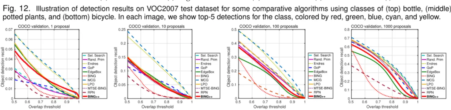
4.3 Benchmark Comparison (II): Microsoft COCO

Recall that on COCO for all the methods we keep using

the same (predefined or learned) parameters as those on

VOC2007 without any retraining. Because there are at least 60 different object classes between the two datasets, in such way we can compare the generalization ability of different methods for the purpose of generic object proposals across different object classes/datasets.

As on VOC2007, we first compare different algorithms

us-ing DRvs.IoU overlap threshold in Fig. 13. Due to the large

size of the dataset, here we only compare several relatively efficient algorithms. Again BING++ performs reasonably well among the top for all the cases. Interestingly EdgeBoxes

TABLE 4

ABO & MABO comparison (%) between different proposal algorithms on VOC2007 test dataset using 1,000 proposals.

Methods aer. bic. bird boat bot. bus car cat cha. cow din. dog hor. mot. per. pot. she. sofa tra. tv MABO Rahtu [17], [16] 72.6 74.5 69.0 69.7 49.0 79.9 67.2 82.6 62.9 72.9 80.5 80.6 78.5 74.5 65.7 58.9 69.8 82.3 79.5 73.8 72.2 Objectness [15] 67.3 69.0 65.6 64.4 57.1 72.3 65.3 72.8 64.8 67.6 73.3 71.1 70.9 67.6 63.5 61.4 65.6 74.7 70.6 65.5 67.5 CSVM [4] 70.4 70.2 67.6 66.7 58.9 73.6 67.6 76.5 64.9 68.0 74.1 74.7 72.7 71.4 66.6 62.3 67.9 75.6 74.5 66.7 69.6 Sel. Search [6] 83.5 83.1 80.1 78.1 62.8 85.2 77.7 90.7 77.0 83.2 88.6 89.4 82.9 81.9 72.6 71.2 80.4 90.3 85.7 83.7 81.4 Rand. Prim [18] 80.9 80.9 74.5 74.3 59.2 83.7 76.5 87.0 74.6 79.8 87.6 85.1 79.8 81.0 70.6 67.1 72.8 89.4 82.8 80.0 78.4 Endres [19] 71.0 81.0 72.3 65.5 60.9 85.1 79.1 87.9 72.4 80.3 87.0 87.1 82.2 82.9 70.5 67.4 76.2 89.7 84.5 79.1 78.1 Rantalankila [27] 73.5 74.6 73.5 66.7 54.0 81.3 72.7 89.2 68.6 76.4 83.2 87.4 81.0 76.0 66.2 62.8 72.1 87.1 82.0 77.5 75.3 GoP [20] 73.8 80.1 76.0 72.2 63.0 86.0 80.3 88.2 75.9 81.3 85.8 85.7 79.9 79.1 73.5 71.1 78.7 88.4 82.3 82.3 79.2 EdgeBoxes [8] 76.8 81.6 78.5 76.7 65.8 83.9 76.8 82.3 76.4 82.2 80.9 83.6 81.3 80.9 73.6 71.7 80.8 82.5 79.8 81.4 78.9 BING [1] 65.5 66.0 64.0 62.3 60.6 66.5 64.4 69.9 62.6 65.1 69.5 68.3 65.9 65.7 63.8 62.4 64.6 69.0 68.6 63.4 65.4 MCG [26] 75.2 77.3 73.3 68.9 55.3 81.4 70.8 87.5 69.6 80.5 82.8 86.0 78.8 75.6 67.9 61.3 78.7 88.7 81.2 76.2 75.9 LPO [21] 74.9 79.9 76.9 72.9 61.4 86.4 80.4 89.1 74.5 82.0 85.1 86.9 82.4 81.7 73.0 71.5 79.4 88.7 85.3 81.6 79.7 MTSE-BING [9] 78.7 77.6 75.5 75.3 63.3 80.6 75.3 83.2 75.8 78.5 82.7 81.9 77.3 78.1 72.1 71.1 76.9 84.0 77.7 79.9 77.3 RPN [52] 76.8 81.9 77.6 76.4 69.1 79.5 81.8 84.4 76.0 84.2 81.5 83.9 83.5 80.7 80.6 69.8 80.3 83.5 82.0 77.2 79.5 Rand. Uniform++ 56.7 42.2 35.5 37.0 11.1 51.5 35.8 64.5 22.6 30.8 57.3 59.0 54.1 46.5 29.6 21.1 25.1 59.2 58.3 24.2 41.1 Rand. Gaussian++ 59.2 47.2 39.1 41.2 13.1 56.5 39.1 68.9 26.4 34.8 63.4 64.3 60.4 51.3 33.8 24.3 29.3 64.6 62.7 28.1 45.4 Sliding Window++ 62.0 54.6 45.5 45.2 16.1 62.2 44.5 73.7 33.7 40.9 71.1 69.3 62.6 56.2 36.4 29.0 37.1 73.0 67.0 37.1 50.9 BING++ 79.5 78.5 76.6 75.2 60.0 81.5 75.5 85.3 72.4 78.2 83.6 84.0 79.7 79.2 70.7 68.7 77.9 85.5 79.8 77.2 77.5

(a) BING++ (b) BING (c) EdgeBoxes (d) LPO (e) MTSE-BING (f) Selective Search

Fig. 12. Illustration of detection results on VOC2007 test dataset for some comparative algorithms using classes of (top) bottle, (middle)

potted plants, and (bottom) bicycle. In each image, we show top-5 detections for the class, colored by red, green, blue, cyan, and yellow.

0.5 0.6 0.7 0.8 0.9 1 Overlap threshold 0 0.01 0.02 0.03 0.04 0.05 0.06 0.07

Object detection recall

COCO validation, 1 proposal

Sel. Search Rand. Prim Endres GoP EdgeBox BING MCG LPO MTSE-BING RPN BING++ 0.5 0.6 0.7 0.8 0.9 1 Overlap threshold 0 0.05 0.1 0.15 0.2 0.25

Object detection recall

COCO validation, 10 proposals

Sel. Search Rand. Prim Endres GoP EdgeBox BING MCG LPO MTSE-BING RPN BING++ 0.5 0.6 0.7 0.8 0.9 1 Overlap threshold 0 0.1 0.2 0.3 0.4 0.5

Object detection recall

COCO validation, 100 proposals

Sel. Search Rand. Prim Endres GoP EdgeBox BING MCG LPO MTSE-BING RPN BING++ 0.5 0.6 0.7 0.8 0.9 1 Overlap threshold 0 0.1 0.2 0.3 0.4 0.5 0.6 0.7 0.8

Object detection recall

COCO validation, 1000 proposals

Sel. Search Rand. Prim Endres GoP EdgeBox BING MCG LPO MTSE-BING RPN BING++

Fig. 13. Comparison of recall-overlap curves using different methods and numbers of proposals on MS COCO validation set.

seems to struggle on COCO. One possible reason is that images in COCO are more complex than those in VOC2007, in general, leading to noisy/missing edges which confuse EdgeBoxes. Another possible reason is that EdgeBoxes is quite sensitive to its parameters, and we need to re-tune its parameters using training data in COCO. Similarly the pre-trained RPN using VOC2007 data does not work well on COCO, indicating that the RPN method is not suitable for the purpose of generic object proposal generation as it is sensitive to the parameters. However, our BING++ is more robust to parameter settings. We list in Table 8 the corresponding numbers in Fig. 13 as well as MABO for nu-merical comparison. Note that compared with BING, both DR and MABO of BING++ are boosted significantly. Also

in Fig. 11(b) we show the behavior of different algorithms

using DRvs.number of proposals where BING++ performs

slightly worse. We speculate that this is because a large portion of small objects occurring in COCO worsen the performance, as we show in Fig. 7. Using 1,000 proposals

the BING++ performs inferiorly to the best (i.e.MCG), but

with about 1,000 times faster.

We also show the AP and mAP scores for object detection on COCO validation dataset in Fig. 14 using fast R-CNN with pre-trained VGG-16 model. Different from VOC2007, all the methods on AP in Fig. 14(a) behave similarly with marginal gaps. In terms of mAP shown in Fig. 14(b) BING++

performs comparably with the best method (i.e. selective