Kernel Support Tensor Regression

(1)

Procedia

Engineering

www.elsevier.com/locate/procedia

2012 International Workshop on Information and Electronics Engineering (IWIEE)

Kernel Support Tensor Regression

Chao GAO, Xiao-jun WU

*

School of IOT Engineering, Jiangnan University, Wuxi 214122, China

Abstract

Support vector machine (SVM) not only can be used for classification, can also be applied to regression problems by the introduction of an alternative loss function. Now most of the regress algorithms are based on vector as input, but in many real cases input samples are tensors, support tensor machine (STM) by Cai and He is a typical learning machine for second order tensors. In this paper, we propose an algorithm named kernel support tensor regression (KSTR) using tensors as input for function regression. In this algorithm, after mapping the each row of every original tensor or of every tensor converted from original vector into a high dimensional space, we can get associated points in a new high dimensional feature space, and then compute the regression function. We compare the results of KSTR with the traditional SVR algorithm, and find that KSTR is more effective according to the analysis of the experimental results.

Key words: Support Vector Machine(SVM); Support Vector Regression (SVR); Tensor; Support Tensor Machine (STM); kernel method; Kernel Support Tensor Regression (KSTM)

1. Introduction

The theory of SVM invented by Vapnik is a popular machine learning method based on the statistical learning theory [1-3]. It can be used for classification and regression. It is called support vector regression (SVR), when it is used for function regression [4]. SVR has been successfully used in a lot of practical field. In 2005, support tensor machine was proposed by Cai and He [5], it used tensor as input for classification. It is only a linear method, it difficult to deal with nonlinear data. In this paper we extend STM and kernel method [6,7] to tensor data for regression. We propose a kernel function for tensor. Using

*Corresponding author. Tel.: +86 510 8591 3612.

E-mail address: [email protected].

Open access under CC BY-NC-ND license.

(2)

the function we can map the tensor sample into a high dimensional tensor feature space, then search a couple of parallel hyperplanes, making all the training samples between the hyperplanes.

The rest of this paper is organized as follows. In section 2 we introduce the kernel function for tensors. In section 3 we derive the KSTR algorithm. The experimental results on 6 data sets are shown in section 4. Finally, in section 5 we draw conclusions of our paper.

2. The Kernel Function for Tensors

Suppose we are given a set of training samples

{

X y i

_i

,

_i

}

,

=

1, 2,...

m

, each of the training sample

X

_i

is a data point in

R

n1

⊗

R

n2_{, where}

R

n1_and

R

n2 _{are two vector spaces, and}

i

y

is the target value

associated with

X

_i. Take

z

_ip as the p-th row of

X

_i, and then use a nonlinear mapping function

ϕ

( )

X

_i

to map

X

_i into a high dimensional tensor feature space, so we can define a nonlinear mapping function

for tensor

X

_i: 1 1 2

( )

(

( )

)

i i i in

z

X

z

ϕ

⎡

⎤

⎢

⎥

⎢

⎥

Φ

= ⎢

⎥

⎢

⎥

⎢

⎥

⎣

⎦

M

(1)

We can get the new kernel function:

(

)

( )

1 1 1 1 1 1 1 1 1 1 1 2 2 1 ( ) ( ) ( ) ( ) ( ) ( ) ( ) ( ) , ( ) ( ) ( ) ( ) ( ) ( ) j T T i i j in jn T _i _j i j i j T T in j in jn in jn T z z z z z z z z K X X X X z z z z z z ϕ ϕ _ϕ _ϕ _ϕ _ϕ ϕ ϕ ϕ ϕ ϕ ϕ ϕ ϕ ⎡ ⎤ ⎡ ⎤ _⎛ _⎞ ⎢ ⎥ ⎢ ⎥ _⎜ _⎟ ⎢ ⎥ ⎢ ⎥ =_⎢ _⎥_⎢ _⎥ = ⎜ ⎟ ⎜ ⎟ ⎢ ⎥ ⎢ ⎥ _⎝ _⎠ ⎢ ⎥ ⎢ ⎥ ⎣ ⎦ = Φ Φ ⎣ ⎦ K M O M L M M (2)

( )

X

_i

Φ

and

K X X

(

i

,

j

)

will be used in the following parts.

This kernel function is different from the function of SVR: the result of STR is a matrix while that of SVR is a scalar. For instance, in KSTR method if we use RBF kernel function, then the ij-th element of the kernel matrix is

( ) ( )

2 1 2 1 2 ip jp T z z ip jp

z

e

γ

ϕ

− −

=

(3)

3. Support Tensor Regression with

ε

-insensitive Loss Function

Support Tensor regression with

ε

-insensitive Loss Function is similar with support tensor regression.

Suppose we are given a set of training samples

{

X y

_i

,

_i

}

,

i

=

1, 2,...

m

, each of the training sample

X

_i is

a data point in

R

n1

⊗

R

n2 _{, where}

R

n1_and

R

n2 _{are two vector spaces, and}

i

y

is the target value

associated with

X

_i. The regression function we want to get is:

( )

T

( )

f X

=

u

Φ

X v b

+

(4) The function can be given by the following optimal quadratic programming problem:

(3)

* 2 _* , , , , ₁ * *

1

Minimize

(

)

2

S.T.

,

1,

( )

, ,

,

2

0

i i m T i i u v b _i i i i i i T i i T i

u

X

uv

v b

u

X v

C

y

i

m

y

b

ξ ξ

ε ξ

ξ ξ

=

+

⎧

−

⎪

=

…

+

⎨

⎪

≥

⎩

+

− Φ

− ≤

Φ

+ − ≤

∑

：

(5)

where

C

is a pre-specified value,

ε

is a scalar defined by ourselves, and

ξ ξ

_i

,

_i* are slack variables representing upper and lower constraints on the outputs of the system.

1. Let

u

be a column vector whose dimension is the same as the row number of samples.

2. Calculate

v

. Using lagrangian multiplier method to construct the lagrangian according to (5):

(

)

( )

(

)

(

( )

)

* * * 2 _* _{* *} 1 1 * * 1 1 , , , , , , * * . . , , , 0, 1, 2,... 2 , 1 ₍ ₎ i i i i i i m m T i i i i i i i i m m T T i i i i i i i i i i v b i i i i uv C y u L Max Min S T i m X v b y u X v b ξ ξ α α η η

α α η η

ξ ξ

η ξ η ξ

α ε ξ

= = = = + − + − + − + Φ ⎧ ⎫ = + ⎪ ⎪ ⎪ ⎪ ⎨ ⎬ ⎪ ⎪ ⎪ + − + − + Φ + ⎪ ⎩ ⎭ ≥ =

∑

(6)

where

α α η η

_i

,

_i*

, ,

_i _i* are lagrangian multipliers.

Solving (6) determines the lagrangian multipliers

α α

_i

,

_i*. Then we can get

v

and

v

2. 3. Calculate

u b

,

.According to the result of the first part, we can let

( )

(

) (

)

'' * 4 1

,

1

m T T j j i i j i i

x

v

X

K X

u

=

α α

X

= Φ

=

∑

−

(7)

as the new training samples. According to (5), we can construct another lagrangian:

(

)

(

)

(

)

* * * 2 _* _{* *} 1 1 '' * * ' , , , , 1 , 1 , * ' *

. .

,

, ,

0,

1, 2

1

(

)

,...,

2

i i i i i i m m T i i i i i i i i m m i i i i u b i i i i i i i i i i

uv

C

y

x u b

y

x u

L

Max Min

S T

i

m

b

α α η η ξ ξ

ξ ξ

η ξ η ξ

α

η

ξ

α

ξ

α

η

ε

= = = =

⎧

⎫

=

+

⎪

⎨

⎬

⎪

+

−

+

−

+ − +

+ −

+

+ −

− ⎪

⎪

⎩

⎭

≥

=

∑

(8)

where

α α η η

_i

,

_i*

, ,

_i _i* are lagrangian multipliers.

Solving (8) determines the lagrangian multipliers, then we can get

u

and

b

.

4. Iteration. Using step 2 and step 3, we can iteratively compute

v u b

, ,

.

4. Experiments and Analysis

In order to validate the performance of our algorithm, we evaluated our KSTR method using 6 data sets. These data sets are SIN, HOUSING, MPG, ABALONE, PYRIM, BODYFAT respectively. In order to

achieve good generalization performance, we have used 15 different values of kernel parameter

γ

and

(4)

100, 1000, 10000. The 15 different values of

C

are chosen as 0.001, 0.01, 0.05, 0.1, 0.2, 0.5, 1, 2, 5, 10, 20, 50, 100, 1000, 10000. Generally, the samples are vectors we convert them into second order tensors at first. When the product of row and column is less than the dimension of original vector, we would fill with constant 1 into the tensor.

Table 1. Feature of the data sets

Number of training samples

Attribute The size of converted tensor Numbers of training samples sin 200 1 1*1 20,30,40,50,60 HOUSING 506 13 4*4 20,30,40,50,60 MPG 392 7 2*4 20,30,40,50,60 ABALONE 4177 8 2*4 20,30,40,50,60 Pyrim 74 27 3*9 20,30,40,50,60 bodyfat 252 14 2*7 20,30,40,50,60

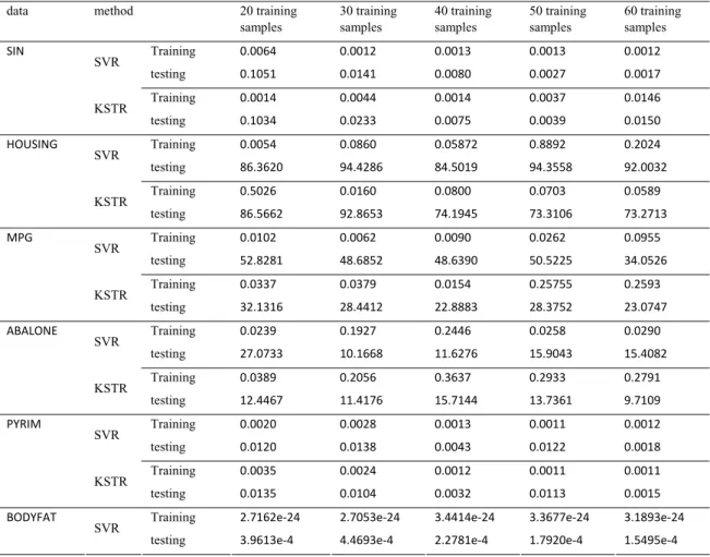
Table 2. The mean square error of regression

data method 20 training

samples 30 training samples 40 training samples 50 training samples 60 training samples Training 0.0064 0.0012 0.0013 0.0013 0.0012 SVR testing 0.1051 0.0141 0.0080 0.0027 0.0017 Training 0.0014 0.0044 0.0014 0.0037 0.0146 SIN KSTR testing 0.1034 0.0233 0.0075 0.0039 0.0150 Training 0.0054 0.0860 0.05872 0.8892 0.2024 SVR testing 86.3620 94.4286 84.5019 94.3558 92.0032 Training 0.5026 0.0160 0.0800 0.0703 0.0589 HOUSING KSTR testing 86.5662 92.8653 74.1945 73.3106 73.2713 Training 0.0102 0.0062 0.0090 0.0262 0.0955 SVR testing 52.8281 48.6852 48.6390 50.5225 34.0526 Training 0.0337 0.0379 0.0154 0.25755 0.2593 MPG KSTR testing 32.1316 28.4412 22.8883 28.3752 23.0747 Training 0.0239 0.1927 0.2446 0.0258 0.0290 SVR testing 27.0733 10.1668 11.6276 15.9043 15.4082 Training 0.0389 0.2056 0.3637 0.2933 0.2791 ABALONE KSTR testing 12.4467 11.4176 15.7144 13.7361 9.7109 Training 0.0020 0.0028 0.0013 0.0011 0.0012 SVR testing 0.0120 0.0138 0.0043 0.0122 0.0018 Training 0.0035 0.0024 0.0012 0.0011 0.0011 PYRIM KSTR testing 0.0135 0.0104 0.0032 0.0113 0.0015

Training 2.7162e‐24 2.7053e‐24 3.4414e‐24 3.3677e‐24 3.1893e‐24 BODYFAT

SVR

(5)

Training 1.4028e‐8 5.5008e‐8 3.6980e‐8 3.7530e‐8 4.7533e‐8

KSTR

testing 3.9589e‐4 2.5805e‐4 1.3265e‐5 8.4.38e‐5 2.1490e‐4

In every experiment training data are randomly selected from the data sets, and results are the average mean square error obtained after 10 random selections of training samples. Table 2 shows the experience results of training data and test data. The mean square errors of training samples are almost as same as traditional SVR method; and most of the mean square errors of testing samples using KSTR method are better than SVR method. So the predicted results are much more approximate to the target values. It means that the generalization ability of KSTR method is superior to that of traditional SVR method. Therefore, the regression performance of KSTR method is significantly better than that of traditional SVR.

5. Conclusion

In this paper we develop a regression method named kernel support tensor regression (KSTR) which is improved from support vector regression (SVR). For one thing, it uses tensors for inputs, so that we can get more information from the training samples; for another, a new kernel function was proposed for tensor, therefor, it also can solve nonlinear problems. KSTR can use all the kernel functions of SVR. According to the experiments we can see KSTR has better performance than traditional SVR. The experimental results show that mean square errors of KSTR method with testing samples are small than that of SVR method. And the regression ability of KSTR method is better than SVR method. The KSTR method has most of the advantages of SVR method: it has strong ability of learning and superior generalization ability. The kernel method makes KSTR solving nonlinear separable problems easily. A disadvantage of KSTR is that the computational load of KSTR is much bigger than that of SVR.

Acknowledgements

This work was supported in part by the following projects: Program for New Century Excellent Talents in University of China (Grant No.: NCET-06-0487), National Natural Science Foundation of P. R. China (Grant No.: 60973094), and Fundamental Research Funds for the Central Universities (Grant No. JUSRP31103).

References

[1]Vapnik V N. The Nature of Statistical Learning Theory. New York: Springer-Verlag, 1995. [2]Vapnik V N.Statistical Learning Theory. Wiley, NY, 1998.

[3] Chong Jin Ong, Shi Yun Shao. An Improved Algorithm for the Solution of the Regularization Path of Support Vector Machine, Transactions on Neural Networks, January, 2009

[4] Li-Tang Qian, Shu-Shen Liu. Support vector regression and least squares support vector regression for hormetic dose-response curves fitting, Chemosphere, Volume 78, Issue 3, January 2010, Pages 327-334.

[5] Deng Cai, Xiaofei He, Jiawei Han. Learning with Tensor Representation.Department of Computer Science Technical Report No. 2716, University of Illinois at Urbana-Champaign (UIUCDCS-R-2006-2716).April 2006.

[6]NelloCristianini, John Shawe-Taylor. An Introduction to Support Vector Machines and Other Kernel-based Learning Methods. Cambridge University Press,2000.

Open access under CC BY-NC-ND license