June 2000
Submitted to ICONIP 2000
ENVIRONMENTAL DATA MAPPING
WITH SUPPORT VECTOR REGRESSION
AND GEOSTATISTICS
Mikhail Kanevski
Patrick Wong
1Stephane Canu
2IDIAP-RR-00-10
1 University of New South Wales, Sydney, NSW 2052, Australia, 2 INSA; Place Emile Blondel, 76131 Mont-Saint-Aignan, France
Environmental Data Mapping with
Suppo rt Vector Regression and Geostatistics
M. KanevskiIDIAP – Dalle Molle Institute of Perceptual Artificial Intelligence CP 592, 1920 Martigny, Switzerland
P.M. Wong Petroleum Engineering U. of New South Wales Sydney, NSW 2052, Australia
S. Canu
Institut National des Sciences Appliquées Place Emile Blondel, B.P. 08 76131 Mont-Saint-Aignan Cédex, France
Abstract
The paper presents decision-oriented mapping of pollution using hybrid models based on statistical learning theory (support vector regression or SVR) and spatial statistics (geostatistics). Adaptive and robust SVR approach is used to model non-linear large scale trends in the region and geostatistical models – spatial predictions and spatial simulations – are used to prepare decision-oriented maps: prediction maps along with maps of error variance and equiprobable digital models of the pollution based on conditional stochastic simulations. The quality of the proposed approach is tested with the validation data set not used for the model development. Real data on soil contamination by Chernobyl radionuclides in Russia is used as a case study.
1. Introduction
In this paper, the ideas of hybrid models based on machine learning (data-driven) approach and geostatistics firstly presented in (Kanevski et al., 1996) are developed using recent developments in statistical learning theory (Vapnik, 1998) – support vector regression – and geostatistics. The model is applied to real data on soil contamination by Chernobyl radionuclides in the most contaminated region of Russia (Briansk region). Exploratory data analysis and especially exploratory variography and variogram modelling are widely used for better understanding of data and the results.
2. Support Vector Regression
The first publication on the adaptation of support vector regression (SVR) to spatial data can be found at Kanevski and Canu (2000). Detailed explanations on SVM can be found in a number of recent publications (e.g. Christianini and Shave-Taylor, 2000). In the present paper only basic equations are presented.
Let us assuming f is a prediction function (i.e. a function used to predict the value of Z knowing the geographical co-ordinates (x,y). We define the cost of choosing this particular function for a given decision process. First, for a given observation (x,y,Z), we define the ε-insensitive cost function:
− − − > = otherwise 0 | ) , ( | if | ) , ( | } , , ), , {(x y Z ε f f x y Z ε f x y Z ε C
where ε characterizes some acceptable error.
Now, for all possible observations, we define the global or generalisation error also known as the integrated prediction error IPE:
dxdy y x f Z y x C E f IPE Z( (( , ,) , , )) ( , ) ) ( =
∫
ε ωwhere ω(x,y) is some economical measure, indicating the relative importance of a mistake at point (x,y). Usually
ω(x,y) = 1, so that all positions are assumed to be equally important.
Now we are going to define where to look for the solution of the problem of minimising the integrated prediction error: 0 1 ) , ( ) , (
∑
ϕ ω = ∧ + = m k k k x y w y x fThe complexity of the solution can be tuned through
∑
= = m k k w w 1 2 2(Vapnik, 1998). Thus, a relevant strategy to minimise IPE is to minimise the empirical error together with maintaining w2small. This can be obtained by minimising the following cost function:
≤ i= ,...n y x f w i i i, )-Z | ,for 1 , ( | subject to || || 2 1 minimize i 2 ε
But, unfortunately, some data may lie outside of this epsilon tube due to noise or outliers making these constraints too strong and impossible to fulfil. In this case Vapnik suggests to introduce so called slack variables
) ,
(ξi ξi* . These variables measure the distance between the
observation and the
ε
and (ξi,ξi*) is illustrated by thefollowing example: imagine you have a great confidence in your measurement process, but the variance of the measured phenomena is large. In this case,
ε
has to be chosen a priori very small while the slack variables) ,
(ξi ξi* are optimised and thus can be large. Remember
that inside the epsilon tube
[
f( )
x,y −ε,f( )
x,y +ε]
cost function is zero.Note that by introducing the couple (ξi,ξi*) the
problem has now 2n unknown variables. But these variables are linked since one of the two values is necessary equals to zero. Either the slack is positive
) 0 (ξi*=
or negative
(ξi =0). Thus:
( )
( )
[
*]
, , , i i i f x y f x y Z ∈ −ε−ξ +ε+ξNow, we are looking for a solution minimising at the same time its complexity (measured by w2) and its prediction error (represented by max (ξi,ξi*)=ξi+ξi*). In
this case, let us introduce a user specified trade off parameter C between these two contradictory objectives. That leads us to the following problem:
∑
= + + n i i i C 1 * 2 ) ( || || 2 1 minimise ω ξ ξ ≥ ≤ − + − ≤ − − ,...,n = i Z y x f Z y x f i i i i i i i i i i i 1 for 0 , ) , ( ) , ( subject to * * ξ ξ ξ ε ξ εA classical way to reformulate a constraint based minimisation problem is to look for the saddle point of Lagrangian L:
∑
∑
∑
∑
= = = = + − + + − − + + − − + + = n i n i i i i i i i i i i i n i n i i i i i i i i i Z y x f y x f Z C w w L 1 1 * * * * 1 1 * 2 * ) ( ) ) , ( ( ) ) , ( ( ) ( || || 2 1 ) , , ( ξ η ξ η ξ ε α ξ ε α ξ ξ α ξ ξwhere αi,αi*,ηi,ηi* are Lagrangian multipliers associated
with the constraints. They can be roughly interpreted as a measure of the influence of the constraints in the solution. A solution with αi =αi*=0 can be interpreted as “the
corresponding data point has no influence on this solution”. At the minimum the derivative of the Lagrangian equals to zero (Kuhn-Tacker conditions):
n 1,..., = i for n 1,..., = i for 1,...m = k for ) , ( ) ( * * 1 * i i i i n i i i k i i k C C y x w α η α η ϕ α α − = − = − =
∑
=These variables can be removed from the original formulation of the minimisation problem to get the dual formulation of the problem:
= ≤ ≤ = − − + + − − −
∑
∑
∑
∑∑
∑
= = = = = ,..., 1 for , 0 , 1 for 0 ) , ( ) ( subject to ) ( ) ( ) ( ) , ( ) , ( ) ( 2 1 maximise * n 1 = i * 1 1 * * 1 1 * 1 * n i C m ,... = K y x K Z y x y x i i j i i j i i n i n i i i i i i i n i n j j j m k j j k i i k i i α α α α α α α α ε α α ϕ ϕ α αThis problem is untractable because of functions
ϕ
. Now we are going to solve the optimization problem without specifying functionsϕ
k. To do so it is necessary tochoose
ϕ
k such that:(
( , ),( , ))
) , ( ) , ( 1 j j i i j j k i i m k k x y x y =G x y x y∑
= ϕ ϕThis is the case in reproducing kernel Hilbert space, where G is the reproducing kernel. Functions
ϕ
k are theeigen functions of G. In this case the solution can be formulated in the following form:
∑
= ∧ + = n i i i iG x y x y b v y x f 1 )) , ( ), , (( ) , (with vi =(α −i* αi). Note that function
ϕ
k hasdisappeared. This solution only depends on the kernel function G. Note also that here at least one of alphas is equalled to zero depending of the observed value Zi, above
or under the
ε
-tube.The main difficulty of this QP problem lies in its dimension. For 1000 data points the problem to be solved is of dimension 2000 that makes it intractable for most of the commercial optimisation software. Equality constraints are not too complex since they are very few. Box constraints are also rather simple but there are many of them (4n). This suggests to use a specific algorithm taking into account the specificity of the box constraints.
A typical practical choice for the kernel is the Gaussian Kernel: 2 2 2 ) ( ) ( exp )) , ( ), , (( σ j i j i j j i i y y x x y x y x G = − − + −
where
σ
denotes the bandwidth of the kernel.The hyperparameters of the SVR can be tuned using splitting of the original data into training, testing and validation sets.
3. Ordinary Kriging
Details on the geostatistical spatial predictions can be found in a number of recent books (e.g. Goovaerts, 1997; Deutsch and Journel, 1997). In the present study, so-called ordinary kriging model (valid under the hypotheses of second order stationarity and intrinsic random function) is used for the spatial predictions of the residuals.
4. Case study
Case study is based on a real data on soil contamination by Chernobyl radionuclides. Data demonstrates variability at several spatial scales (spatially non-stationary data). In this case traditional geostatistical models based on a hypothesis of second order stationarity or intrinsic hypothesis can not be used directly. In the present research hybrid models based on SVR adaptive modeling of large scale trends and analysis and modeling of the residuals with geostatistical model (ordinary kriging) is applied. The approach follows the ideas presented in (Kanevski et al., 1996) where artificial neural networks were used for the large scale de-trending. The SVRRK/SVRRSIMM – Support Vector Regression Residual Kriging/Support Vector Regression Residual Simulations - models follow the ideas of the NNRK approach and consist of several main phases:
• Exploratory data analysis,
• Trend analysis,
• Exploratory variography and modeling,
Semivariogram/variogram is the basic tool of the spatial structural analysis and variography. Theoretical formula (under the intrinsic hypotheses, Deutsch and Journel 1997)
Empirical estimate of the variogram (experimental variogram) is following
here N(h) – is a number of pairs separated b y a vector
h.
• SVR trend modeling (de-trending),
• Comprehensive analysis of the residuals,
• Exploratory variography and modelling of the residuals,
• Validation of the results and final predictions.
The main outputs of the SVRRK model are presented below.
SVR detrending
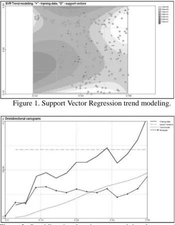
Let us present the results of large scale modelling using Support Vector Regression approach. In order to model large scale trend in the region, kernel bandwidth of the SVR was selected equal to the scale of the region. The results are presented in Figure 1.
Figure 1. Support Vector Regression trend modeling.
Figure 2. Omnidirectional variograms: training data, trend model, SVR residuals.
The general spatial correlation structures can be understood from the omnidirectional variograms, presented in Figure 2. Raw training data represent variability at different scales. Variogram of trend model represents smooth function behaviour, and the variogram of the residuals represents small scale variability (second order stationary random function).
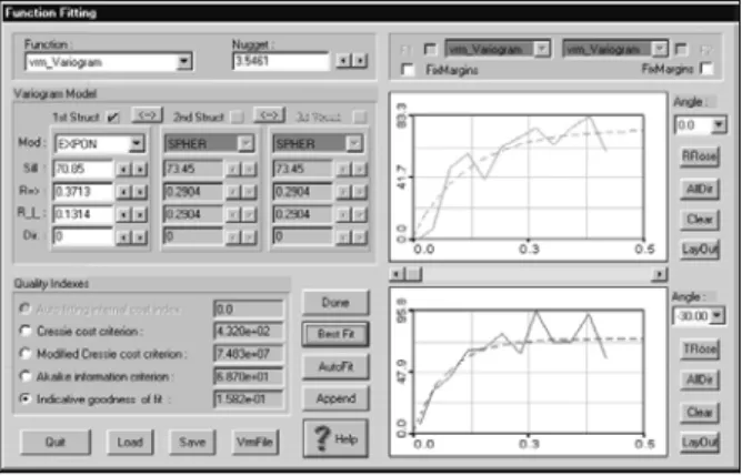
Geostatistical modeling of the residuals
In order to use geostatistical models – anisotropic
{
} (
{
)
}
γ
( , )
x h
=
1( )
x
− + =
(
x h
)
( )
x
− +
(
x h
)
=
γ
( )
h
2 2Var Z
Z
E Z
Z
(
)
γ
( ) ( ) ( ) ( ) ( ) h h x x h h = − + =∑
1 2 2 1 N i Zi Zi Nmeasures of spatial continuity (variograms) have to be analyzed and modeled (Goovaerts ). Directional variogram modeling of the residuals using Geostat Office software (Kanevski et al 1999b) is presented in Figure 2.
Prediction mapping with SVRRK model
The results of the Support Vector Machine Residual Kriging Model consist of trend modeling with SVR and residual predictions with ordinary kriging. The results of the residuals modeling with ordinary kriging are presented in Figure 3.
Figure 3. Variogram modelling of the SVR residuals.
Figure 4. Mapping of SVR residuals. Small scale structures can be recognized.
The main result is presented in Figure 4. Let us remind that SVRRK model is an exact model: at the measurement points outputs of the model equals to the measurement data.
Figure 5. Support Vector Regression residual Kriging Model Mapping.
Validation of SVRRK model
The model was used to predict independent (not used for training and tuning of the parameters) validation data set. The results are presented in Figure 7.
Figure 6. Validation of the SVRRK model with independent validation data set.
Support Vector Regression Residuals Simulation Model
All regression models, by definition, give some averages of data and do not represent spatial variability and uncertainty. Usually, reproducing of variability is a target of simulation models. In case of spatial data there have been developed several approaches and models for the conditional (to the original data) spatial simulations preserving basic spatial statistical characteristics: histograms of declustered data, variograms (see details in Goovaerts 1997): sequential gaussian simulations, indicator simulations, simulated annealing, etc. Most of the simulation models are based on so-called second order stationary random functions, when conditional mean value in the region is constant and spatial covariance function depends only on the separation vector between points.
One of the possibility how to avoid problems of second order stationarity is based on the same ideas as SVRRK model. Trends (large scale structures) are modeled with SVR and spatially correlated residuals are
used for simulations.
Simulations differs from any interpolation model. There are two major differences between estimations and simulations:
• The main objectives of the interpolators are to provide “best” local estimates z*(u) of each unsampled value z(u) without specific regard to the resulting spatial statistics of the estimates. In case of simulations the resulting global features and statistics (the same first two experimentally found moments - mean and covariance or variogram, as well as the histogram) of the simulated values take precedence over local accuracy. Stochastic simulation is a process of preparing alternative, equally probable, high resolution models of the spatial distribution of z(u). The variable can be categorical, indicating presence or absence of a particular characteristic, or it can be continuous.
• Kriging, for example, provides a single numerical model, which is the “best” in some local sense. Simulations provide many alternative numerical models zl(u), each of which is a “good” representation of the reality in some global sense. The difference between these alternative models or realizations provides a measure of joint spatial uncertainty.
In general, the objectives of simulation and estimation are not compatible. Simulations reproduce spatial variability and can take into account different sources of information (data integration).
In the present paper sequential gaussian simulations are considered. Gaussian random function models are widely used in statistics and simulations due to their analytical simplicity, they are well understood, they are a limit distributions of many theoretical results and were successfully applied in many cases. In this work we shall use algorithm known as a Sequential Gaussian Simulations.
Sequential Gaussian simulation methodology consists of several steps:
1. Determine the univariate cdf (cumulative distribution function) FZ(z) representative of the entire study area
and not only of the z-sample data available. Declustering may be needed.
2. Using the cdf FZ(z), perform the normal score
transform of z-data into y-data with a standard normal cdf.
3. Check for bivariaty normality of the normal score y-data.
4. If a multivariate Gaussian normality random function model can be adopted for the y-variable, local conditional distribution is normal with mean and variance obtained by simple kriging. The stationarity requires that simple kriging (SK) with zero mean should be used. If there are enough conditioning data to consider inference of a
non-stationary random function model it is possible to use mowing window estimations with ordinary kriging (OK) with the re-estimation of the mean. But in any case SK variance should be used for the variance of the Gaussian conditional cumulative distribution function if there are enough conditioning data it might be possible to keep the trend as it is.
5. Start with sequential Gaussian simulations:
• Define a random path, that visits each node of the grid (not necessarily regular) once. At each node u, retain a specified number of neighboring conditioning data including both original y-data and previously simulated grid node y-values.
• Use simple kriging with the normal score variogram model to determine the parameters (mean and variance) of the ccdf (conditional cumulative distribution function) of the random function Y(u) at location u.
• Draw a simulated value yl(u) from that ccdf.
• Add the simulated value yl(u) to the data set.
• Proceed to the next node, and loop until all nodes are simulated.
6. Back transform the simulated normal values yl(u) into simulated values for the original variable zl(u).
An important phase of sequential gaussian simulations deals with variography of normal score values (transformation form original data to univariate gaussian distribution N(0,1).
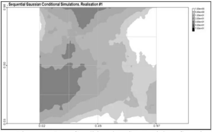
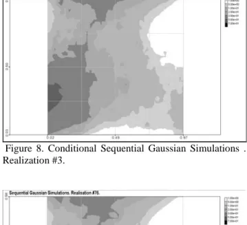
Some results of the sequential gaussian conditional simulations are presented in Figures 7-9. These figures are much variable in space.
The similarity and dissimilarity between digital models of the reality describes spatial variability and uncertainty. The next step deals with the probabilistic mapping: mapping to be Above some predefined decision level. This is a topic of another research related to decision oriented mapping of contaminated territories.
Figure 7. Conditional Sequential Gaussian Simulations. Realization #1.
Figure 8. Conditional Sequential Gaussian Simulations . Realization #3.
Figure 9. Conditional Sequential Gaussian Simulations. Realization # 76.
Usually hundreds of simulated models (realizations) are generated. The similarity and dissimilarity between different equiprobable realizations of the reality (using data and available knowledge) describes spatial variability and uncertainty of data. By developing many of equiprobable realizations probabilistic/risk mapping is possible as well: mapping of probability to be above/below some predefined decision/regulation levels. Detailed description of SVRRSim models and their application to the decision oriented mapping is under study and will be published elsewhere.
5. Conclusion
The results of spatial data mapping with hybrid model SVRRK are promising. Application of Support Vector Regression data driven and robust approach allowed to develop non-linear large scale model (trend model) in the region under study. The remaining residuals describing small scale variability of pollution were efficiently modelled using ordinary kriging model of geostatistics. There is a mutual relationship between models in SVRRK:
from one side geostatistical approach help to understand how much spatially structured information described by variograms was extracted from data by SVR, and from another side SVR can be used as an efficient tool for spatial data detrending in case of spatially non stationary data. Application of the conditional stochastic simulation models for the SVR residuals is under study.
The results of conditional simulations seems to be promising. After SVR detrending nscore transformation of the residuals demonstrates that second order stationary model can be accepted.
In conclusion, when working with spatially distributed data, self-consistent hybrid models using machine learning algorithms and geostatistics can bring mutual benefit for the both data driven and model dependent approaches. Acknowledgments
The research was supported in part by European INTAS grants 31726 and 99-00099.
References
Deutsch C.V. and A.G. Journel. GSLIB: Geostatistical Software Library and User’s Guide. Oxford University Press, New York, 1997.
Goovaerts P. Geostatistics for Natural Resources Evaluation. Oxford University Press, New York, 1997. Kanevski M., Arutyunyan R., Bolshov L., Demyanov V., Maignan M. Artificial neural networks and spatial estimations of Chernobyl fallout. Geoinformatics. Vol.7, No.1-2, 1996, pp.5-11.
Kanevski M., N. Gilardi, M. Maignan, E. Mayoraz. Environmental Spatial Data Classification with Support Vector Machines. IDIAP Research Report. IDIAP-RR-99-07, 24 p., 1999a. (www.idiap.ch)
Kanevski M, V. Demyanov, S. Chernov, E. Savelieva, A. Serov, V. Timonin, M. Maignan. Geostat Office for Environmental and Pollution Spatial Data Analysis. Mathematische Geologie, N3, April 1999b, pp. 73-83. Kanevski M., S. Canu. Environmental and Pollution Data Mapping with Support Vector Regression. IDIAP Research Report RR-09-00. www.idiap.ch
Smola A.J., and B. Scholkopf. A Tutorial on Support Vector Regression. NeuroColt2 technical Reports Series, NC2-TR-1998-030, October 1998.
Vapnik V. Statistical Learning Theory. John Wiley & Sons, 1998.