Fei, Weiyin and Hu, Liangjian and Mao, Xuerong and Shen, Mingxuan
(2018) Structured robust stability and boundedness of nonlinear hybrid
delay systems. SIAM Journal on Control and Optimization. ISSN
0363-0129 (In Press) ,
This version is available at https://strathprints.strath.ac.uk/64134/
Strathprints is designed to allow users to access the research output of the University of Strathclyde. Unless otherwise explicitly stated on the manuscript, Copyright © and Moral Rights for the papers on this site are retained by the individual authors and/or other copyright owners. Please check the manuscript for details of any other licences that may have been applied. You may not engage in further distribution of the material for any profitmaking activities or any commercial gain. You may freely distribute both the url (https://strathprints.strath.ac.uk/) and the content of this paper for research or private study, educational, or not-for-profit purposes without prior permission or charge.
Any correspondence concerning this service should be sent to the Strathprints administrator:
The Strathprints institutional repository (https://strathprints.strath.ac.uk) is a digital archive of University of Strathclyde research outputs. It has been developed to disseminate open access research outputs, expose data about those outputs, and enable the
Structured Robust Stability and Boundedness of
Nonlinear Hybrid Delay Systems
Weiyin Fei
1, Liangjian Hu
2,∗, Xuerong Mao
3, Mingxuan Shen
1,41
School of Mathematics and Physics,
Anhui Polytechnic University, Wuhu, Anhui 241000, China.
2
Department of Applied Mathematics,
Donghua Univerisity, Shanghai 201620, China.
3
Department of Mathematics and Statistics,
University of Strathclyde, Glasgow G1 1XH, U.K.
4
School of Science, Nanjing University of Science and Technology,
Nanjing, Jiangsu 210094, China.
Abstract
Taking different structures in different modes into account, the paper has devel-oped a new theory on the structured robust stability and boundedness for nonlinear hybrid stochastic differential delay equations (SDDEs) without the linear growth condition. A new Lyapunov function is designed in order to deal with the effects of different structures as well as those of different parameters within the same modes. Moreover, a lot of effort is put into showing the almost sure asymptotic stability in the absence of the linear growth condition.
Key words: Hybrid SDDEs, robust stability, robust boundedness, Brownian motion, Markov chain.
1
Introduction
Systems in many branches of science and industry do not only depend on the present state and the past ones but may also experience abrupt changes in their structures and parameters. Hybrid stochastic differential delay equations (SDDEs, also known as SDDEs with Markovian switching) have been widely used to model these systems (see, e.g., books [23, 24] and the references therein). One of the important issues in the study of hybrid SDDEs is the asymptotic analysis of stability and boundedness (see, e.g., [3, 5, 13, 19]). In the asymptotic analysis, the robust stability and boundedness have been two of most popular topics. For example, Ackermann [1] gave a nice motivation of robust stability. Hinrichsen and Pritchard [7, 8] presented an excellent discussion of the stability radii of linear systems with structured perturbations. Su [26] and Tseng et al. [27] discussed the robust stability for linear delay equations. In the aspect of robustness of stochastic
stability, Haussmann [6] studied the robust stability for a linear system and Ichikawa [11] for a semilinear system. Mao et al. [21] discussed the robust stability of uncertain linear or semilinear stochastic delay systems. Mao [20] investigated the stability of the stochastic delay interval system with Markovian switching. For more information on the stability and boundedness of hybrid SDDEs please see, e.g., [12, 22, 23, 25]. However, all of the papers, up to 2013, in this area only considered these robust problems where the underlying systems were either linear or nonlinear with the linear growth condition (i.e., the coefficients are bounded by a linear function).
Hu et al. [9] were first to investigate the robust stability and boundedness for non-linear hybrid SDDEs without the linear growth condition (i.e., the coefficients are not bounded by a linear function, and we will refer to these coefficients as highly nonlinear functions). The significant contribution of Hu et al. [9] lies in that it shows that a given stable hybrid SDDE can not only tolerate the linear-type perturbation but also the highly nonlinear perturbation without loss of the stability, while the papers up to 2013 could only cope with the linear-type perturbation. In other words, Hu at al. [9] opened a new chapter in the study of robust stability for highly nonlinear hybrid SDDEs. However, the progress in this direction is a little due to the difficulty of high nonlinearity and [9] is the only paper so far, to our best knowledge. The aim of this paper is to make some further progress in this area.
Let us explain our key motivation briefly here though further details will be given in Section 3. As we know, the hybrid SDDEs have been used to model practical sys-tems that may experience abrupt changes in their structures and parameters (see, e.g., [3, 5, 13, 23]). The theory in [9] is good at dealing with the hybrid SDDEs that may experience abrupt changes in their parameters. To explain this, assume that a popu-lation system operates in two modes, dry and rain, and it switches from one mode to the other according to a two-state Markov chain with state 1 for dry and 2 for rain. In the dry mode, the system is described by a stochastic delay Lotka-Volterra equation
dx(t) = x(t)([a1−b1x2(t)]dt+σ1x(t−τ)dB(t)), while in the rain mode by another equation dx(t) = x(t)([a2−b2x2(t)]dt+σ2x(t−τ)dB(t)), where τ > 0 stands for the time delay, a1, b1, a2, b2 are all positive numbers,B(t) is a scalar Brownian motion andσ1, σ2 represent the intensities of the nonlinear stochastic perturbation. In other words, the population sys-tem is described by the hybrid SDDEdx(t) = x(t)([ar(t)−br(t)x2(t)]dt+σr(t)x(t−τ)dB(t)).
This can be regarded as a stochastically perturbed system of the hybrid delay sys-tem dx(t)/dt = x(t)[ar(t) − br(t)x2(t)] with the highly nonlinear stochastic
perturba-tion σr(t)x(t)x(t − τ)dB(t). Given the asymptotic boundedness of the delay system dx(t)/dt = x(t)[ar(t) −br(t)x2(t)], the theory in [9] shows the upper bounds on σ1 and
σ2 for the SDDE to remain asymptotically bounded. We observe that in this exam-ple, when the system switches from one mode to the other, only the system parameters change but the structure of the system remains the same type of Lotka-Volterra. On the other hand, many practical systems may experience abrupt changes in their structures. For example, a population system may change from a delay geometric Brownian motion
dx(t) = −2x(t)dt+σ1x(t−τ)dB(t) in the dry mode to a delay Lotka-Volterra equation
dx(t) =x(t)[1−2x2(t)]dt+σ2x2(t−τ)dB(t) in the rain mode (see, e.g., [2]); a financial
system may switch from a geometric Brownian motiondx(t) =a1x(t)dt+σ1x(t)dB(t) to a constant elasticity of volatility (CEV) processdx(t) = a2(µ−x(t))dt+σ2x1.5(t)dB(t) (see,
e.g., [15]). Is the theory in [9] applicable to such hybrid SDDEs? We will show a negative answer in Section 3. This motivates us to develop a new theory on the robust stability and boundedness for highly nonlinear hybrid SDDEs which may experience abrupt changes in
their structures.
To make our theory more general, we consider the case where the space of modes,
S, of a given hybrid system can be divided into two proper subspaces, S1 and S2, such
that the system is described by a same type of SDDEs for modes in S1 (though different parameters for different modes of course) but by a different type of SDDEs for modes inS2. For example, for the population system in the second half of last paragraph, we haveS =
{dry, rain}, S1 ={dry}, S2 = {rain} and the system is described by a delay geometric Brownian motion for mode in S1 but by a delay Lotka-Volterra equation for mode in S2. Of course, in our setting, both S1 and S2 could contain 2 or more modes (see Example
6.2). We should point out that it is possible to develop our theory to cope with even more general case where S can be divided into more than two subspaces and the structures of the underlying hybrid SDDE are significantly different among these subspaces. However, to avoid our notation becoming too complicated, we will only concentrate on the case of two subspaces in this paper.
The key contributions of our paper are highlighted below:
• This is the first paper that takes the different structures in different modes into account to develop a new theory on the structured robust stability and boundedness for highly nonlinear hybrid SDDEs.
• The new theory established in this paper is applicable to hybrid SDDEs which may experience abrupt changes in both structures and parameters.
• The stabilities discussed in this paper include not only thepth moment and almost sure exponential stability but also the pth moment and almost sure asymptotic stability as well asH∞stability. (For the definitions of these stabilities we refer the
reader to [9, 23].)
• A significant amount of new mathematics has been developed to deal with the difficulties due to the structured difference and those without the linear growth condition. For example, a new Lyapunov function will be designed in order to deal with the effects of different structures for S1-modes and S2-modes as well as
the effects of different parameters within S1 and S2. A lot of effort has also been put into showing the almost sure asymptotic stability without the linear growth condition.
To develop our new theory, we will introduce some necessary notation in Section 2. We will show in Section 3 that the theory in [9] is not applicable to hybrid SDDEs which may experience abrupt changes in structures and this motivates us to establish a new theory in this paper. Our main results on robust boundedness and stability will be discussed in Sections 4 and 5. We will present some case studies and examples in Section 6 to illustrate our theory. We will finally conclude our paper in Section 7.
2
Notation
Throughout this paper, unless otherwise specified, we use the following notation. Let (Ω,F,{Ft}t≥0, P) be a complete probability space with a filtration {Ft}t≥0 satisfying the
sets). Let B(t) = (B1(t),· · · , Bm(t))T be anm-dimensional Brownian motion defined on
the probability space. Let r(t), t ≥ 0, be a right-continuous-left-limit Markov chain on the probability space taking values in a finite state spaceS ={1,2,· · · , N}with generator Γ = (γij)N×N given by
P{r(t+ ∆) =j|r(t) = i}=
γij∆ +o(∆) if i6=j
1 +γij∆ +o(∆) if i=j
where ∆>0. Hereγij ≥0 is the transition rate fromitoj ifi6=j whileγii=−Pj6=iγij.
We assume that the Markov chain r(·) is independent of the Brownian motion B(·). We also denote by|x|the Euclidean norm forx∈Rn. IfAis a vector or matrix, its transpose
is denoted by AT. IfA is a matrix, its trace norm is denoted by|A|=p
trace(ATA). Let
R+ = [0,∞) and τ > 0. Denote by C([−τ,0];Rn) the family of continuous functions ξ
from [−τ,0] toRnwith the normkξk= sup
−τ≤θ≤0|ξ(θ)|. If bothaandbare real numbers,
thena∨b = max{a, b}anda∧b= min{a, b}. IfGis a set, its indicator function is denoted byIG. That is, IG(x) = 1 if x∈G and 0 otherwise.
We also need some notation on M-matrices. For a vector or matrix A, by A > 0 we mean all elements of A are positive. A Z-matrix is a square matrix A = (aij)N×N
which has non-positive off-diagonal entries (namely aij ≤ 0 for all i 6=j). The following
lemma provides us with two useful criteria to verify if a given Z-matrix is a nonsingular M-matrix (see, e.g., [4, 9, 23]).
Lemma 2.1 Let A= (aij)N×N be a Z-matrix. Then A is a nonsingular M-matrix if and
only if one of the following statements holds:
(1) A−1 exists and its elements are all nonnegative.
(2) There exists x >0 inRN such thatAx >0.
By this lemma, we see, for example, that for any positive numbers εi (i∈S),
A:= diag(ε1,· · · , εN)−Γ
is a nonsingular M-matrix as A(1,· · · ,1)T = (ε1,· · · , ε
N)>0. This useful technique will
be used quite often when we discuss some special cases in Section 6 below.
3
Motivation
To motivate our new study in this paper, let us recall a key result on robust stability from [9]. Consider an n-dimensional hybrid differential equation
dx(t)
dt =F(x(t), t, r(t)), (3.1)
ont≥0 and assume that this hybrid system is subject to a stochastic delay perturbation and the perturbed system is described by a hybrid SDDE
dx(t) =F(x(t), t, r(t))dt+G(x(t−τ), t, r(t))dB(t). (3.2) Here r(t), B(t) and τ have been defined in Section 2, both F : Rn×R+×S → Rn and
G :Rn×R
+×S →Rn×m are Borel measurable and locally Lipschitz continuous in the
Assumption 3.1 Let q > p≥ 2 and assume that for each i ∈S, there is a real number
¯
βi2 and a nonnegative number β¯i4 such that
xTF(x, t, i)≤β¯i2|x|2−β¯i4|x|q−p+2 (3.3)
for all (x, t)∈Rn×R+, and
¯
A :=−diag(pβ12,¯ · · · , pβ¯N2)−Γ (3.4)
is a nonsingular M-matrix.
It is showed in [9] that this assumption along with the local Lipschtiz condition guarantees the pth moment exponential stability of the given equation (3.1). The study of the robust stability is to investigate how much the stochastic delay perturbationG(x(t− τ), t, r(t))dB(t) the given stable equation (3.1) can tolerate so that its perturbed system (3.2) remains stable. To measure the stochastic delay perturbation more precisely, the following assumption was then imposed in [9].
Assumption 3.2 Let q > p≥ 2 be the same as in Assumption 3.1 and assume that for
each i∈S, there are nonnegative numbers β¯i3 and β¯i5 such that
|G(y, t, i)|2 ≤β¯i3|y|2+ ¯βi5|y|q−p+2 (3.5)
for all (y, t)∈Rn×R+.
The study of the robust stability is then to give the bounds on the parameters ¯βi3
and ¯βi5 in order for the perturbed system (3.2) to remain stable. The following theorem
describes this situation.
Theorem 3.3 ([9, Theorem 3.4]) Let Assumptions 3.1 and 3.2 hold. Assume thatF(0, t, i) =
G(0, t, i) = 0 for all t≥0 and i∈S. Define
(¯θ1,· · · ,θ¯N)T := ¯A−1(1,· · · ,1)T, (3.6)
(so all θ¯i’s are positive). If
¯ βi3 < 2 p(p−1)¯θi and β¯i5 < 2 minj∈Sθ¯jβ¯j4 (p−1)¯θi (3.7)
for all i∈S, then the perturbed system (3.2) is exponentially stable in pth moment.
The significant contribution of this theorem lies in that it does not only show how much the linear perturbation (controlled by pβ¯i3|y|) but also how much the nonlinear
perturbation (controlled by pβ¯i5|y|q−p+2) the given stable equation (3.1) can tolerate
without loss of the stability, while the existing papers up to 2013 could only cope with the linear perturbation as pointed out in Section 1.
However, we shall now point out its limitation. Recall the population system stated in Section 1: It operates in two modes: dry and rain. Assume that the switching between two modes is modelled by a Markov chain r(t) on the state space S = {1,2} (1 for dry and 2 for rain) with the generator
Γ = −1 1 6 −6 . (3.8)
The system is modelled by the hybrid SDDE
dx(t) =F(x(t), r(t))dt+G(x(t−τ), r(t))dB(t), (3.9) where B(t) is a scalar Brownian motion and
F(x,1) =−2x, F(x,2) = x−2x3, G(y,1) =σ1y, G(y,2) =σ2y2
for x, y ∈R, in which both σ1 and σ2 are positive constants. That is, the system satisfies a delay geometric Brownian motiondx(t) =−2x(t)dt+σ1x(t−τ)dB(t) in the dry mode but a delay Lotka-Volterra equation dx(t) =x(t)[1−2x2(t)]dt+σ
2x2(t−τ)dB(t) in the
rain mode. In other words, the system experiences abrupt changes in their structures when it switches from one mode to the other. If both σ1 = 0 and σ2 = 0, equation (3.9) becomes
dx(t)
dt =F(x(t), r(t)). (3.10)
In other words, equation (3.9) is a stochastically perturbed system of equation (3.10). Noting that
xF(x,1) =−2x2 and xF(x,2) = x2−2x4,
we see that condition (3.3) holds with p= 2, q = 4 and ¯ β12=−2, β14¯ = 0, β22¯ = 1, β24¯ =−2. Thus, by (3.4), ¯ A= 5 −1 −6 4 with ¯A−1 = 1 14 4 1 6 5 .
So ¯A is a nonsingular M-matrix. In other words, Assumption 3.1 is satisfied. This implies that equation (3.10) is exponentially stable in mean square. We expect that equation (3.10) can tolerate a liner perturbation σ1x(t − τ)dB(t) in mode 1 while a nonlinear perturbationσ2x2(t−τ)dB(t) in mode 2 given its linear and nonlinear structure in modes
1 and 2, respectively. The aim here is to obtain upper bounds on σ1 and σ2 so that the perturbed system (3.9) remains stable. Noting
|G(y,1)|2 =σ2
1y2 and |G(y,2)|2 =σ22y4,
we see that Assumption 3.2 is satisfied with p= 2, q= 4 and ¯
β13=σ21, β15¯ = 0, β23¯ = 0, β25¯ =σ22.
To apply Theorem 3.3, we get ¯θ1 = 5/14 and ¯θ2 = 11/14 by (3.6). Hence, condition (3.7)
becomes
σ21 <14/5 and σ22 <0. (3.11) Unfortunately, we never haveσ2
2 <0 so Theorem 3.3 is not applicable to the hybrid SDDE
(3.9). This indicates that the theory in [9] may not be applicable to the hybrid SDDEs that may experience abrupt changes in their structures.
4
Robust Boundedness
Consider an n-dimensional hybrid SDDEdx(t) =f(x(t), x(t−τ), t, r(t))dt+g(x(t), x(t−τ), t, r(t))dB(t) (4.1) ont ≥0 with initial data{x(θ) :−τ ≤θ ≤0}=ξ ∈C([−τ,0];Rn), where the coefficients
f :Rn×Rn×R+×S → Rn and g : Rn×Rn×R+×S →Rn×m are Borel measurable.
As a standing hypothesis, we assume the coefficients are locally Lipschitz continuous (see, e.g., [16, 17]).
Assumption 4.1 For each integer h≥1 there is a positive constant Kh such that
|f(x, y, t, i)−f(¯x,y, t, i¯ )|2∨ |g(x, y, t, i)−g(¯x,y, t, i¯ )|2
≤Kh(|x−x¯|2+|y−y¯|2)
for those x, y,x,¯ y¯∈Rn with |x| ∨ |y| ∨ |x¯| ∨ |y¯| ≤h and all (t, i)∈R+×S.
It is very easy to verify this local Lipschitz assumption. For example, the assumption is satisfied if f and g are continuously differentiable in x and y or they are differentiable in x and y with locally bounded derivatives. It is known that this classical assumption covers many hybrid SDDEs in the real world (see, e.g., books [23, 24] and the references therein). Of course, this assumption is not enough to guarantee the global solution (i.e., no explosion at a finite time). A standard additional condition for the existence and uniqueness of the global solution of the SDDE (4.1) would be the linear growth condition (see, e.g., [18, 23]). However, our aim here is to study the structured robust stability and boundedness of highly nonlinear SDDEs that do not satisfy the linear growth condition. We hence need to propose alternative assumptions.
Assumption 4.2 Assume that the state space S of the Markov chain is divided into
two proper sub-spaces S1 and S2 and we may, without loss of any generality, let S1 =
{1,· · · , N1} and S2 ={N1+ 1,· · · , N}, where 1≤N1 < N. Assume also that there are two constants q > p ≥ 2. Assume furthermore that for each i ∈ S1, there are constants
αi2 ∈R and αi1, αi3 ∈R+ such that, for all (x, y, t)∈Rn×Rn×R+, xTf(x, y, t, i) + q−1
2 |g(x, y, t, i)|
2 ≤α
i1+αi2|x|2+αi3|y|2; (4.2)
while for each i ∈ S2, there are constants αi2 ∈ R, αi4 > 0 and αi1, αi3, αi5 ∈ R+ such
that
xTf(x, y, t, i) + p−1
2 |g(x, y, t, i)|
2
≤αi1+αi2|x|2+αi3|y|2−αi4|x|q−p+2+αi5|y|q−p+2. (4.3)
The reason why S is divided into two proper subspaces S1 and S2 is because the structure of the underlying hybrid SDDE in S1-modes differs from that in S2-modes, as
explained in Section 1. In terms of mathematics, conditions (4.2) and (4.3) describethe difference in structure. More understandably, condition (4.2) means that the hybrid SDDE in S1-modes satisfies the classical Khasminskii-type condition (see, e.g., [14, 23])
Khasminskii-type condition (see, e.g., [10]). In layman’s terms, the coefficients of the SDDE inS1-modes may grow linearly in the delay componentx(t−τ) while inS2-modes it may grow polynomially. It is easy to show if a function grows linearly or polynomially and hence it is not difficult to verify our Assumption 4.2 as demonstrated in our examples in Section 6.
Noting that in Assumption 4.2, we only requireαi2 ∈Rfor alli∈S. According to the
Khasminskii-type theorems (see, e.g., [14, 10, 23]), the solution of the hybrid SDDE may grow exponentially. But our aim in this paper is to study the asymptotic boundedness and stability. We therefore need to impose some additional conditions on αi2’s.
Assumption 4.3 Under Assumption 4.2, assume furthermore that
A:=−diag(pα12,· · · , pαN2)−Γ (4.4)
and
D:=−diag(qα12,· · · , qαN12)−(γij)i,j∈S1 (4.5)
are both nonsingular M-matrices.
This assumption means that some αi2 must be negative; otherwise A and D could
not be nonsingular M-matrices. Hence, the SDDE in mode i with αi2 < 0 should be
asymptotically bounded or stable. Of course, the SDDE in modeiwithαi2 ≥0 could still
grow. However, conditions (4.4) and (4.5) mean that the switchings from those modes with αi2 ≥ 0 to those with αi2 < 0 are sufficiently fast so that, overall, the underlying
hybrid SDDE is still asymptotically bounded or stable. We should also point out that Assumption 4.3 can be verified easily. In fact, computeA−1 and D−1 easily using Matlab
or R and then check if their elements are all nonnegative. If so, by Lemma 2.1, they are nonsingular M-matrices.
When we design our Lyapunov function (see (4.15)), we will need two sets of numbers
(θ1,· · ·, θN)T =A−1(1,· · ·,1)T (4.6)
and
(η1,· · ·, ηN1)
T =D−1(β,· · · , β)T, (4.7)
whereβ is a free positive parameter. Under Assumption 4.3, we see, by Lemma 2.1, that allθi (i∈S) and ηi (i∈S1) are positive. We will see thatβ plays a key role in balancing
the effects of different structures for S1-modes and S2-modes. In particular, if we choose
β be sufficiently small, then all ηi will be small too. This means that we can always
make condition (4.9) in the following theorem possible by choosing β sufficiently small. In particular, let us make a remark where we show a simple method on how to determine
β to guarantee condition (4.9).
Remark 4.4 Let ˜dbe the maximum of the row sums ofD−1and ˜γ = max
i∈S2 P j∈S1γij .
Then ηi ≤βd˜for all i∈S1 and Pj∈S1γijηj ≤β
˜
dγ˜ for all i∈S2. Hence, if we choose
β = mini∈S2pθiαi4
1 + ˜dγ˜ (4.8)
Let us now state our first result in this paper.
Theorem 4.5 Let Assumptions 4.1, 4.2 and 4.3 hold. Choose β > 0 sufficiently small
for αi4 ≥ β+P j∈S1γijηj pθi , ∀i∈S2, (4.9)
where θi and ηi have been defined by (4.6) and (4.7). Assume also that
αi3 ≤ 1 pθi , ∀i∈S, (4.10) αi3 < β ηi(2q−p) , ∀i∈S1, (4.11) and αi5 < βq θip(2q−p) , ∀i∈S2. (4.12)
Then for any initial data ξ ∈ C([−τ,0];Rn), there is a unique global solution x(t) to the hybrid SDDE (4.1) on t∈[−τ,∞). Moreover, the solution has the properties that
lim sup t→∞ 1 t Z t 0 E|x(s)|qds≤K1, (4.13) and lim sup t→∞ E|x(t)| p ≤K2, (4.14)
where K1 and K2 are positive constants independent of the initial data ξ.
Before the proof, let us give some insight on the relevance of this theorem. We have explained that Assumptions 4.1, 4.2 and 4.3 cover many hybrid SDDEs in the real world while they can be verified easily. Remark 4.4 shows, at least one way, how to determine
β to make condition (4.9) hold. The right-hand-side terms of inequalities (4.10)-(4.12) can then computed straightaway and these inequalities give the bounds on the nonlinear perturbation intensities αi3 and αi5 so that the underlying hybrid SDDE is bounded in Lp asymptotically as well as in time-average of Lq.
Proof. The proof is very technical. To make it more understandable, we will divide it into several steps.
Step 1. In this step, we will define a Lyapunov function V :Rn×S →R+ by
V(x, i) =
θi|x|p+ηi|x|q if i∈S1;
θi|x|p if i∈S2 (4.15)
and show that it has some nice properties. First of all, it is easy to see that
c1|x|p ≤V(x, i)≤c2(|x|p+|x|q), (4.16) where c1 = min i∈S θi, c2 = max i∈S θi ∨max i∈S1 ηi .
By the generalized Itˆo formula (see, e.g., [23, Theorem 1.45 on page 48]), we have that
on t ≥ 0, where M(t) is a continuous local martingale with M(0) = 0 (the explicit form of M(t) is of no use in this paper but can be found in [23]), and the function
LV :Rn×Rn×R+×S→R is defined by LV(x, y, t, i) =Vx(x, i)f(x, y, t, i) + 1 2trace[g T(x, y, t, i)V xx(x, i)g(x, y, t, i)] + X j∈S γijV(x, j), in which Vx(x, i) = ∂V(x, i) ∂x1 ,· · · , ∂V(x, i) ∂xn and Vxx(x, i) = ∂2V(x, i) ∂xk∂xl n×n.
Let us first estimate LV(x, y, t, i) fori∈S1. In this case, we have
LV(x, y, t, i) = θip|x|p−2xTf(x, y, t, i) + 1 2θip|x| p−2 |g(x, y, t, i)|2 + 1 2θip(p−2)|x| p−4 |xTg(x, y, t, i)|2 +ηiq|x|q−2xTf(x, y, t, i) + 1 2ηiq|x| q−2|g(x, y, t, i)|2 + 12ηiq(q−2)|x|q−4|xTg(x, y, t, i)|2 +X j∈S γijθj|x|p + X j∈S1 γijηj|x|q.
Noting that |xTg(x, y, t, i)|2 ≤ |x|2|g(x, y, t, i)|2, we get LV(x, y, t, i)≤pθi|x|p−2 xTf(x, y, t, i) + p−1 2 |g(x, y, t, i)| 2 +qηi|x|q−2 xTf(x, y, t, i) + q−1 2 |g(x, y, t, i)| 2 +X j∈S γijθj|x|p+ X j∈S1 γijηj|x|q. (4.18)
By Assumption 4.2, we then have
LV(x, y, t, i)≤pθi|x|p−2 αi1+αi2|x|2+αi3|y|2 +qηi|x|q−2 αi1+αi2|x|2+αi3|y|2 +X j∈S γijθj|x|p+ X j∈S1 γijηj|x|q. (4.19)
But, by (4.6) and (4.7), we have
pαi2θi+ N X j=1 γijθj =−1 and qαi2ηi+ X j∈S1 γijηj =−β. Hence LV(x, y, t, i)≤pθiαi1|x|p−2− |x|p+pθiαi3|x|p−2|y|2 +qηiαi1|x|q−2−β|x|q+qηiαi3|x|q−2|y|2. (4.20)
Note that pθiαi3 ≤1 by condition (4.10), while by the well-known Young inequality (see [23, p52]), we have |x|p−2|y|2 ≤ p−2 p |x| p+2 p|y| p
and similarly for |x|q−2|y|2. We hence obtain from (4.20) that, for i∈S1, LV(x, y, t, i)≤pθiαi1|x|p−2−(2/p)|x|p+ (2/p)|y|p +qηiαi1|x|q−2 −β|x|q +qηiαi3 q−2 q |x| q+2 q|y| q. (4.21)
Similarly, for i∈S2, we can show that
LV(x, y, t, i)≤pθiαi1|x|p−2− |x|p+pθiαi3|x|p−2|y|2 +−pθiαi4+ X j∈S1 γijηj |x|q +pθiαi5|x|p−2|y|q−p+2. (4.22)
But, by condition (4.9), we have
−pθiαi4+ X j∈S1 γijηj ≤ −β. (4.23) Consequently LV(x, y, t, i)≤pθiαi1|x|p−2− |x|p+pθiαi3|x|p−2|y|2 −β|x|q+pθ iαi5|x|p−2|y|q−p+2. (4.24)
By condition (4.10) and the Young inequality, we then obtain that, fori∈S2, LV(x, y, t, i)≤pθiαi1|x|p−2−(2/p)|x|p+ (2/p)|y|p −β|x|q+pθiαi5 p−2 q |x| q+q−p+ 2 q |y| q. (4.25)
Combining (4.21) and (4.25), we see that, for all i∈S,
LV(x, y, t, i)≤c3(|x|p−2+|x|q−2)−(2/p)|x|p+ (2/p)|y|p −β|x|q+ ˆβq−2 q |x| q+ q−p+ 2 q |y| q, (4.26) where ˆ β :=max i∈S1 qηiαi3 ∨max i∈S2 pθiαi5 , c3 := max i∈S pθiαi1 ∨max i∈S1 qηiαi1 .
By conditions (4.11) and (4.12), we have ˆβ < 2qβq−p. Define 2β1 :=β−βˆ(2q−p)
q and β2 :=
ˆ
β(q−p+ 2)
Then both β1 and β2 are positive numbers. Noting that
β−βˆ(q−2)
q = 2β1+β2,
we obtain from (4.26) that, for all i∈S,
LV(x, y, t, i)≤c3(|x|p−2+|x|q−2)−(2/p)|x|p+ (2/p)|y|p
−(2β1 +β2)|x|q+β2|y|q. (4.27)
Step 2. In this step, we will show the existence and uniqueness of the global solution of the SDDE (4.1) given any initial data ξ ∈C([−τ,0];Rn). Under Assumption 4.1, it is
known (see, e.g., [23, Theorem 7.12 on page 278]) that there is a unique maximal local solution x(t) on t ∈ [−τ, σ∞), where σ∞ is the explosion time. To show this is a unique
global solution, we need to show σ∞ = ∞ a.s. Let k0 >0 be a sufficiently large integer
such that kξk< k0. For each integer k≥k0, define the stopping time
τk= inf{t≥0 :|x(t)| ≥k},
where throughout this paper we set inf∅ = ∞ (as usual ∅ denotes the empty set). It is easy to see that τk is increasing as k → ∞and τ∞ := limk→∞τk ≤σ∞ a.s. Hence the aim
of this step will be done if we can show that τ∞=∞ a.s.
We can rearrange (4.27) as
LV(x, y, t, i)≤c3(|x|p−2+|x|q−2)−β1|x|q−(2/p)|x|p+ (2/p)|y|p
−(β1+β2)|x|q+β2|y|q (4.28)
for all (x, y, t, i)∈Rn×Rn×R+×S. Set
c4 := sup
x∈Rn
c3(|x|p−2+|x|q−2)−β1|x|q<∞.
Substituting this into (4.28) yields
LV(x, y, t, i)≤c4−(2/p)|x|p+ (2/p)|y|p −(β1+β2)|x|q+β2|y|q. (4.29)
Applying the generalized Itˆo formula, we then have
EV(x(t∧τk), r(t∧τk))≤EV(x(0), r(0)) +E Z t∧τk 0 c4−(2/p)|x(s)|p+ (2/p)|x(s−τ)|p −(β1+β2)|x(s)|q+β2|x(s−τ)|qds (4.30) for all t ≥0. Noting that
Z t∧τk 0 | x(s−τ)|pds≤ Z 0 −τ| ξ(s)|pds+ Z t∧τk 0 | x(s)|pds and Z t∧τk 0 | x(s−τ)|qds ≤ Z 0 −τ| ξ(s)|qds+ Z t∧τk 0 | x(s)|qds,
we have E Z t∧τk 0 β2(|x(s−τ)|q− |x(s)|q) + 2 p(|x(s−τ)| p − |x(s)|p) ds ≤ Z 0 −τ 2 p|ξ(s)| p+β2|ξ(s)|q ds.
This, along with (4.16) and (4.30), implies that
c1E|x(t∧τk)|p ≤c5 +c4t−β1E Z t∧τk 0 |x(s)|qds, (4.31) where c5 =c2(|ξ(0)|p+|ξ(0)|q) + Z 0 −τ (2/p)|ξ(s)|p+β2|ξ(s)|qds. Consequently c1kpP(τk≤t)≤c5+c4t.
Letting k → ∞ gives that P(τ∞ ≤ t) = 0. This means that τ∞ > t a.s. Letting t → ∞,
we get the desired result τ∞ =∞a.s.
Step 3. We shall show assertion (4.13). It follows from (4.31) that
β1E
Z t∧τk
0 |
x(s)|qds ≤c5+c4t.
Letting k→ ∞ and then using the Fubini theorem, we get
β1
Z t
0
E|x(s)|qds≤c5+c4t.
Dividing both sides byβ1t and then lettingt → ∞, we see lim sup t→∞ 1 t Z t 0 E|x(s)|qds ≤ c4 β1,
which is the desired assertion (4.13).
Step 4. In this final step we shall prove assertion (4.14). Choose a positive constant
δ sufficiently small for
β1 > δc2+β2(eδτ −1). (4.32)
By the generalized Itˆo formula again, we have that for any t≥0,
eδtEV(x(t), r(t)) =EV(x(0), r(0)) +E Z t 0 eδs δV(x(s), r(s)) +LV(x(s), x(s−τ), s, r(s)) ds. (4.33)
By (4.16) and (4.29), we then have
c1eδtE|x(t)|p ≤c2(|ξ(0)|p+|ξ(0)|q) +E Z t 0 eδshδc2(|x(s)|p+|x(s)|q) +c4−(2/p)|x(s)|p+ (2/p)|x(s−τ)|p −(β1+β2)|x(s)|q+β2|x(s−τ)|q i ds. (4.34)
Noting that Z t 0 eδs|x(s−τ)|pds≤τ eδτkξkp+ Z t 0 eδ(s+τ)|x(s)|pds etc., we get c1eδtE|x(t)|p ≤c6+E Z t 0 eδsH(|x(s)|)ds, (4.35) where c6 = (c2+ 2τ eδτ/p)kξkp + (c2+β2τ eδτ)kξkq and H :R+ →R is defined by
H(u) =c4+ [δc2 + (2/p)(eδτ −1)]up −[β1−δc2−β2(eδτ −1)]uq.
But, by (4.32), we have
c7 := sup
u≥0
H(u)<∞.
It then follows from (4.35) that
c1eδtE|x(t)|p ≤c6+ (c7/δ)eδt. (4.36) This implies
lim sup
t→∞
E|x(t)|p ≤c7/(c1δ),
which is the desired assertion (4.14). The proof is therefore complete. 2
5
Robust Stability
In this section we will discuss the robust stability of the SDDE (4.1). For this purpose, we will assume that f(0,0, t, i) = 0 and g(0,0, t, i) = 0 for all (t, i)∈R+×S. Hence the SDDE (4.1) admits a trivial solutionx(t) = 0 for all t≥0 when the initial data ξ= 0. It is also natural to let αi1 = 0 for alli∈S in Assumption 4.2. The following theorem gives
a criterion on theH∞-stability in Lq.
Theorem 5.1 Let all the conditions in Theorem 4.5 hold and, moreover, αi1 = 0 for all
i∈S. Then for any initial data ξ ∈C([−τ,0];Rn), the unique global solution x(t) of the SDDE (4.1) has the property that
Z ∞
0
E|x(t)|qdt <∞. (5.1)
Proof. We use the same notation as in the proof of Theorem 4.5. Clearly, everything we showed there is correct. In particular, c3 = 0 in (4.27) given that αi1 = 0 for all i ∈ S.
Hence, (4.27) becomes
LV(x, y, t, i)≤ −(2/p)|x|p+ (2/p)|y|p−(2β1+β2)|x|q+β2|y|q. (5.2) It is then easy to show by the generalized Itˆo formula that
2β1
Z t
0
E|x(s)|qds≤(c2 + 2τ /p+β2τ)(kξkp+kξkq).
In general it is not possible to imply limt→∞E|x(t)|q = 0 from (5.1). On the other
hand, You et al. [28] showed this is possible if both coefficients f and g of the SDDE (4.1) satisfy the linear growth condition. However, we are interested in the SDDEs which do not satisfy the linear growth condition in this paper. It is therefore useful if we can show limt→∞E|x(t)|q = 0 from (5.1) without the linear growth condition. The following
theorem describes this possibility which is one of our new contributions in this paper.
Theorem 5.2 In addition to the same conditions as in Theorem 5.1 , assume that there
is a positive constant K such that
xTf(x, y, t, i) + q−1
2 |g(x, y, t, i)|
2 ≤K(|x|2+|y|2) (5.3)
for all (x, y, t)∈Rn×Rn×R+. Then for any initial data ξ∈C([−τ,0];Rn), the unique global solution x(t) of the SDDE (4.1) has the property that
lim
t→∞E|x(t)|
q= 0. (5.4)
Proof. Fix any initial data ξ ∈ C([−τ,0];Rn). If (5.4) were not true, there must exist
a positive number ε and a sequence of positive numbers {tk}k≥1 such that tk → ∞ as
k → ∞and
E|x(tk)|q ≥2ε, ∀k ≥1. (5.5)
Without loss of generality, we may let t1 ≥ 2τ and tk+1 > tk + 2τ. By (5.1), we hence
have ∞ X k=1 Z tk tk−2τ E|x(s)|qds≤ Z ∞ 0 E|x(s)|qds <∞.
Consequently, there exists a k0 such that Z tk
tk−2τ
E|x(s)|qds≤ ε
2qK, ∀k ≥k0. (5.6)
On the other hand, for anyk ≥k0 andt∈[tk−τ, tk], it is easy to show by the Itˆo formula
that E|x(tk)|q−E|x(t)|q ≤E Z tk t q|x(s)|q−2xT(s)f(x(s), x(s−τ), s, r(s)) +q−1 2 |g(x(s), x(s−τ), s, r(s))| 2ds. (5.7)
By condition (5.3) and inequality (5.6), we derive
E|x(tk)|q−E|x(t)|q ≤E Z tk t qK|x(s)|q−2(|x(s)|2+|x(s−τ)|2)ds ≤E Z tk t 2qK(|x(s)|q+|x(s−τ)|q)ds ≤2qK Z tk tk−τ E(|x(s)|q+|x(s−τ)|q)ds = 2qK Z tk tk−2τ E|x(s)|qds ≤ε. (5.8)
This, together with (5.5), implies ε≤E|x(tk)|q−ε≤E|x(t)|q, ∀t∈[tk−τ, tk]. (5.9) Thus Z ∞ 0 E|x(t)|qdt ≥ ∞ X k=k0 Z tk tk−τ E|x(t)|qdt ≥ ∞ X k=k0 ετ =∞. (5.10)
But, this contradicts (5.1). The desired assertion (5.4) must therefore hold. 2
In general it is not possible to imply limt→∞|x(t)|= 0 a.s. from (5.1). However, this
is possible in our case and we will show this under the same conditions of Theorem 5.1 without any additional condition, unlike Theorem 5.2 which needs the additional condition (5.3). We should also point out that You et al. [28] showed limt→∞|x(t)| = 0 a.s. from
ER∞
0 |x(t)|
2dt < ∞ (please note it is 2 but not q) under the linear growth condition.
Our new proof given below not only overcomes the difficulty without the linear growth condition but is also much simplified.
Theorem 5.3 Under the same conditions of Theorem 5.1, for any initial data ξ ∈
C([−τ,0];Rn), the unique global solution x(t) of the SDDE (4.1) has the property that
lim
t→∞|x(t)|= 0 a.s. (5.11)
Proof. Again fix any initial data ξ ∈ C([−τ,0];Rn). We first observe that (5.1) is
equivalent to that
c8 :=E
Z ∞
0 |
x(t)|qdt <∞ (5.12)
by the well-known Fubini theorem. This implies that R∞
0 |x(t)|
qdt <∞ a.s. and hence
lim inf
t→∞ |x(t)|= 0 a.s. (5.13)
But this is not assertion (5.11) yet. Let us now assume that the assertion were not true. There is then a positive number ε∈(0,1/4) such that
Plim sup
t→∞ |x(t)|>2ε
≥4ε. (5.14)
Let τk be the same stopping time as defined in the proof of Theorem 4.5. We can easily
show from (5.2) that
c1kpP(τk ≤t)≤c1E|x(t∨τk)|p ≤c9, ∀t >0,
where c1 was defined before and c9 is a positive constant dependent on the initial data only. Letting t → ∞ and then choosing k sufficiently large for c9/c1kp ≤ ε, we get
P(τk <∞)≤ε. This means that
P(|x(t)|< k for ∀t ≥ −τ)≥1−ε. (5.15)
Combining (5.14) and (5.15) together gives
where
¯
Ω =nlim sup
t→∞ |
x(t)|>2ε and |x(t)|< k for ∀t≥ −τo.
Fixk from now on and define the stopped processy(t) =x(t∧τk) for t≥0. Clearly,y(t)
is an Itˆo process of the form
dy(t) = ¯f(t)dt+ ¯g(t)dB(t), (5.17) where ¯ f(t) =f(x(t), x(t−τ), t, r(t))I[0,τk)(t), ¯ g(t) =g(x(t), x(t−τ), t, r(t))I[0,τk)(t).
By Assumption 4.1 as well as f(0,0, t, i) = 0 and g(0,0, t, i) = 0, we see that ¯f(t) and ¯
g(t) are bounded processes, say
|f¯(t)| ∨ |g¯(t)| ≤c10 a.s. (5.18)
for all t ≥0. Let us now define a sequence of stopping times
ρ1 = inf{t ≥0 :|y(t)| ≥2ε},
ρ2i = inf{t ≥ρ2i−1 :|y(t)| ≤ε}, i= 1,2,· · · , ρ2i+1 = inf{t ≥ρ2i :|y(t)| ≥2ε}, i= 1,2,· · · .
By (5.13) and the definition of ¯Ω, we have ¯
Ω⊂ {ρi <∞}, i= 1,2,· · ·. (5.19)
Choose a positive number δ and a positive integer j such that
c10(δ+ 4
√
2δ)≤ε2 and c
8 < εq+1δj. (5.20)
By (5.16) and (5.19), we can further choose a sufficiently large number T for
P(ρ2j ≤T)≥2ε. (5.21)
In particular, ifρ2j ≤T,|y(ρ2j)|=εand henceρ2j < τkby the definition ofy(t) (otherwise
|y(ρ2j)|=|y(τk)|=k, a contradiction). In other words, we have
y(t, ω) =x(t, ω) for all 0≤t ≤ρ2j and ω∈ {ρ2j ≤T}. (5.22)
By the Burkholder-Davis-Gundy inequality (see, e.g., [23, Theorem 2.13 on page 70]), we can then derive from (5.17) that, for 1≤i≤j,
E sup 0≤t≤δ |y(ρ2i−1∧T +t)| − |y(ρ2i−1∧T)| ≤E sup 0≤t≤δ| y(ρ2i−1∧T +t)−y(ρ2i−1∧T)| ≤E Z ρ2i−1∧T+δ ρ2i−1∧T |f¯(s)|ds +4√2E Z ρ2i−1∧T+δ ρ2i−1∧T |g¯(s)|2ds1/2 ≤c10(δ+ 4√2δ).
This, together with (5.20), implies P sup 0≤t≤δ |y(ρ2i−1∧T +t)| − |y(ρ2i−1 ∧T)| ≥ε ≤ε.
Noting thatρ2i−1 ≤T if τ2j ≤T, we can derive from (5.21) and the above inequality that
P{ρ2j ≤T} ∩ n sup 0≤t≤δ |y(ρ2i−1+t)| − |y(ρ2i−1)| < ε =P(ρ2j ≤T)−P {ρ2j ≤T} ∩n sup 0≤t≤δ |y(ρ2i−1 ∧T +t)| − |y(ρ2i−1∧T)| ≥ε ≥P(ρ2j ≤T) −P sup 0≤t≤δ |y(ρ2i−1∧T +t)| − |y(ρ2i−1 ∧T)| ≥ε ≥ε.
This implies easily that
P{ρ2j ≤T} ∩ {ρ2i −ρ2i−1 ≥δ}
≥ε. (5.23)
Finally, by (5.12), (5.22) and (5.23), we derive
c8 =E Z ∞ 0 | x(t)|qdt ≥ j X i=1 EI{ρ2j≤T} Z ρ2i ρ2i−1 |y(t)|qdt ≥εq j X i=1 EI{ρ2j≤T}(ρ2i−ρ2i−1) ≥εqδ j X i=1 P{ρ2j ≤T} ∩ {ρ2i−ρ2i−1 ≥δ} ≥εq+1δj.
But this contradicts the second inequality in (5.20). Therefore the desired assertion (5.11) must hold. 2
The theorems above do not show how fast the solution will tends to the equilibrium state 0 ast→ ∞. It is more desirable if we could describe the rate of this asymptotic con-vergence. The exponential stability meets this desire. Let us now discuss the robustness of pth moment and almost sure exponential stability to close this section.
Theorem 5.4 Let all the conditions in Theorem 4.5 hold except condition (4.10) which
is strengthened by
αi3 <
1
pθi
, ∀i∈S (5.24)
and, moreover, αi1 = 0 for all i∈S. Then there is a positive number λ such that for any
initial data ξ ∈C([−τ,0];Rn), the unique global solution x(t) of the SDDE (4.1) satisfies
lim sup t→∞ 1 t log(E|x(t)| p) ≤ −λ (5.25)
and lim sup t→∞ 1 t log(|x(t)|)≤ − λ p a.s. (5.26)
Proof. In the same way as (4.27) was proved, we can show from (4.20) and (4.24) that
LV(x, y, t, i)≤ −|x|p+ ˆα|x|p−2|y|2 −(2β1+β2)|x|q+β2|y|q, (5.27) where ˆ α:= max i∈S pθiαi3 <1
by condition (5.24). This implies
LV(x, y, t, i)≤ −(1−αˆ(p−2)/p)|x|p+ (2ˆα/p)|y|p
−(2β1+β2)|x|q+β2|y|q. (5.28) Letλ >0 be sufficiently small for
1−αˆ(p−2)/p≥c2λ+ 2ˆαeλτ/p (5.29) and
2β1+β2 ≥c2λ+β2eλτ. (5.30)
By the generalized Itˆo formula, we have that
eλtV(x(t), r(t))−V(x(0), r(0)) = Z t 0 eλsλV(x(s), r(s)) +LV(x(s), x(s−τ), s, r(s))ds+M(t) (5.31) on t ≥ 0, where M(t) is a continuous local martingale with M(0) = 0. Making use of (4.16), (5.28)–(5.30), we can then easily show
c1eλt|x(t)|p ≤c11+M(t), (5.32)
where c11 is a positive number dependent on the initial data only. Since M(t) is a local martingale, there is a sequence {τ˜k}∞k=1 of stopping times such that ˜τk → ∞ as k → ∞
while for each k, M(t∧τ˜k) is a martingale on t≥0. It follows from (5.32) that, for each
k ≥1,
c1eλ(t∧τ˜k)|x(t∧˜τk)|p ≤c11+M(t∧τ˜k). (5.33)
Taking the expectations on both sides yields
c1Eheλ(t∧τ˜k)|x(t∧τ˜
k)|p
i
≤c11. (5.34)
Letting k → ∞, we get assertion (5.25) immediately. Moreover, by the nonnegative semimartingale convergence theorem (see, e.g., [23, Theorem 1.10 on page 18]), we have
lim sup t→∞ c1eλt|x(t)|p <∞ a.s.
6
Special Cases and Examples
In this section we will discuss a number of special cases of hybrid SDDEs in order to demonstrate how our new theory established in the previous two sections can be applied to show the robustness of boundedness and stability of a given hybrid systems subject to various types of nonlinear stochastic perturbations. As a standing hypothesis in this section, we will assume that all coefficients of SDDEs in this section will satisfy the local Lipschitz condition and, moreover, q > p≥2. To make our cases a bit simple, we assume that the given hybrid system is described by a hybrid differential equation
dx(t)/dt =F(x(t), t, r(t)). (6.1)
Its structured differences and various stochastic perturbations will be discussed in the following cases. We leave the situation to the reader where the given hybrid system is described by a hybrid differential delay equation dx(t)/dt=f(x(t), x(t−τ), t, r(t)).
6.1
Case 1
Assume that
xTF(x, t, i)≤ai1|x|2−ai2|x|q−p+2 (6.2)
for (x, t, i) ∈Rn×R+×S. Here a
i2 >0 for i ∈ S but, for the structured difference, we
let ai1 <0 fori∈S1 and ai1 ∈R for i∈S2. This means that the differential equation in
mode i∈S1 is stable but may not in modei∈S2. In order for the hybrid equation (6.1) to be stable, we assume moreover that
A:=−diag(pa11,· · · , paN1)−Γ (6.3)
is a nonsingular M-matrix. It is then known (see, e.g., [9]) that equation (6.1) is expo-nentially stable in pth moment. Suppose that this equation is subject to a stochastic perturbation and the perturbed system is described by
dx(t) =F(x(t), t, r(t))dt+G(x(t), x(t−τ), t, r(t))dB(t), (6.4) and the perturbation has its structured difference: when mode i ∈ S1, the perturbation is independent of x(t−τ), namely
G(x, y, t, i) = G1(x, t, i), i∈S1;
but when modei∈S2, the perturbation is independent of x(t), namely
G(x, y, t, i) =G2(y, t, i), i∈S2.
Assume furthermore that
|G1(x, t, i)| ≤ai3|x|q−p+2, i∈S1 (6.5)
and
|G2(y, t, i)| ≤ai3|y|q−p+2, i∈S2, (6.6)
whereai3 >0. Our aim here is to give a bound onai3 so that the perturbed system (6.4)
remains stable. Note that fori∈S1
xTF(x, t, i) + 0.5(q−1)|G1(x, t, i)|2
while for i∈S2
xTF(x, t, i) + 0.5(p−1)|G2(y, t, i)|2
≤ai1|x|2−ai2|x|q−p+2+ 0.5(p−1)ai3|y|q−p+2.
Hence, if we impose the following bounds
ai3 ≤
2ai2
q−1, i∈S1, (6.7)
then Assumption 4.2 is satisfied with
αi1 = 0, αi2 =ai1, αi3 = 0 for i∈S; αi4 =ai2, αi5 = 0.5(p−1)ai3 for i∈S2.
Hence the matrix A defined by (4.4) is the same as the matrix A defined by (6.3) and hence A is a nonsingular M-matrix. Moreover, the matrix D defined by (4.5) becomes
D:=−diag(qa11,· · · , qaN11)−(γij)i,j∈S1 (6.8)
which is a nonsingular M-matrix too by Lemma 2.1 and the note below it as ai1 <0 for
all i ∈ S1. In other words, Assumption 4.3 is satisfied too. To Apply Theorem 5.4, we choose β by (4.8) so condition (4.9) is satisfied by Remark 4.4. Compute θi’s by (4.6).
Conditions (4.11) and (5.24) are satisfied of course as αi3 = 0 for all i ∈S. If we further
impose the following bounds
ai3 <
2qβ
p(p−1)(2q−p)θi
, i∈S2, (6.9)
then condition (4.12) is satisfied as well. We can therefore conclude by Theorem 5.4 that the perturbed system (6.4) is both pth moment and almost surely exponentially stable provided the perturbation parameters ai3 satisfy conditions (6.7) and (6.9).
6.2
Case 2
Assume that for eachi∈S1, there is a number ai1 <0 such that
xTF(x, t, i)≤ai1|x|2 (6.10)
while for each i∈S2, there ia a pair of numbers ai1 ∈R and ai2 >0 such that
xTF(x, t, i)≤ai1|x|2−ai2|x|q−p+2 (6.11)
for (x, t)∈Rn×R+. We also assume that the matrixA defined by (6.3) is a nonsingular
M-matrix. Suppose that equation (6.1) is subject to a stochastic perturbation dependent on the delay statex(t−τ) and the perturbed system is described by
dx(t) =F(x(t), t, r(t))dt+G(x(t−τ), t, r(t))dB(t), (6.12) and the perturbation has its structured difference in the sense that
and
|G(y, t, i)| ≤ai3|y|q−p+2, i∈S2 (6.14)
for (y, t) ∈ Rn×R+, where a
i3 > 0 for all i ∈ S. Once again, we wish to obtain upper
bounds onai3’s for the perturbed system (6.12) to remain stable. Noting that for i∈S1 xTF(x, t, i) + 0.5(q−1)|G(y, t, i)|2
≤ai1|x|2+ 0.5(q−1)ai3|y|2
while for i∈S2
xTF(x, t, i) + 0.5(p−1)|G(y, t, i)|2
≤ai1|x|2−ai2|x|q−p+2+ 0.5(p−1)ai3|y|q−p+2,
we see that Assumption 4.2 is satisfied with
αi1 = 0, αi2 =ai1 for i∈S; αi3 = 0.5(q−1)ai3 fori∈S1;
αi3 = 0, αi4 =ai2, αi5 = 0.5(p−1)ai3 for i∈S2.
It is also easy to see that Assumption 4.3 is satisfied with A=A defined by (6.3) andD
is the same as defined by (6.8). To apply Theorems 5.1 and 5.3, we again choose β by (4.8) so condition (4.9) is satisfied by Remark 4.4. Compute θi’s and byηi’s by (4.6) and
(4.7), respectively. Conditions (4.10)–(4.12) yield the following bounds
ai3 ≤ 2 p(q−1)θi and ai3 < 2β (q−1)(2q−p)ηi for i∈S1 (6.15) while ai3 < 2qβ p(p−1)(2q−p)θi for i∈S2. (6.16)
By Theorems 5.1, 5.3 and 5.4, we can therefore conclude that if the perturbed parameters
ai3 satisfy (6.15) and (6.16), then for any initial data ξ∈C([−τ,0];Rn), the solutionx(t)
of the SDDE (6.12) has the properties that R∞
0 E|x(t)|qdt <∞and limt→∞|x(t)|= 0 a.s.
If, moreover, condition (6.15) is slightly strengthened by
ai3 <min n 2 p(q−1)θi , 2β (q−1)(2q−p)ηi o for i∈S1, (6.17)
the SDDE (6.12) is bothpth moment and almost surely exponentially stable.
Example 6.1 Let us now return to the population system discussed in Section 3, namely
the hybrid SDDE (3.9) which is the stochastically perturbed system of equation (3.10). This is a special example of Case 2 discussed above. Here we have S = {1,2} with
S1 = {1} and S2 = {2} and Γ given by (3.8). Moreover, we have the following system parameters:
p= 2, q= 4,
a11 =−2, a21= 1, a22= 2, a13 =σ2
We then have A= 5 −1 −6 4 with A−1 = 1 14 4 1 6 5 .
SoA is a nonsingular M-matrix. We can then further compute
θ1 = 5/14, θ2 = 11/14, D = 9, d˜= 1/9,
˜
γ = 6, β = 66/35, η1 = 22/105.
Conditions (6.16) and (6.17) become
σ1 <0.966, σ2 <1.265. (6.18)
We hence conclude that under condition (6.18), the SDDE (3.9) is both mean square and almost surely exponentially stable.
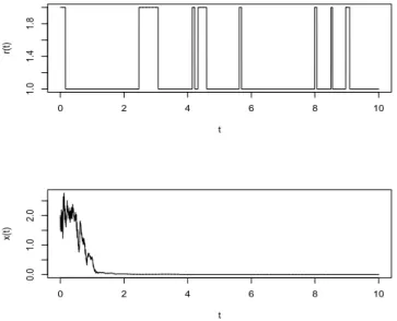
To perform computer simulations, we set σ1 = 0.8, σ2 = 1.2, τ = 0.1 and let the
initial data ξ(t) = 2 + sin(t) on t ∈ [−0.1,0] and r(0) = 2. The following computer simulations (Figure 6.1) support our theoretical results clearly.
0 2 4 6 8 10 1 .0 1. 4 1 .8 t r(t ) 0 2 4 6 8 10 0 .0 1 .0 2 .0 t x(t )
Figure 6.1: The computer simulations of the sample paths of the Markov chain and the solution of equation (3.9) with the parameters and initial data specified above using the
Euler–Maruyama method with step size 10−3.
6.3
Case 3
In this case we will discuss the robust boundedness. Assume that
xTF(x, t, i)≤ai1−ai2|x|2, i∈S1 (6.19)
and
where allai1andai2 are positive numbers. Suppose that the perturbed system is described
by
dx(t) =F(x(t), t, r(t))dt+G(x(t−τ), t, r(t))dB(t), (6.21) and the perturbation coefficients satisfy
|G(y, t, i)| ≤ai3|y|2, i∈S1 (6.22)
and
|G(y, t, i)| ≤ai3|y|2 +ai4|y|q−p+2, i∈S2, (6.23)
where ai3 and ai4 are all nonnegative numbers. We aim to obtain upper bounds on them
so that the perturbed system (6.21) remains asymptotically bounded. It follows from these conditions that for i∈S1
xTF(x, t, i) + 0.5(q−1)|G(y, t, i)|2 ≤ai1−ai2|x|2+ 0.5(q−1)a13|y|2; (6.24) while for i∈S2 xTF(x, t, i) + 0.5(p−1)|G(y, t, i)|2 ≤ai1−ai2|x|q−p+2+ 0.5(p−1)ai3|y|2 + 0.5(p−1)ai4|y|q−p+2. (6.25)
If we compare these with (4.2) and (4.3) in Assumption 4.2, we might attempt to have
αi2 =−ai2 for i∈S1 and 0 fori∈S2.
Consequently, the matrix A defined by (4.4) becomes
A= diag(pa12,· · · , paN12,0,· · · ,0)−Γ.
But A might not be a nonsingular M-matrix. To avoid this, we can simply choose a pair of constants δ1 >0 and δ2 ∈(0,1) and re-arrange (6.25) as
xTF(x, t, i) + 0.5(p−1)|G(y, t, i)|2 ≤αi1 −δ1|x|2+ 0.5(p−1)ai3|y|2 −(1−δ2)ai2|x|q−p+2+ 0.5(p−1)ai4|y|q−p+2, (6.26) where αi1 = sup u≥0 ai1+δ1u2−δ2ai2uq−p+2 .
As a result, Assumption 4.2 is satisfied with
αi1 =ai1, αi2 =−ai2, αi3 = 0.5(q−1)ai3
for i∈S1 while
αi2 =−δ1, αi3 = 0.5(p−1)ai3,
αi4 = (1−δ2)ai2, αi5 = 0.5(p−1)ai4
fori∈S2 (and αi1 has been defined above). Hence, the matricesAand Din Assumption
4.3 become
and
D= diag(qa12,· · ·, qaN12)−(γij)i,j∈S1.
By Lemma 2.1 and the note below it, bothAand Dare nonsingular M-matrices. In other words, Assumption 4.3 is satisfied too. To apply Theorem 4.5, we once again choose β by (4.8) so condition (4.9) is satisfied by Remark 4.4. Compute θi’s and byηi’s by (4.6) and
(4.7), respectively. Conditions (4.10)–(4.12) then become
ai3 ≤ 2 p(q−1)θi , ai3 < 2β (q−1)(2q−p)ηi for i∈S1 (6.27) and ai3 ≤ 2 p(p−1)θi , ai4 < 2qβ p(p−1)(2q−p)θi for i∈S2. (6.28)
By Theorems 4.5, we can therefore conclude that if the perturbed parameters αi3 satisfy
(6.15) and (6.16), then for any initial data ξ ∈ C([−τ,0];Rn), the solution x(t) of the
SDDE (6.21) has properties (4.13) and (4.14).
Example 6.2 Consider a scalar stochastically perturbed hybrid system
dx(t) =F(x(t), t, r(t))dt+G(x(t−τ), t, r(t))dB(t), (6.29) whereB(t) is a scalar Brownian,r(t) is a Markov chain with the state spaceS ={1,2,3,4} and the generator
Γ = −8 1 4 3 1 −6 2 3 1 1 −3 1 1 1 0 −2 ,
and the coefficients are defined by
F(x, t, i) = cost−2x, i= 1, sint−3x, i= 2, cost−2x3, i= 3, sint−3x3, i= 4 and G(y, t, i) = σ1y, i= 1, σ2y, i= 2, σ3y2, i= 3, σ4y2, i= 4.
Let S1 = {1,2}, S2 = {3,4} and p = 2, q = 4. It is straightforward to show that conditions (6.19), (6.20), (6.22) and (6.23) are satisfied with
a12= 1.9, a22 = 2.9, a32= 1.9, a42 = 2.9, a13=σ12, a23=σ22, a33 = 0, a43 = 0, a34=σ32, a44=σ24,
and ai1’s are all positive numbers but their values are of no further use so we do not
specify them. Choose two free parameters δ1 = 10 and δ2 = 0.1. Then
A= 11.8 −1 −4 −3 −1 11.8 −2 −3 −1 −1 13 −1 −1 −1 0 12 and D= 15.6 −1 −1 17.6 .
Noting that A−1 = 0.091 0.013 0.030 0.028 0.011 0.089 0.017 0.027 0.009 0.009 0.081 0.011 0.009 0.009 0.004 0.088 and D−1 = 0.064 0.004 0.004 0.057 ,
we see, by Lemma 2.1, that both A and D are nonsingular M-matrices. We can then compute
θ1 = 0.162, θ2 = 0.144, θ3 = 0.110, θ4 = 0.110,
˜
d= 0.068, γ˜ = 2, β = 0.331, η1 = 0.023, η2 = 0.020.
Conditions (6.27) and (6.28) then become
σ1 ≤1.264, σ2 ≤1.356, σ3 <1.416, σ4 <1.416. (6.30) We can therefore conclude that if the perturbed parameters σi satisfy (6.30), then for any
initial dataξ∈C([−τ,0];R), the solutionx(t) of the SDDE (6.29) has the properties that lim sup t→∞ 1 t Z t 0 E|x(s)|4ds≤K1, and lim sup t→∞ E|x(t)|2 ≤K2,
where K1 and K2 are positive constants independent of the initial dataξ.
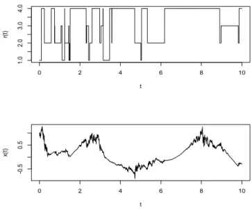
To perform a computer simulation for the second moment of the solution, we set
σ1 = 1,σ2 =σ3 =σ4 = 1.3,τ = 0.1 and let the initial dataξ(t) = 1+sin(t) ont ∈[−0.1,0] and r(0) = 1. The computer simulations in Figure 6.2 show a single sample path of the Markov chain and that of the solution, from which we can see how the Markov chain jumps from one mode to another and also the solution evolves in a bounded domain. To illustrate the boundedness of the second moment, we perform 200-sample-path simulations and then compute the average of their squares to form the approximation ofE|x(t)|2. This
is showed in Figure 6.3.
7
Conclusion
To distinguish the difference in structures of the underlying hybrid system, we have con-sidered the case where the space of modes, S, can be divided into two subspaces,S1 and
S2, such that the system is described by a same type of SDDEs for modes in S1 but by a different type of SDDEs for modes in S2. Taking these different structures into account we have successfully developed our new theory on the structured robust stability and boundedness for highly nonlinear hybrid SDDEs. A significant amount of new techniques has been developed to deal with the difficulties due to the structured difference and those without the linear growth condition. The proofs of Theorems 4.5 and 5.3 represent typ-ically our new techniques. We have also discussed three special cases and two examples plus some computer simulations to illustrate our theory.
0 2 4 6 8 10 1 .0 2 .0 3 .0 4 .0 t r(t ) 0 2 4 6 8 10 -0 .5 0 .5 t x(t )
Figure 6.2: The computer simulations of the sample paths of the Markov chain and the solution of equation (6.29) using the Euler–Maruyama method with step size 10−3.
0 2 4 6 8 10 0 .0 0 .2 0 .4 0 .6 0 .8 1 .0 t Ex^ 2 (t )
Figure 6.3: The computer simulation of the second moment of the solution of equation (6.29) using the Euler–Maruyama method with step size 10−3 and sample size 200.
Acknowledgements
The authors would like to thank the corresponding editor, associate editor and referees for their very helpful comments and suggestions. The authors would also like to thank the Royal Society (WM160014, Royal Society Wolfson Research Merit Award), the Royal So-ciety and the Newton Fund (NA160317, Royal SoSo-ciety-Newton Advanced Fellowship), the EPSRC (EP/K503174/1), the Natural Science Foundation of China (11471071, 71571001),
and the Ministry of Education (MOE) of China (MS2014DHDX020) for their financial support.
References
[1] Ackermann, J., Parameter space design of robust control systems, IEEE Trans. Au-tomat. Control 25 (1980), 1058–1080.
[2] Bahar, A. and Mao, X., Persistence of stochastic power law logistic model, Journal of Applied Probability and Statistics 3(1) (2008), 37–43.
[3] Basak, G.K., Bisi, A. and Ghosh, M.K., Stability of a random diffusion with linear drift,J. Math. Anal. Appl. 202 (1996), 604–622.
[4] Berman, A. and Plemmons, R.J.,Nonnegative Matrices in the Mathematical Sciences, SIAM, 1994.
[5] Costa, O.L.V., Assumpcao, E.O, Boukas, E.K, et al., Constrained quadratic state feedback control of discrete-time Markovian jump linear systems, Automatica 35(4)
(1999), 617–626.
[6] Haussmann, U.G., Asymptotic stability of the linear Itˆo equation in infinite dimen-sions, J. Math. Anal. Appl. 65 (1978), 219–235.
[7] Hinrichsen, D. and Pritchard, A.J., Stability radii of linear systems,Systems Control Lett. 7 (1986), 1–10.
[8] Hinrichsen, D. and Pritchard, A.J., A note on some differences between real and complex stability radii, Systems Control Lett. 14 (1990), 401–408.
[9] Hu, L., Mao, X. and Zhang, L., Robust stability and boundedness of nonlinear hy-brid stochastic differential delay equations,IEEE Transactions on Automatic Control
59(9) (2013), 2319–2332.
[10] Hu, L., Mao, X. and Shen, Y., Stability and boundedness of nonlinear hybrid stochas-tic differential delay equations, Systems and Control Letters 62 (2013), 178–187. [11] Ichikawa, A., Stability of semilinear stochastic evolution equations, J. Math. Anal.
Appl. 90 (1982), 12–44.
[12] Ji, Y. and Chizeck, H.J., Controllability, stabilizability and continuous-time Marko-vian jump linear quadratic control, IEEE Trans. Automat. Control 35 (1990), 777– 788.
[13] Ji, Y., Chizeck, H.J, Feng, X. et al., Stability and control of discrete-time jump linear systems, Contr. Theor. Adv. Tech. 7(2)(1991), 247–270.
[14] Khasminskii, R.Z.,Stochastic Stability of Differential Equations, Sijthoff and Noord-hoff, 1981.
[15] Lewis, A.L., Option Valuation under Stochastic Volatility: with Mathematica Code, Finance Press, 2000.
[16] Mao, X., Stability of Stochastic Differential Equations with Respect to Semimartin-gales, Longman Scientific and Technical, 1991.
[17] Mao, X., Exponential Stability of Stochastic Differential Equations, Marcel Dekker, 1994.
[18] Mao, X., Stochastic Differential Equations and Applications, 2nd Edition, Horwood Publishing, Chichester, 2007.
[19] Mao, X., Stability of stochastic differential equations with Markovian switching,Sto. Proc. Their Appl. 79 (1999), 45–67.
[20] Mao, X., Exponential stability of stochastic delay interval systems with Markovian switching, IEEE Trans. Auto. Control 47(10) (2002), 1604–1612.
[21] Mao, X., Koroleva, N. and Rodkina, A., Robust stability of uncertain stochastic differential delay equations, Systems Control Lett. 35(5)(1998), 325–336.
[22] Mao, X., Matasov, A. and Piunovskiy, A.B. , Stochastic differential delay equations with Markovian switching, Bernoulli 6(1) (2000), 73–90.
[23] Mao, X. and Yuan, C., Stochastic Differential Equations with Markovian Switching, Imperial College Press, 2006.
[24] Mariton, M.,Jump Linear Systems in Automatic Control, Marcel Dekker, 1990. [25] Shaikhet, L., Stability of stochastic hereditary systems with Markov switching,
The-ory of Stochastic Processes 2(18)(1996), 180–184.
[26] Su, J.-H., Further results on the robust stability of linear systems with a single time delay, Systems and Control Letters 23(1994), 375–379.
[27] Tseng, C.-L., Fong, I.-K. and Su, J.-H., Robust stability analysis for uncertain delay systems with output feedback controller, Systems Control Lett. 23 (1994), 271–278. [28] You, S., Liu, W., Lu, J., Mao, X. and Qiu, Q., Stabilization of hybrid systems by feedback control based on discrete-time state observations, SIAM J. Control and Optimization 53(2) (2015), 905–925.