The kernel Kalman rule: efficient nonparametric inference with recursive least squares

The Kernel Kalman Rule

– Efficient Nonparametric Inference with Recursive Least Squares

Gregor H.W. Gebhardt

CLAS, TU Darmstadt Hochschulstr. 10 64285 Darmstadt, Germany [email protected]

Andras Kupcsik

National University of Singapore

School of Computing

13 Computing Drive, Singapore 117417 [email protected]

Gerhard Neumann

School of Computer Science

University of Lincoln Lincoln, LN6 7TS, UK [email protected]

Abstract

Nonparametric inference techniques provide promising tools for probabilistic reasoning in high-dimensional nonlinear sys-tems. Most of these techniques embed distributions into re-producing kernel Hilbert spaces (RKHS) and rely on the ker-nel Bayes’ rule (KBR) to manipulate the embeddings. How-ever, the computational demands of the KBR scale poorly with the number of samples and the KBR often suffers from numerical instabilities. In this paper, we present thekernel Kalman rule(KKR) as an alternative to the KBR. The deriva-tion of the KKR is based on recursive least squares, inspired by the derivation of the Kalman innovation update. We apply the KKR to filtering tasks where we use RKHS embeddings to represent the belief state, resulting in thekernel Kalman fil-ter(KKF). We show on a nonlinear state estimation task with high dimensional observations that our approach provides a significantly improved estimation accuracy while the compu-tational demands are significantly decreased.

1

Introduction

State estimation and prediction for continuous partially ob-servable stochastic processes is a significant challenge in many high-dimensional applications, such as robotics. How-ever, analytical solutions are only applicable for a limited set of models with special structure. When assuming linear models with Gaussian noise, for instance, the Kalman fil-ter (Kalman 1960) is known to provide an optimal solution. For more complex models, approximate solutions have to be used instead (McElhoe 1966; Smith, Schmidt, and McGee 1962; Julier and Uhlmann 1997; Wan and Van Der Merwe 2000). These approximations are again difficult to scale to high-dimensional problems, they often assume a unimodal Gaussian observation prior and also require that the model of the system is known.

The recently introduced methods for nonparametric infer-ence (Song, Fukumizu, and Gretton 2013; Fukumizu, Song, and Gretton 2013) alleviate the problems of traditional state estimation methods for nonlinear systems. The idea of these methods is to represent probability distributions as points in reproducing kernel Hilbert spaces. Based on the kernel-ized versions of the sum rule, the chain rule, and the Bayes’ Copyright c2017, Association for the Advancement of Artificial Intelligence (www.aaai.org). All rights reserved.

rule, inference can be performed entirely in the RKHS. Ad-ditionally, Song, Fukumizu, and Gretton (2013) use the nel sum rule and the kernel Bayes’ rule to construct the ker-nel Bayes’ filter (KBF). The KBF learns the transition and observation models from observed samples and can be ap-plied to nonlinear systems with high-dimensional observa-tions. However, the computational complexity of the KBR update scales poorly with the number of samples such that hyper-parameter optimization becomes prohibitively expen-sive. Moreover, the KBR requires mathematical tricks that may cause numerical instabilities and also render the objec-tive which is optimized by the KBR unclear.

In this paper, we present thekernel Kalman rule(KKR) as alternative to the kernel Bayes’ rule. Our derivations closely follow the derivations of the innovation update used in the Kalman filter and are based on a recursive least squares min-imization objective in a reproducing kernel Hilbert space. We show that our update of the mean embedding is unbi-ased and has minimum variance. While the update equations are formulated in a potentially infinite dimensional RKHS, we derive, through the application of the kernel trick and by virtue of the representer theorem (Sch¨olkopf, Herbrich, and Smola 2001), an algorithm using only products and in-versions of finite kernel matrices. We employ the kernel Kalman rule together with the kernel sum rule for filtering, which results in the kernel Kalman filter (KKF). In contrast to filtering techniques that rely on the KBR, the KKF allows to precompute expensive matrix inversions which signifi-cantly reduces the computational complexity. This allows us also to apply hyper-parameter optimization for the KKF.

To scale gracefully with larger data sets, we rederive the KKR and the KKF with the subspace conditional operator (Gebhardt, Kupcsik, and Neumann 2015). Here, only a sub-set of the samples is used to span a feature space, while all training samples are used to estimate the models.

We compare our approach to different versions of the KBR and demonstrate its improved estimation accuracy and computational efficiency. Furthermore, we evaluate the KKR on a simulated 4-link pendulum task and a human mo-tion capture data set (Wojtusch and von Stryk 2015).

1.1

Related Work

To the best of our knowledge, the kernel Bayes’ rule ex-ists in three different versions. It was first introduced in its

original version by Fukumizu, Song, and Gretton (2013). Here, the KBR is derived, similar to the conditional oper-ator, using prior modified covariance operators. These prior-modified covariance operators are approximated by weight-ing the feature mappweight-ings with the weights of the embed-ding of the prior distribution. Since these weights are po-tentially negative, the covariance operator might become indefinite which renders its inversion impossible. To over-come this drawback, the authors have to apply a form of the Tikhonov regularization that significantly decreases ac-curacy and increases the computational costs. A second ver-sion of the KBR was introduced by Song, Fukumizu, and Gretton (2013) in which they use a different approach to ap-proximate the prior-modified covariance operator. In the ex-periments conducted for this paper, this second version often leads to more stable algorithms than the first version. Boots, Gretton, and Gordon (2013) introduced a third version of the KBR where they apply only the simple form of the Tikhonov regularization. However, this rule requires the inversion of a matrix that is often indefinite, and therefore, high regu-larization constants are required, which again degrades the performance. In our experiments, we refer to these different versions with KBR(b) for the first, KBR(a) for the second (both adapted from the literature), and KBR(c) for the third version.

For filtering tasks with known linear system equations and Gaussian noise, the Kalman filter (KF) yields the so-lution that minimizes the squared error of the estimate to the true state. Two widely known and applied approaches to ex-tend the Kalman filter to non-linear systems are theextended Kalman filter(EKF) (McElhoe 1966; Smith, Schmidt, and McGee 1962) and theunscented Kalman filter(UKF) (Wan and Van Der Merwe 2000; Julier and Uhlmann 1997). Both, the EKF and the UKF, assume that the non-linear system dynamics are known and use them to update the prediction mean. Yet, updating the prediction covariance is not straight-forward. In the EKF the system dynamics are linearized at the current estimate of the state, and in the UKF the co-variance is updated by applying the system dynamics to a set of sample-points (sigma points). While these approxima-tions make the computaapproxima-tions tractable, they can significantly reduce the quality of the state estimation, in particular for high-dimensional systems.

Hsu, Kakade, and Zhang (2012) recently proposed an al-gorithm for learning Hidden Markov Models (HMMs) by exploiting the spectral properties of observable measures to derive an observable representation of the HMM (Jaeger 2000). An RKHS embedded version thereof was presented in (Song et al. 2010). While this method is applicable for continuous state spaces, it still assumes a finite number of discrete hidden states.

Other closely related algorithms to our approach are the kernelized version of the Kalman filter by Ralaivola and d’Alche Buc (2005) and the kernel Kalman filter based on the conditional embedding operator (KKF-CEO) by Zhu, Chen, and Principe (2014). The former approach formulates the Kalman filter in a sub-space of the infinite feature space that is defined by the kernels. Hence, this approach does not fully leverage the kernel idea of using an infinite

fea-ture space. In contrast, the KKF-CEO approach embeds the belief state also in an RKHS. However, they require that the observation is a noisy version of the full state of the system, and thus, they cannot handle partial observations. Moreover, they also deviate from the standard derivation of the Kalman filter, which, as our experiments show, decreases the estima-tion accuracy. The full observability assumpestima-tion is needed in order to implement a simplified version of the innovation update of the Kalman filter in the RKHS. The KKF does not suffer from this restriction. It also provides update equa-tions that are much closer to the original Kalman filter and outperforms the KKF-CEO algorithm as shown in our ex-periments.

2

Preliminaries

Our work is based on embeddings of probability densities into reproducing kernel Hilbert spaces (RKHS). For a de-tailed survey see the work of Song, Fukumizu, and Gret-ton (2013). An RKHSHkis a Hilbert space associated with

an inner producth·,·ithat is implicitly defined by a kernel functionk : Ω×Ω → Rashϕ(x),ϕ(x0)i := k(x,x0).

Here,ϕ(x)is a feature mapping into a possibly infinite di-mensional space, intrinsic to the kernel function. The ker-nel functionksatisfies the reproducing property (Aronszajn 1950), i.e.,f(x) =hf,ϕ(x)ifor anyf ∈ Hk.

A marginal density P(X) over the random variableX can be embedded as the expected feature mapping (or mean map)µ_X :=EX[ϕ(X)](Smola et al. 2007). Using a finite

set of samples fromP(X), the mean map can be estimated as

ˆ

µ_X= _m1 Pm

i=1ϕ(xi) = _m1Υ|x1m, (1)

whereΥx = [ϕ(x1), . . . ,ϕ(xm)]is a matrix consisting of

the feature mappings of the samples and1m ∈ Rm is an

mdimensional all-ones vector. Alternatively, a distribution can be embedded in a tensor product RKHS Hk × Hk as

the expected tensor product of the feature mappings, i.e.,

CXX := EXX[ϕ(X)⊗ϕ(X)]−µX ⊗µX (Smola et al.

2007). This embedding is also called the centered covariance operator. The finite sample estimator is given by

ˆ

CXX =_m1 Pmi=1ϕ(xi)⊗ϕ(xi)−µˆX⊗µˆX. (2)

Similarly, we can define the (uncentered) cross-covariance operator for a joint distributionp(X, Y)of two variablesX andY asCˆXY = _m1 Pm_i=1ϕ(xi)⊗φ(yi). Here,φ(·)is the

intrinsic feature mapping of another kernel function defined on the Cartesian product of the domain ofy.

The embedding of a conditional distributionP(Y|X)is defined as a conditional embedding operatorCY|Xthat

satis-fiesµ_Y|x:=EY|x[φ(Y)] =CY|Xϕ(x)(Song, Fukumizu,

and Gretton 2013). Given a finite set of samples, the condi-tional embedding operator can be estimated as

ˆ

CY|X =Φy(Kxx+λIm)−1Υ|x, (3)

with the feature mappingsΦy := [φ(y1), . . . ,φ(ym)], the

Gram matrixKxx = Υ|xΥx ∈ Rm×m, the regularization

The kernel Bayes’ rule (KBR) infers the mean em-bedding µπ_X|y of the posterior distribution Q(X|Y) = P(Y|X)π(X)/P

XP(Y|X)π(X). It uses the kernel sum

and the kernel chain rule to obtain the prior-modified co-variance operatorsCπ

Y Y andCY Xπ . For a more detailed

dis-cussion of these operators, we refer to Song, Fukumizu, and Gretton (2013). There exist, to the authors’ knowl-edge, three different versions of the KBR. In the first ver-sion of the KBR, Fukumizu, Song, and Gretton (2013) used the tensor product conditional operator in the kernel chain rule, i.e., µˆπ_X|y = ΥxDGyy (DGyy)2+κIm−

1

Dg_y,

with the diagonal D := diag((Kxx +λIm)−1Kxxα),

the Gram matrix Gyy = Φ|yΦy, the kernel vector

g_y and κ as regularization parameter. Song, Fukumizu, and Gretton (2013) additionally derived the KBR, us-ing an alternative formulation of the kernel chain rule, as µˆπ_X|y = ΥxΛ| (DGyy)2+κIm−

1

GyyDgy, with

Λ:= (Kxx+λIm)−1Kxxdiag(α). As the matrixDGyy

is typically not invertible, both of these versions of the KBR use a form of the Tikhonov regularization in which the matrix in the inverse is squared. Boots, Gretton, and Gordon (2013) use a third form of the KBR which is de-rived analogously to the first version but does not use the squared form of the Tikhonov regularization, i.e.,µˆπ_X|y = Υx(DGyy+κIm)−1Dgy. Since the product DGyy is

often not positive definite, a strong regularization parame-ter is needed to make the matrix invertible.

All three versions of the kernel Bayes’ rule presented above have drawbacks. First, due to the approximation of the prior modified covariance operators, these operators are not guaranteed to be positive definite and, thus, their inver-sion requires either a harsh form of the Tikhonov regular-ization or a strong regularregular-ization factor and are often still numerically instable. Furthermore, the inverse is dependent on the embedding of the prior distribution and, hence, needs to be recomputed for every Bayesian update of the mean map. This recomputation significantly increases the com-putational costs, for example, if we want to apply hyper-parameter optimization techniques.

3

The Kernel Kalman Rule

In this section, we will present a new approach to Bayesian reasoning in Hilbert spaces inspired by recursive least squares estimation (Gauss 1823; Sorenson 1970; Simon 2006). That is, we want to infer the embedding of a dis-tribution µ+_X,t = EXt|y1:t[ϕ(X)] a-posteriori to a new measurement yt, given the embedding of the distribution

µ−_X,t =_EXt|y_1:t−1[ϕ(X)]a-priori to the measurement. We

assume a conditional embedding operatorCY|Xof the

distri-butionP(Y|X)as given. Usually, this conditional operator can be estimated from a training set of state-measurement-pairs{(xi,yi)}mi=1.

3.1

Recursive Least Squares for Estimating the

Posterior Embedding

The derivations for thekernel Kalman rule (KKR) are in-spired by the ansatz from recursive least squares. Hence, the

objective of the KKR is to find the mean embeddingµ_Xthat

minimizes the squared error

P t φ(yt)− CY|XµX | R−1 _φ(y t)− CY|XµX , (4) with the metricR, in an iterative fashion. In each iteration,

we want to update the prior mean map µ−_X,t based on the

measurementy_tto obtain the posterior mean mapµ+_X,t.

From the recursive least squares solution, we know that the update rule for obtaining the posterior mean mapµ+_X,tis µ+_X,t=µ−_X,t+Qt(φ(yt)− CY|Xµ−X,t), (5)

whereQtis the Hilbert space Kalman gain operator that is

applied to the correction termδt=φ(yt)− CY|Xµ−X,t.

We denote the error of the a-posteriori estimator to the embedding of the true state asε+_t =ϕ(xt)−µ+X,t, and

anal-ogously, the error of the a-priori estimator asε−_t. It is easy

to show that the kernel Kalman update, given an unbiased a-priori estimator (E[ε−t] = 0), yields an unbiased a-posteriori

estimator (E[ε+t] = 0), independent of the choice ofQt. For

an elaborate discussion of the unbiasedness, we refer to the supplement. Yet, we want to obtain the kernel Kalman gain operatorQtthat minimizes the squared loss which is

equiv-alent to minimizing the variance of the estimator. The objec-tive of minimizing the variance can be written as minimizing the trace of the a-posteriori covariance operatorC_XX,t+ of the statextat timet, i.e.,

min_QtE ε+_t| ε+_t = min_QtTr_E ε+_t ε+_t| (6) = min_QtTrC_XX,t+ .

Since the measurement residualtis assumed to be

inde-pendent from the estimation error, and by substituting the posterior error with ε+_t = (I − QtCY|X)ε−t − Qtt, the

posterior covariance operator can be reformulated as

C_XX,t+ = I − QtCY|X

C_XX,t− I − QtCY|X

|

+QtRQ|t, (7)

whereRis the covariance of the measurement residual.

Tak-ing the derivative of the trace of the covariance operator and setting it to zero leads to the following solution for the kernel Kalman gain operator

Qt=C_XX,t− C_Y|_|X(CY|XCXX,t− C|Y|X+R)−

1_{. (8)}

From Eqs. 7 and 8, we can also see that it is possible to recursively estimate the covariance embedding operator in-dependently of the mean map or of the observations. This property will allow us later to precompute the covariance embedding operator as well as the kernel Kalman gain oper-ator to further improve the computational complexity of our algorithm.

3.2

Empirical Kernel Kalman Rule

In practice, the conditional observation operator and the ker-nel Kalman gain operator are estimated from a finite set of samples. Applying the kernel trick (i.e., matrix identities) renders the kernel Kalman rule computationally tractable.

In general, an estimator of the prior mean embedding is given asµˆ−_X,t = Υxm−t, with weight vectorm−t, and an

estimator of the covariance operator is given as _Cˆ−

XX,t =

ΥxS−tΥ|x, with positive definite weight matrixS−t.

We can rewrite the kernel Kalman gain operator by sub-stituting with the estimators of the covariance operator and of the conditional operator (c.f. Eq. 3) and obtain

Qt=ΥxS−tO|Φy|(ΦyOS−tO|Φy|+κI)−1, (9)

with O = (Kxx +λOIm)−1Kxx and with the

simpli-fication R = κI. However, Qt still contains the

inver-sion of an infinite dimeninver-sional matrix. We can solve this problem by applying the matrix identityA(BA+I)−1 = (AB+I)−1Aand arrive at

Qt=ΥxS−tO|(GyyOS−tO|+κIm)−1Φy|

=ΥxQtΦy|, (10)

withQ_t = S−_tO|(GyyOSt−O| +κIm)−1 andGyy =

Φ|_yΦy. We can now use this reformulation of the kernel

Kalman gain operator and apply it to the update equations for the estimator of the mean embedding (Eq. 5) and the es-timator of the covariance operator (Eq. 7). It is now straight forward to obtain the update equations for the weight vector

mtand the weight matrixStas

m+_t =m−_t +Q_t(g_:y t−GyyOm − t), (11) S+_t =S−_t −Q_tGyyOS−t, (12) whereg_:y t = Φ |

yφ(yt)is the embedding of the

measure-ment at time t. The algorithm requires the inversion of a m×m matrix in every iteration for computing the kernel Kalman gain matrixQ_t. Hence, similar to the kernel Bayes’

rule, the computational complexity of a straightforward im-plementation would scale cubically with the number of data pointsm. However, in contrast to the KBR, the inverse in

Q_tis only dependent on time and not on the estimate of the

mean map. The kernel Kalman gain matrix can, thus, be pre-computed as it is identical for multiple parallel runs of the algorithm. While many applications do not require parallel state estimations, it is a huge advantage for hyper-parameter optimization as we can evaluate multiple trajectories from a validation set simultaneously. As for most kernel-based methods, hyper-parameter optimization is crucial for scaling the approach to complex tasks. So far, the hyper-parameters of the kernels for the KBF have typically been set by heuris-tics as optimization would be too expensive.

3.3

The Subspace Kernel Kalman Rule

The computational complexity of non-parametric inference suffers from a polynomial growth with the number of sam-ples used for estimating the embeddings. To overcome this drawback, several approaches exist that aim to find a good trade-off between a compact representation and leverag-ing from a large data set (Snelson and Ghahramani 2006; Csat and Opper 2002; Smola and Bartlett 2001; Gebhardt, Kupcsik, and Neumann 2015). In the following paragraphs, we will explain how the concept of subspace conditional operators (Gebhardt, Kupcsik, and Neumann 2015) can be

applied to the kernel Kalman rule in order to maintain the update rules also for large training sets computationally tractable without ignoring valuable information from the provided training samples.

The subspace conditional operator uses subspace pro-jections as representations of the mean map nt =

Υ_ˆx|µt = Υx|ˆΥxmt and the covariance operator Pt =

Υ|_ˆxCXX,tΥxˆ = Υ|_ˆxΥxStΥ|xΥˆx, whereΥxˆ is the feature

matrix of a sparse reference set. The subspace conditional operator of the distributionP(Y|X)is then given as

C_Ys_|X =ΦyKxxˆ(Kxxˆ Kxxˆ+λxˆIn)−1Υxˆ|, (13) whereKxxˆ = Υx|ˆΥx ∈ Rn×m is the kernel matrix

be-tween the sparse subset and the full training data. Using the subspace conditional operator and the subspace representa-tion of the covariance embedding in the kernel Kalman gain operator, we arrive at the following finite representation of the subspace kernel Kalman gain operator

Qs_t=P−_tLs Kxxˆ GyyKxˆxLsP−tLs+κIn

−1

Kˆxx,

withLs = (Kxxˆ Kxˆx+λIn)−1. For a detailed derivation

ofQs_t, we refer to the supplement. By analogously applying

the subspace representations to the update equations for the mean map and the covariance operator, we obtain

n+_t =n−_t +Qs_t g(yt)−GyyKxxˆLsn−t

, (14)

P+_t =P−_t −Qs_tGyyKxxˆLsP−t. (15)

3.4

Recovering the State-Space Distribution

Recovering a distribution in the state space that is a valid preimage of a given mean map is still a topic of ongoing re-search. There are several approaches to this problem, such as fitting a Gaussian mixture model (McCalman, O ’Callaghan, and Ramos 2013), or sampling from the embedded distri-bution by optimization (Chen, Welling, and Smola 2010). In the experiments conducted for this paper, we approached the preimage problem by matching a Gaussian distribution, which is a reasonable choice if the recovered distribution is unimodal. Since the belief state of the kernel Kalman rule is a mean map as well as a covariance operator, obtaining the mean and covariance of a Gaussian approximation is done by simple matrix manipulations. For more details we refer to the supplement. However, also any other approach from the literature can be used with the KKR.

3.5

The Kernel Kalman Filter

Similar to the kernel Bayes’ filter (Fukumizu, Song, and Gretton 2013; Song, Fukumizu, and Gretton 2013), we can combine the kernel Kalman rule with the kernel sum rule to formulate thekernel Kalman filter. We assume a data set

{(¯x1, x1, y1), . . . ,(¯xm, xm, ym)}consisting of triples with

preceding statex¯i, statexi, and measurementyi as given.

Based on this data set we can define the feature matrices Υx = [ϕ(x1), . . . ,ϕ(xm)], Υ¯x = [ϕ(¯x1), . . . ,ϕ(¯xm)],

andΦy= [φ(y1), . . . ,φ(ym)]. We represent the belief state

as a mean map µˆX,t = Υxmt and a covariance

opera-tor_Cˆ_{XX,t =ΥxStΥ}|

conditional embeddings for the distributionsP(X|X¯)and P(Y|X)as

C_X|X¯ =Υx(Kx¯x¯+λTI)−1Υ|x¯ and (16) CY|X =Φy(Kxx+λOI)−1Υ|x, (17)

respectively. We can propagate the posterior belief state at timetto the prior belief state at timet+ 1time by applying the kernel sum rule to the mean embedding and the covari-ance embedding and obtain the following update rules

m−_t+1=T m+_t, S_t−₊₁=T S+_tT|+V, (18) withT = (K¯xx¯+λTI)−1Kxx¯ . Subsequently, we can use

the kernel Kalman rule to obtain a posterior belief from the prior embedding conditioned on a new measurement follow-ing the steps described in Section 3.2.

4

Experimental Results

In this section, we give a concise description of the experi-ments we conducted to evaluate the performance of the ker-nel Kalman rule. In a first experiment, we compare only the kernel Kalman rule to the kernel Bayes’ rule by applying them to a simple estimation task. In the further experiments, we compare the kernel Kalman filter to other filtering meth-ods. For these evaluations we use time series from two simu-lated environments, a simple pendulum and a quad-link, and time series from a human motion tracking data set (Wojtusch and von Stryk 2015). For all kernel based methods, we use the squared exponential kernel. We choose the kernel band-widths according to the median trick(Jaakkola, Diekhans, and Haussler 1999) and scale the found median distances with a single parameter that is optimized.

4.1

Estimation of an Expectation of a Gaussian

Distribution

In a first simple experiment, we compare the kernel Kalman rule to the kernel Bayes’ rule. We train the models with data sets consisting of hidden states, sampled uniformly from the interval [−2.5,2.5], and the corresponding mea-surements, where we add Gaussian noise with standard de-viationσ= 0.3. The training set consists of 100 samples for the KKR and KBR and 500 samples for the subspace KKR, where we still use100samples as reference set. We estimate the hidden state by a conditional operator that maps from the kernel space back to the original state. Figure 1 shows the mean squared error (MSE) of the estimated hidden state to

2 4 6 8 10 0.00 0.05 0.10 # of updates MSE KKR subKKR KBR(a) KBR(c) ML

Figure 1: Estimating the expectation of a Gaussian distribu-tion with KKR and KBR. The reference is the expected error of a maximum likelihood estimator.

KKR subKKR KBR(a) KBR(b) KBR(c) 0.0813 s 0.1074 s 1.2149 s 0.8643 s 0.5655 s Table 1: Mean time consumed for performing 10 updates on 100 estimates (in parallel) over 20 runs.

the true hidden state for 10 iterative updates with new mea-surements. The graphs depict mean and 2σ intervals over 20 evaluations. We conducted this experiment with all three versions of the KBR, however, version (b) was numerically instable which led to MSEs that did not fit into the plot any-more. We can see that the estimates from the KKR and the subKKR are at the level of the ML estimator, while the KBR has a worse performance which is not improving with the number of updates. In addition, we limit the values in theD

matrix for the KBRs to only positive values in order to get reasonable results.

In Table 1, we compare the computational efficiency of the KKR to the KBR. The times shown are the mean times for 10 updates of 100 estimates. While the single updates could be performed in parallel with the KKR and the sub-KKR, they have to be performed for each estimate indepen-dently for the KBR. It can be clearly seen that the KKR out-performs the KBR in the order of a magnitude. Furthermore, the subKKR maintains computational efficiency, while us-ing 5 times more data points for learnus-ing the models.

4.2

Pendulum

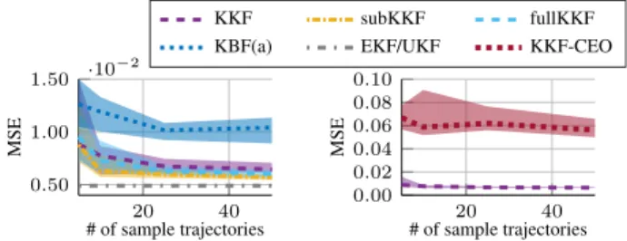
In this experiment, we use a simulated pendulum as system dynamics. It is uniformly initialized in the range[0.1π,0.4π] with a velocity sampled from the range[−0.5π,0.5π]. The observations of the filters were the joint positions with addi-tive Gaussian noise sampled fromN(0,0.01). We compare the KKF, the subspace KKF (subKKF) and the KKF learned with the full dataset (fullKKF) to version (a) of the kernel Bayes filter (Song, Fukumizu, and Gretton 2013), the kernel Kalman filter with covariance embedding operator (KKF-CEO) (Zhu, Chen, and Principe 2014), as well as to standard filtering approaches such as the EKF (Julier and Uhlmann 1997) and the UKF (Wan and Van Der Merwe 2000). Both, the EKF and the UKF require a model of the system dy-namics. KBF(b) was numerically too instable and KBF(c) already yielded worse results in the previous experiment. To learn the models, we simulated episodes with a length of 30 steps (3s). The results are shown in Figure 2. The KKF and subKKF show clearly better results than all other non-parametric filtering methods and reach a performance level close to the EKF and UKF.

4.3

Quad-Link

In this experiment, we used a simulated 4-link pendulum where we observe the 2-D end-effector positions. The state of the pendulum consists of the four joint angles and joint velocities. We evaluate the prediction performance of the subKKF in comparison to the KKF-CEO, the EKF and the UKF. All other non-parametric filtering methods could not achieve a good performance or broke down due to the high computation times. As the subKKF outperformed the KKF

20 40 0.50 1.00 1.50 ·10− 2 # of sample trajectories MSE KKF subKKF fullKKF

KBF(a) EKF/UKF KKF-CEO

20 40 0.00 0.02 0.04 0.06 0.08 0.10 # of sample trajectories MSE

Figure 2: Comparison of KKF to KBF(a), KKF-CEO, EKF and UKF. All kernel methods (except fullKKF) use kernel matrices of 100 samples. The subKKF method uses a subset of 100 samples and the whole dataset to learn the conditional operators. Depicted is the median MSE to the ground-truth of 20 trials with the [0.25 0.75] quantiles.

(a) anim. QL (b) MCF (c) UKF (d) subKKF Figure 3: Example trajectory of the quad-link end-effector. The filter outputs in black, where the ellipses enclose 90% of the probability mass. All filters were updated with the first five measurements (yellow marks) and predicted the follow-ing 30 steps. Figure (a) is an animation of the trajectory. in the previous experiments and is also computationally much cheaper, we skip the comparison to the standard KKF in this and the subsequent experiments.

In a first qualitative evaluation, we compare the long-term prediction performance of the subKKF in comparison to the UKF, the EKF and the Monte-Carlo filter (MCF) as a base-line (see Appendix). This evaluation can be seen in Figure 3. The UKF is not able to predict the movements of the quad-link end-effector due to the high non-linearity, while the sub-KKF is able to predict the whole trajectory.

We also compared the 1, 2 and 3-step prediction perfor-mance of the subKKF to the KKF-CEO, EKF and UKF (Fig. 4). The KKF-CEO provides poor results already for the filtering task. The EKF performs equally bad, since the observation model is highly non-linear. The UKF already yields a much better performance as it does not suffer from the linearization of the system dynamics. The subKKF out-performed the UKF.

t t+ 1 t+ 2 t+ 3 0 0.2 0.4 0.6 prediction steps MED subKKF KKF-CEO EKF UKF

Figure 4: 1, 2 and 3 step prediction performances in mean euclidean distances (MED) to the true end-effector positions of the quad-link.

Figure 5: Example sequence of 4 postures. The markers of the upper body (violet circles) were observed and the posi-tions of all markers (yellow crosses) and of all joints (yellow skeleton) were estimated. The black skeleton is the ground-truth from the dataset.

0 200 400 600 0 1 2 3 4 timestep velocity [ m]s Figure 6: Estimated subject velocity of the human motion dataset by the subKKF (or-ange) and ground-truth (blue).

4.4

Human Motion Dataset

We used walking and running motions captured from one subject from the HuMoD dataset (Wojtusch and von Stryk 2015). The dataset comprised the x, y and z locations of the 36 markers attached to the subject’s body as well as the ve-locity of the subject in x-direction, computed from the mark-ers at the left and right anterior-superior iliac spine. We used walking and running motions at different constant speeds for training one model. For the evaluation of this model, we used a test data-set in which the subject accelerates from 0m/s to 4m/s.

In a first experiment, we learned the subKKF with a ker-nel size of 800 samples, where we used data windows of size 3 with the 3D positions of all 36 markers as state representa-tion and the current 3D posirepresenta-tions of all markers as observa-tions. In this task, we want to predict the subject’s velocity. To do so, we learned a conditional operator from the state representation to the observed velocities in the training set. Subsequently, we applied our model to the transition motion dataset to reconstruct the subject’s velocity. The results of this experiment are depicted in Figure 6.

In a second experiment, we learned the subKKF with a kernel size of 2000 samples and used data windows of size 4 with all 36 marker positions as state representations. How-ever, this time we observed only the markers on the upper body and used all marker positions as well as the joint po-sitions as prediction targets. Figure 5 shows a sequence of 4 postures, where the blue circles denote the observation, the red crosses the reconstructed positions of the markers, the red skeleton is drawn with the reconstructed positions of the joints and the black skeleton is drawn with the joint positions in the dataset.

5

Conclusions

In this paper, we proposed the kernel Kalman rule (KKR) for Bayesian inference with nonparametric representations of probability distributions. We showed that the KKR, as an alternative to the kernel Bayes’ rule (KBR), is compu-tationally more efficient, numerically more stable and fol-lows from a clear optimization objective. We combined the

KKR as Bayesian update with the kernel sum rule to for-mulate the kernel Kalman filter (KKF) that can be applied to nonlinear filtering tasks. In difference to existing kernel Kalman filter formulations, the KKF provides a more gen-eral formulation that is much closer to the original Kalman filter equations and can also be applied to partially observ-able systems. Future work will concentrate on the use of hyper-parameter optimization with more complex kernels and learning the transition dynamics in the RKHS with an expectation-maximization algorithm in case of missing in-formation about the latent state.

Acknowledgments

This project has received funding from the European Unions Horizon 2020 research and innovation program under grant agreement No #645582 (RoMaNS).

Appendix

We use a Monte Carlo approach to compare the KKF to a baseline in the quadlink prediction task (c.f. Sec. 4.3). We sample105episodes from the known system equations and use the knowledge about the observation noise to compute the likelihood of the observations w.r.t. each of the sampled episodes. We can then obtain a posterior of each sampled episode given the observations by normalizing the likeli-hood. We weigh each of the sampled episodes with its pos-terior probability and obtain finally the Monte Carlo filter output as the sum of these weighted episodes.

References

Aronszajn, N. 1950. Theory of reproducing kernels.Transactions of the American Mathematical Society68(3):337–404.

Boots, B.; Gretton, A.; and Gordon, G. J. 2013. Hilbert space em-beddings of predictive state representations. InProceedings of the 29th International Conference on Uncertainty in Artificial Intelli-gence (UAI).

Chen, Y.; Welling, M.; and Smola, A. J. 2010. Supersamples from kernel-herding. InProceedings of the 26th International Confer-ence on Uncertainty in Artificial IntelligConfer-ence (UAI).

Csat, L., and Opper, M. 2002. Sparse on-line gaussian processes. Neural computation14(3):641–668.

Fukumizu, K.; Song, L.; and Gretton, A. 2013. Kernel bayes’ rule: Bayesian inference with positive definite kernels. Journal of Machine Learning Research14(1):3683–3719.

Gauss, C. F. 1823.Theoria combinationis observationum erroribus minimis obnoxiae. H. Dieterich.

Gebhardt, G. H. W.; Kupcsik, A.; and Neumann, G. 2015. Learning subspace conditional embedding operators. Workshop on Large-Scale Kernel Learning at ICML 2015.

Hsu, D.; Kakade, S. M.; and Zhang, T. 2012. A spectral algorithm for learning hidden markov models.Journal of Computer and Sys-tem Sciences78(5):1460–1480.

Jaakkola, T.; Diekhans, M.; and Haussler, D. 1999. Using the fisher kernel method to detect remote protein homologies. InProceedings of the Seventh International Conference on Intelligent Systems for Molecular Biology, 149–158.

Jaeger, H. 2000. Observable operator models for discrete stochastic time series.Neural Computation12(6):1371–1398.

Julier, S. J., and Uhlmann, J. K. 1997. A new extension of the kalman filter to nonlinear systems. InInt. symp. aerospace/defense sensing, simul. and controls, volume 3, 3–2.

Kalman, R. E. 1960. A new approach to linear filtering and pre-diction problems.Journal of Fluids Engineering82(1):35–45. McCalman, L.; O ’Callaghan, S.; and Ramos, F. 2013. Multi-modal estimation with kernel embeddings for learning motion models. In Robotics and Automation (ICRA), 2013 IEEE International Con-ference on, 2845–2852. Karlsruhe: IEEE.

McElhoe, B. A. 1966. An assessment of the navigation and course corrections for a manned flyby of mars or venus. IEEE Transac-tions on Aerospace and Electronic SystemsAES-2.

Ralaivola, L., and d’Alche Buc, F. 2005. Time series filtering, smoothing and learning using the kernel kalman filter. Proceed-ings. 2005 IEEE International Joint Conference on Neural Net-works, 2005.3:1449–1454.

Sch¨olkopf, B.; Herbrich, R.; and Smola, A. 2001. A generalized representer theorem.Computational Learning Theory(2111):416– 426.

Simon, D. 2006. Optimal State Estimation. Hoboken, NJ, USA: John Wiley & Sons, Inc.

Smith, G. L.; Schmidt, S. F.; and McGee, L. A. 1962.Application of statistical filter theory to the optimal estimation of position and velocity on board a circumlunar vehicle. National Aeronautics and Space Administration.

Smola, A. J., and Bartlett, P. 2001. Sparse greedy gaussian process regression. Advances in Neural Information Processing Systems 13:619–625.

Smola, A. J.; Gretton, A.; Song, L.; and Sch¨olkopf, B. 2007. A hilbert space embedding for distributions. InProceedings of the 18th international conference on Algorithmic Learning Theory, volume 4754, 13–31.

Snelson, E., and Ghahramani, Z. 2006. Sparse gaussian processes using pseudo-inputs. InAdvances in Neural Information Process-ing Systems 18, 1257–1264.

Song, L.; Boots, B.; Siddiqi, S. M.; Gordon, G. J.; and Smola, A. J. 2010. Hilbert space embeddings of hidden markov models. In Pro-ceedings of the 27th international conference on machine learning (ICML-10), 991–998.

Song, L.; Fukumizu, K.; and Gretton, A. 2013. Kernel embeddings of conditional distributions: A unified kernel framework for non-parametric inference in graphical models.IEEE Signal Processing Magazine30(4):98–111.

Sorenson, H. W. 1970. Least-squares estimation: from gauss to kalman.Spectrum, IEEE7(7):63–68.

Wan, E., and Van Der Merwe, R. 2000. The unscented kalman filter for nonlinear estimation. InProceedings of the IEEE 2000 Adap-tive Systems for Signal Processing, Communications, and Control Symposium (Cat. No.00EX373), 153–158. IEEE.

Wojtusch, J., and von Stryk, O. 2015. Humod - a versatile and open database for the investigation, modeling and simulation of human motion dynamics on actuation level. InIEEE-RAS International Conference on Humanoid Robots (Humanoids). IEEE.

Zhu, P.; Chen, B.; and Principe, J. C. 2014. Learning nonlinear generative models of time series with a kalman filter in rkhs.IEEE Transactions on Signal Processing62(1):141–155.