U N I V E R S I T Y O F T A R T U
FACULTY OF MATHEMATICS AND COMPUTER SCIENCE
Institute of Computer Science
Computer Science speciality
Olga Agen
Parallelization of Support Vector
Machines
Master Thesis (30 EAP)
Supervisor: Oleg Batrashev, MSc
Co-Supervisor: Artjom Lind, MSc
Author: ... ... May 2013 Supervisor: ... ... May 2013 Co-Supervisor: ... ... May 2013 Allowed to defence Professor: ... ... May 2013
TARTU 2013
Contents
1 Introduction 5
2 Support Vector Machine 8
2.1 Perceptron . . . 8
2.2 Support vector machine . . . 10
2.2.1 Linearly separable case . . . 10
2.2.2 Linearly non-separable case . . . 12
3 Optimization 14 3.1 Sequential minimal optimization . . . 14
3.2 Interior point method . . . 16
3.3 Gradient methods . . . 18 4 Parallelization 20 4.1 Parallel SMO . . . 20 4.2 Cascade SVM . . . 21 4.3 PSVM . . . 21 4.4 P-packSVM . . . 23 5 Performance tests 25 5.1 Setup . . . 25 5.2 Results . . . 25
6 Support Vector Clustering 27 6.1 Support Vector Clustering . . . 27
6.2 Improved support vector clustering (iSVC) . . . 29
6.2.1 Optimization piece of iSVC . . . 29
6.2.2 The labeling piece of iSVC . . . 30
6.3 Parallel SVC . . . 31
Notations
α, β, µ, λ Lagrange multipliers
b bias or threshold parameter
y={1,−1} set of classes of the training set
xi ith input feature vector of the training set
w normal to separating hyperplane
Φ(x) objective function
ξ slack variable, denes allowed errors
K(x, x) kernel function
Abbreviations
SVM support vector machine
SV support vector
BSV bounded support vector SVC support vector clustering
QP quadratic programming
SMO sequential minimal optimization
ICF Incomplete Cholesky Factorization
IPM interior point method
KKT Karush-Kuhn-Tucker conditions SGD stochastic gradient descent
Chapter 1
Introduction
For many decades, computer scientists have been dealing with the idea of making a machine that is capable of learning just like the ordinary human being. Machine learning, a branch of articial intelligence, researches the algorithms and techniques for teaching a machine or software using a large set of data. One of the main problems machine learning tries to solve is the problem of data classication, i.e separating instances of the data into several classes or groups. The rst attempt to create a device capable of classifying data was perceptron, created by Frank Rosenblatt in 1957. It was based on the structure of humans neurons, and used a simple to comprehend model of penalties for incorrectly classied objects. Rosenblatt's perceptron left a huge impact on machine learning society and led to further researches in the eld of data classication.
One of the techniques used for data classication is support vector machine (SVM), proposed by Vladimir Vapnik in 1990s. SVM takes binary classication as the funda-mental problem and follows the geometrically intuitive approach to nd a hyperplane that divides objects into two separate classes. The training part of the SVM aims to both maximize the width of the margin that surrounds the separating hyperplane and minimize the occurrence of classication errors.
Training of SVM involves solving of a convex quadratic problem, which becomes computationally expensive as the size of the training data grows. The quadratic form of optimization problem that SVM has to solve involves a matrix that has a number of elements equal to the square of the number of training examples, which means that with a large set of data, the matrix simply will not t into memory and will be stored at the hard drive of the computer, making computation even slower.
The above problem has led to the understanding that a new approach to the SVM algorithm is required. Several suggestions regarding matrix size were made:
• Using the fact that the value of the quadratic form is the same if you remove the
rows and columns of the matrix that corresponds to zero Lagrange multipliers, a chunking method to solve SVM was proposed[18]. The large quadratic program-ming problem is broken down into a series of smaller problems, that discard all of the zero Lagrange multipliers. Chunking seriously reduces the size of the matrix to the number of non-zero Lagrange multipliers squared, however, even reduced matrix may not t into memory.
• John Platt suggested that it is possible to get rid of the matrix calculations
minimal optimization (SMO). SMO decomposes the overall quadratic program-ming problem into sub-problems, at every step, two Lagrange multipliers are chosen for optimization, which is done analytically, allowing to avoid the numer-ical quadratic programming optimization[12].
However, there was still room and need for the improvement. In the advent of parallel computers, with new computer architectures and the huge computational power avail-able, it was only natural that a parallel approach to SVM's quadratic programming problem was considered. Despite the fact that parallelizing the linear algebra kernels of optimization algorithms is not trivial, several attempts were made to improve the performance of the SVM by running it in the distributed mode, using the following approaches:
• Distributed storage of data. Kernel matrix is distributed on several machines. • Sub-problems are solved in parallel. The training set is divided into smaller
subsets, and QP problem is solved for each subset in parallel.
Growth of datasets size also led to the necessity for the new clustering algorithms to deal with such large databases. In 2001, a novel clustering algorithm - support vector clustering, based on the SVM approach - was developed. Support vector clustering algorithm data points are mapped from data space to a high dimensional feature space using a Gaussian kernel. The sphere is then mapped back to data space, where it forms a set of contours that enclose the data points and can be interpreted as cluster boundaries. SVC has a unique advantage compared to the known clustering algorithms as it can generate cluster boundaries of arbitrary shape and is capable of dealing with noise and outliers[1]. Still, SVC also lacks the good performance results, and despite the proposed improvements, there is room for further development.
The goal of given thesis is to research eciency in performance gained by using parallel approach to solve SVM and compare proposed techniques for parallelization in accuracy and computation speed. Also, since SVC also boils down to solving a quadratic programming problem, it is our interest to see, how well the parallel solutions proposed for SVM will work with SVC, and develop a method for SVC that would be suitable for parallel and multi-core environment.
The structure of this thesis is as follows:
• Chapter 2 describes the binary classication problem, introducing one of the
rst attempts for solving it - Rosenblatt's perceptron and a mathematical model behind it. Main idea behind SVM for both linearly separable and non-separable cases is introduced.
• Chapter 3 outlines some of the optimization approaches to SVM training, such as
interior point methods, sequential minimal optimization and gradient methods.
• At chapter 4, an overview of the parallel implementations of SVM is given,
show-ing both their advantages and disadvantages.
• Chapter 5 describes the experimental results obtained while measuring
perfor-mance of the methods, described in chapter 4.
• Chapter 6 describes the support vector clustering and proposed improvements,
including the attempts to apply parallelization techniques used for SVM solving on SVC.
• Finally, chapter 7 provides our conclusion and ideas about the possibility of
Chapter 2
Support Vector Machine
Machine learning deals with several problems, one of them is image recognition and the attempts to create computer vision. One of the rst attempts to create a machine capable of learning just like the human being was the perceptron model created by Rosenblatt in the 1950s. His model inuenced further developments and research in machine learning.
In 1990s Vapnik came up with a new classication technique called support vector machines. Support vector machines is used for data classication as it nds a optimal separating hyperplane between objects that belong to dierent classes. The SVM algorithm implements many of the ideas used in the perceptron model.
2.1 Perceptron
In 1958 an American psychologist Frank Rosenblatt proposed the perceptron model based on McCulloch-Pitts units. It introduced numerical weights and a special con-nection pattern. In the original Rosenblatt model the computing units are threshold elements and their connectivity is determined stochastically. Learning is committed by adapting the weights of the network with a numerical algorithm.
The structure of perceptron can be observed in Figure 2.1. The connections from the retina to the projection units are deterministic and non-adaptive, while the connections to and from the second layer are stochastically selected.
The idea behind perceptron is to train the system to recognize certain input pat-terns in the connection region, which in turn leads to the appropriate path through the connections to the association layer. The learning algorithm must derive suitable weights for the connections[14]. The learning rule has been proven to converge on a solution in nite time if a solution exists. The learning rule can be summarized in the
f x1 w1 x2 w2 x3 w3 x4 w4 x5 w5 A
following two equations:
w(i) = w(i) + (T −A)·x(i)
b =b+ (T −A) for∀i, (2.1)
where w is the vector of weights, x is the input vector,T is the correct result that
the neuron should have shown, A is the actual output of the neuron, and b is the bias. Perceptron could work in two modes: the learning mode and the operation mode. In the learning mode, perceptron would adjust the weight vector based on the learning rule (2.1). In the operation mode, perceptron would classify an input to the corresponding class.
The mathematical model of perceptron could be described as following[17]:
1. Input vectorxis depicted as a binary vector with only two possible values{0,1}.
2. At the second layer the input x is transformed into a new binary vector y. The
transformation y=f(x) follows the rules:
(a) transformation is conducted by threshold elements
(b) connection from and to the threshold elements are random
3. Perceptron classies an input as an element of class P if for an input vector y = (y1, ..., yn) the following holds true:
n X i=1 αpiyi ≥0, n X i=1 αityi <0 for each t 6= p
The idea of the training part of perceptron is to nd the weight vectors for each elements in the input dataX. Let's assume that we already haveα1p, ..., αp
n denoting weights for
xp ∈X. A new input vector xi enters perceptron. There are two possible situations: 1. Input vectorxi belongs to classp. In this case, the the following must must hold:
n
X
i=1
αpiyi ≥0
If actual output and expected results match, then the weight vector does not change. In the other case, each weight vector is changed according to the next rule:
αnewi =αiold+yi wherei∈[1, n]
2. Input vector xi does not belong to the class p, which means that n
P
i=1
αpiyi < 0 must hold. If the output of perceptron is correct, then weight vector remains unchanged. In other case, they are replaced by new coecients:
αnewi =αoldi −yi
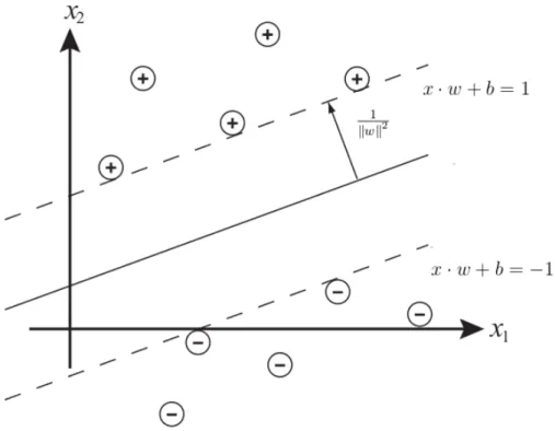
Figure 2.2: Linearly separable data, showing the hyperplane decision boundary and the separating margin
2.2 Support vector machine
Support vector machine (SVM) is a machine learning technique for data classication. A classication task usually involves separating data into training and testing sets. Each object in the training set contains one class label and several features. The goal of SVM is to produce a model that is capable of predicting the class labels of the test data given only the test data features.
The input for SVM is provided as a set of training samples xi ∈ Rn and corre-sponding classesyi ∈ {1,−1}n, where n is the size of the training set. The input space is divided into decision regions, and the boundaries that separate regions are called decision boundaries.
2.2.1 Linearly separable case
Let's assume that the data is linearly separable, meaning that we can draw a hyperplane between points belonging to dierent classes. This hyperplane can be described by
w·x+b = 0 wherew is normal to the hyperplane, b w
is the perpendicular distance from the hyperplane to the origin.
Points located closest to the separating hyperplane are called support vectors. The perpendicular distance between a point and the hyperplane is called margin:
• The functional margin uses the measure yi(xi·w+b) and is always positive for a correctly classied point.
hyperplane.
The margin of the hyperplane is the minimum geometric margin of all correctly classi-ed points. The aim of SVM is to orientate the separating hyperplane as far as possible from the closest members of both classes or, in other words, to maximize the margin.
SVM introduces a xed functional half-margin of 1, so the points from the training set can be described by the following equations:
xi·w+b≥1 foryi = 1
xi·w+b≤ −1 foryi =−1 These equations can be combined into:
yi(xi·w+b)−1≥0 ∀i
Planes, where support vectors lie, are called decision boundaries and can be de-scribed by:
x·w+b= 1
x·w+b=−1
The idea of nding the maximal margin hyperplane, while keeping the points clas-sied correctly, can be formalized in the following way:
min w,b 1 2 w 2 subject toyi(w·xi+b)≥1. (2.2) This problem is referred to as a primal problem. A Lagrangian function associated with 2.2 can be formulated as following:
L= 1 2 w 2 + N X i=1 αi(1−yi(w·xi+b)) (2.3)
Optimization problem 2.2 can be converted into the dual form, which is a con-vex quadratic problem where the objective function Φ depends solely on Lagrangian
multipliersαi: min α Φ(α) =minα 1 2 N X i=1 N X j=1 yiyj(xi·xj)αiαj − N X i=1 αi subject to αi ≥0 N X i=1 yiαi = 0
The dual form represents the minimum bound of the Lagrangian 2.3, in case of the strong duality, the optimal values of the primal problem and dual problem are equal.
Figure 2.3: Non-separable data showing misclassication error ξ
2.2.2 Linearly non-separable case
Since not all data sets are linearly separable, a modication to original statement 2.2 was introduced[5], which allows, but penalizes, error classications, i.e inability of the elements to reach the correct margin. Modication is done by adding slack variablesξ
that permit margin failure:
min w,b,ξ 1 2 w 2 +C N X i=1 ξi subject to yi(w·xi+b)≥1−ξi.
Here, C is a parameter allowing to balance between margin maximization and
minimization of classication error.
Using the Lagrangian, optimization problem can be presented in dual form as fol-lowing: min α Φ(α) =minα 1 2 N X i=1 N X j=1 yiyj(xi·xj)αiαj − N X i=1 αi subject to 0≤αi ≤C N X i=1 yiαi = 0
Lagrange multipliers extend the unconstrained rst-order condition to the case of equality constraints. To add inequality constraints, Karush-Kuhn-Tucker (KKT) con-ditions must be applied. KKT concon-ditions are necessary concon-ditions for the local mini-mum solutions. If pointxi is an optimal point, then the following KKT conditions are satised:
0< αi < C =⇒yi(xi·w+b) = 1
αi =C =⇒yi(xi·w+b)≤1
In the case when decision function is not the linear function, the input data has to be mapped to some other space (possibly, with innite dimensions), using a mapping
Ψ : X → H. Since the data appears in the training problem only in the form of
dot products xi·xj, explicit knowledge of Ψis not required, all we need is a function that would represent the dot product of the mapped input points Ψ(xi)·Ψ(xj). Such function is called a kernel function:
K(xi, xj) =
Ψ(xi)·Ψ(xj)
Replacing the dot product by kernel function, we obtain the output of a non-linear SVM:
N
X
j=1
yjαjK(xj, xi) +b
It is possible to extend SVM binary classication to the more general case of n
classes, by repeatedly applying binary classications. Binary classiers are trained for each pair of classes. Majority voting of the classiers is used to determine the class of the test sample.
Chapter 3
Optimization
Optimization deals with nding the optimum point, where the objective function reaches its minimum or maximum value. Optimization problem can be of two types - constrained and unconstrained. If the unconstrained optimization problem requires to nd an optimum point, then with constrained optimization several additional con-ditions have to be satised.
Optimization approaches have been widely used in machine learning due to their attractive theoretical properties[16]. Since the mid-1990s, there has been extensive research on algorithms for SVMs, and a variety of techniques have been proposed.
The optimization techniques for SVM can be divided into three main groups:
• decomposition methods the idea behind this method is to chunk the variables
from the QP into subsets and then solve the QP on each of the subset.
• interior point methods reformulates the problem with logarithmic barrier
func-tions instead of inequalities
• gradient-based methods use the properties of the gradient to nd the location
of optimal point
The following chapter gives overview of some of these techniques.
3.1 Sequential minimal optimization
Sequential minimal optimization (SMO) is an algorithm for solving SVM optimiza-tion problem analytically and uses Osuna's theorem[9] to ensure convergence. It was proposed by John C. Platt in 1998. SMO is one of the decomposition methods, that takes the smallest possible subset of two Lagrange multipliers and optimizes them an-alytically. Its runtime is linear in the number of training examples, in the worst case beingΩ(n2d), which is a big improvement over older methods that scale like n3, but is
obviously infeasible on large datasets.
Platt changes the denition of the hyperplane, denoting is as following:
u=w·x−b (3.1)
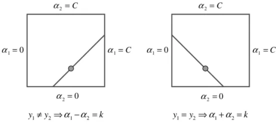
Figure 3.1: The two Lagrange multipliers must fulll all of the constraints of the full problem. The inequality constraints cause the Lagrange multipliers to lie in the box. The linear equality constraint causes them to lie on a diagonal line[12].
min α Φ(α) = minα 1 2 N X i=1 N X j=1 yiyjK(xi·xj)αiαj − N X i=1 αi subject to 0≤αi ≤C N X i=1 yiαi = 0
To ensure that the kernel is actually a dot product in the feature space, the kernel functionK must obey Mercer's conditions:
ˆ ˆ
K(x, y)g(x)g(y)dxdy≥0 (3.2)
At every step, SMO takes the smallest possible set of Lagrange multipliers (in standard case, two), nds an optimal value for them and updates SVM to reect this optimization. The numerical QP optimization is avoided since optimization of multipliers is done analytically. Additional advantage of SMO lies in a little resource usage, since no matrix storage is required[12].
In order to optimize two Lagrange multipliers, SMO computes the constraints on chosen multipliers and then solves the constrained minimum. Because only two multi-pliers are used, the constrains can be displayed in two dimensions3.1.
The algorithm rst computes the second Lagrange multiplier α2and nds the ends
of the corresponding diagonal segment. If the classesy1 and y2 are not equal, then the
following bounds apply toα2:
L=max(0, α2−α1)
H =min(C, C +α2−α1)
L=max(0, α2+α1−C)
H =min(C, α2+α1)
The second derivative along the diagonal line is:
η=K(x1, x1) +K(x2, x2)−2K(x1, x2)
Due to limitation 3.2 derivative of the objective function will always be positive denite and η will always be positive, and minimum along the diagonal line can be
computed:
αnew2 =α2+
y2(E1−E2)
η ,
whereEi =ui−yi is the error on the ith training entry.
At the next step, the constrained minimum is computed by clipping the constrained minimum to the ends of the diagonal segment:
αclipped2 = H if αnew 2 ≥H αnew 2 if L < αnew2 < H L if αnew 2 ≤L
The value of the rst Lagrange multiplier α1 is computed from the obtainedα2:
αnew1 =α1+y1y2(α2−αclipped2 )
To ensure that KKT conditions are fullled for both optimized multipliers, a thresh-old is recomputed at each step:
b1 = E1+y1(αnew1 −α1)K(x1, x1) +y2(α2clipped−α2)K(x1, x2) +b
b2 = E2+y1(αnew1 −α1)K(x1, x2) +y2(α2clipped−α2)K(x2, x2) +b
SMO chooses the threshold to be halfway in between b1 and b2.
In order to speed convergence, SMO uses heuristics to choose which two Lagrange multipliers should be optimized at the current iteration. There are two separate heuris-tics for each of the two Lagrange multipliers.
The rst Lagrange multiplier is chosen by iterating over the entire training data to nd the element that violates the KKT conditions. The second multiplier is chosen among the non-bound examples that also violate KKT conditions. The SMO algorithm terminates if the entire training set obeys the KKT conditions.
3.2 Interior point method
The early attempts to apply IPMs in the support vector machine training context were successful enough to generate further interest towards new developments. IPM is capable to reduce the cost of linear algebra operations due to the problem's special structure.
IPM solves the convex quadratic programming (QP) problem, which can be represented in the primal and dual forms in the following way:
Primal Dual min cTx+ 12xTQx subject to Ax=b x≥0 maxbTy− 1 2x TQx subject to ATy+s−Qx=c s≥0
whereA∈Rm×n has full row rank m≤n, Q∈
Rn×n is a positive semidenite matrix,
x, s, c∈Rn and y, b∈ Rm.
Using Lagrangian duality theory, the rst-order optimality conditions can be writ-ten as:
Ax= b ATy+s−Qx= c XSe= 0 (x, s)≥ 0,
where X and S are diagonal matrices in Rn×n with elements of vector x and s spread across the diagonal, respectively, and e ∈ Rn is the vector of ones. The third equation, XSe = 0, is called the complementarity condition and is often a source of
diculty when solving optimization problems.
Interior-point methods replace XSe = 0 with XSe = µ, where the parameter µ
is driven to zero. This operation removes the need to partition inequality constraints into active and inactive: the algorithm gradually reduces µ, and the partition of
vec-tors x and s into zero and nonzero elements is gradually revealed as the algorithm
progresses[16].
The best IPM algorithm known to date nds the ε-accurate solution of an LP or
convex QP problem inO(√nlog(1ε)) iterations [13]. However, one iteration of an IPM
may be costly. IPM involves the complete matrix to compute the Newton direction based on rst-order optimality conditions, and this operation may be expensive due to nontrivial sparsity patterns in the matrix.
The derivation of an interior-point method for optimization relies on three basic ideas:
1. Inequality constraints are replaced by logarithmic barrier functions
2. Duality theory is applied to barrier subproblems to derive the rst-order opti-mality conditions which take the form of a system of nonlinear equations
3. The system of nonlinear equations is solved by Newton's method
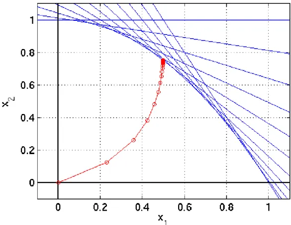
Implementation of IPMs deals with reducing the barrier term from a large initial value to small values needed to weaken the barrier and to allow the algorithm to approach an optimal solution[16]. In the linear programming case, the optimal solution lies on the boundary of the feasible region and many components of vectorx are zero (3.2).
Interior-point methods have proved eective on convex quadratic programs. How-ever, the density and the size of the kernel matrix make it dicult to achieve e-ciency. To get around this diculty a method to replace the Hessian with a low-rank approximation (of the formV VT, where V ∈ Rm×r for r m) is proposed. This ap-proach works well on problems of moderate scale, but may be too expensive for larger problems[16].
Figure 3.2: Trajectory of optimality conditions as µranges from innity down to zero
3.3 Gradient methods
Gradient methods are based on gradient information. They can be grouped into two classes, rst-order and second-order methods. First-order methods are based on the linear approximation of the Taylor series, and entail the gradient g. Second-order
methods, or Newton methods, are based on the quadratic approximation of the Taylor series. They entail the gradientg as well as the Hessian H. The drawback of a
second-order method is that the Hessian for a training set with n features is a n×n matrix.
When n is large, computing or storing this matrix can be impossible.
One of the rst-order methods is a gradient descent, also known as steepest descent method (algorithm 3.1). This method uses the fact that the gradient∇f of a function
points in the direction of greatest increase, meaning that−∇f points in the direction
Algorithm 3.1 Gradient descent
1. Input xo and initialize the tolerance ε. Set k = 0 2. Calculate gradient gk and set dk=−gk
3. Using line search, nd αk, the value of α that minimizes f(xk+αdk) 4. Set xk+1 =xk+αkdk and calculate fk+1 =f(xk+1)
5. If αkdk
< ε, then output x? = xk+1 and f(x?) = fk+1, and stop. Otherwise,
of greatest decrease.
In gradient descent, the gradient is computed using the entire training set. A simple alteration of this is to nd the gradient with respect to a single randomly chosen example. This technique is called stochastic gradient descent (SGD). By using only a single example an approximation to the true gradient is obtained, therefore, there is no guarantee of movement in the direction of the greatest descent. Still, there are at least two important reasons why stochastic gradient descent is used for SVM training:
• it is signicantly quicker than gradient descent when data set is large
• stochastic gradient descent minimizes the generalization error quicker than
gra-dient descent
While gradient based methods are known to exhibit slow convergence rates, the com-putational demands imposed by large scale classication and regression problems of high dimension feature space, renewed the interest in gradient methods[16].
Chapter 4
Parallelization
One of SVM algorithm's disadvantages is the large memory requirement and compu-tation time required to deal with large datasets. The reason is the core problem of an SVM - a quadratic programming problem (QP) that separates support vectors from the rest of the training data. General-purposed QP solvers tend to scale with the cube of the number of training vectorsO(n3)[10]. To speed up the process of training SVM,
parallel methods have been proposed and have proved to be ecient.
4.1 Parallel SMO
Sequential minimal optimization algorithm has proved to be inecient due to usage of a single threshold value. A modication of SMO was proposed introducing two threshold variables blow and bup that are used to check the solution for optimality[8]. To speed up optimality verication,indexes of Lagrange multipliers i ∈ 1...n are divided into
four subsets based on the value of Lagrange multiplier and corresponding class label. At each step the worst pair of multipliers is chosen for optimization. These modied algorithms perform signicantly faster than the original SMO[15].
It was noted that the most time consuming operation of SMO is the update of
ui array (see equation3.1), that holds the output of SVM for the ith training sample. To decrease the computation time, a parallel implementation of SMO was proposed[2] that would calculateu in parallel.
In the parallel implementation of SMO, the input data is divided into a number of subsets, based on the amount of nodes in use. Each node gets its own set of the Lagrange multipliers to optimize.
The program terminates, when duality gap gets close to zero. Duality gap is a variable, holding the dierence between the primal and dual forms of the objective function. If it reduces to zero, the optimum is reached.
DualityGap= N X i=0 αiyiξi + n X i=0 εi, where εi = ( C·max(0, b−ξi) yi = 1 C·max(0,−b+ξi) yi =−1
The global instance of the duality gap is introduced, shared by all nodes, and equal to the sum of the DualityGap of the all processors.
Figure 4.1: Schematic of a binary Cascade architecture. TD: Training data, SVi:
Support vectors produced by optimization i.[7]
4.2 Cascade SVM
Another approach to parallelization of SVM has been proposed by splitting the problem into smaller subsets and training a network to assign samples to dierent subsets.
It has been proved that eliminating non-support vectors early from the optimization can speed-up SVM eciently[7].A ltering process for the elimination can be done in parallel.
The problem is initialized with a number of independent, smaller optimizations. Then, the partial results are combined in a hierarchical fashion. In the architecture, shown on Figure 4.2, sets of support vectors from two SVMs are combined and the optimization process continues with search for the support vectors in each of the com-bined subsets. The process ends when only one set of the vectors is left. Often it is enough to pass the cascade only once to get satisfactory accuracy, but if the global optimum has to be reached, the result of the last layer is sent back to the rst layer. Each of the SVMs in the rst layer receives all the support vectors of the last layer as inputs and then tests if any of them have to be incorporated into the optimization. If this is not the case for all SVMs of the input layer, then the global optimum is reached, otherwise another pass through the network is made.
One of the main advantages of the Cascade architecture is that it requires far less memory than a single SVM, because the size of the kernel matrix scales with the square of the active set.
4.3 PSVM
PSVM is a parallel approximate implementation of SVM that aims to reduce both loading and computation time. Training set is loaded into several machines in a cyclic
fashion, and a parallel row-based Incomplete Cholesky Factorization (ICF) is then applied on the data. At the end of ICF, each machine stores only a part of factorized matrix. PSVM then performs parallel IPM to solve quadratic optimization problem.
PSVM devises parallel row-based ICF (PICF) at its initial step, which loads training instances onto parallel machines and performs factorization simultaneously on these machines. The size of kernel matrix is reduced through factorization, which helps to reduce used space to O(np/m), wherep/m is much smaller than n.
ICF can approximateQ∈Rn×nby smaller matrixH ∈
Rn×p, pn, i.eQ≈HHT. Row-based parallel ICF (PICF) works as follows. Let vector v be the diagonal of Q
and suppose the pivots (the largest diagonal values) are{i1, .., ik}, the kth iteration of ICF computes three equations:
H(ik, k) = p v(ik) H(Jk, k) = Q(Jk, k)− Pk−1 j=1H(Jk, j)H(ik, j) H(ik, k) v(Jk) = v(Jk)−H(Jk, k)2,
where Jk denotes the complement of {i1, .., ik}. The algorithm iterates until the approximation of Q by HkHkT is satisfactory, or the predicted maximum of iterations (or, the desired rank of the ICF matrix)p is reached.
Row-based approach starts by initializing variables and loading training data to m machines in a cyclic way. In each iteration k, ve tasks are performed:
1. A pivot, which is the largest value in the diagonal v of matrix Q, is found in parallel
2. Machines that hold the pivot are marked as master
3. On the master, PICF calculates H(ij, k)according to H(ik, k) =
p
v(ik)
4. The pivot instance xik and the pivot rowH(ik,:)are broadcasted by the master
node 5. H(Jk, k) = Q(Jk,k)− Pk−1 j=1H(Jk,j)H(ik,j) H(ik,k) and v(Jk) =v(Jk)−H(Jk, k) 2 are computed in parallel manner
At the end of the algorithm,H is distributed onm machines, and the system is ready
for parallel IPM to be applied.
PICF has three advantages: parallel memory use, parallel computations and low communication overhead.[4]
Parallel IPM minimizes both storage and communication cost by distributing the data:
1. Distributed matrix data. At the end of PICF matrix H is divided between the nodes.
2. Distribute n×1 vector data. All n×1 vectors are distributed in a round-robin
3. Replicated global scalar data. Every machine caches a copy of global data in-cluding v,t,n and 4v. Whenever scalar is changed, a broadcast is required to
maintain global consistency.
When the IPM iteration stops, we have the value of αand the classication function: f(x) =
N
X
i=1
αiyik(si, x) +b
HereN is the number of support vectors and si are support vectors.
In order to complete classication function,b must be computed. An average value
of b can be computed in parallel using mapReduce[6].
4.4 P-packSVM
P-packSVM is based on simple stochastic gradient descent (SGD) based algorithm that directly optimizes primal objectivef(w) = σ2kwk22+ m1 Pm
i=1max{0.1−yihw, φ(xi)i}. At each iteration, a single sample from the training set is picked at random to ap-proximatel(w) = m1 Pm
i=1max{0.1−yihw, φ(xi)i}, and then the gradient is calculated and the predictor w is updated accordingly. Parallelized is done with the help of a distributed hash table and a special packing strategy. SGD algorithms have huge com-munication cost, which is non-trivially reduced by packing strategy that also allows a sub-linear speed-up.
At each iteration t ∈ {1, ..., T}, a random example (xi(t), yi(t)) ∈ ψ is picked and the empirical loss l(w) = m1 Pm
i=1max{0.1−yihw, φ(xi)i} and the objective f(w) = σ 2 kwk 2 2+ 1 m Pm
i=1max{0.1−yihw, φ(xi)i} are approximated in a following manner:
l(w)≈lt(w) :=max{0.1−yi(t)· w, φ(xi(t)) } f(w)≈ft(w) := σ 2kwk 2 2+lt(w)
In iteration t the predictor is modied:
w←w− 1
σt∇ft(w)
The sub-gradient can be written down explicitly:
∇ft = ( σw yi(t)· w, φ(xi(t)) ≥1 σw−yi(t)φ(xi(t)) yi(t)· w, φ(xi(t)) <1
At each update of w, a projection is applied to make w closer to the optimum:
w←min{1,1/
√
σ
kwk22 }w
There are two main characteristics that have to be considered when applying parallel paradigm:
• Merit. A single iteration can be parallelized. The calculation of hv, φ(x)ican be
• Defect. The mass communication will slow down the parallel program.
Taking these characteristics into consideration, a distributed hash table to develop merit is proposed, and a packaging strategy is used to overcome the defect.
Distributed hash table
Entries in H are averagely divided to all the processors. Suppose theithprocessor saves a subset
Hi ={(xi,j, βi,j)}
|Hi|
j=1 ⊂H to represent vi =Pjβi,jφ(xi,j)
The calculation of inner producthv, φ(x)i can be distributed to all the processors,
by each calculation hvi, φ(x)i=
P
jβi,jK(xi,j, x) and sum-up via inter-processor com-munications.
All the processors check whether the given key x exists in the local hash table Hi.
If any of the processors nds the key, it simply updates the value and informs other processors of the existence of the key.
Packing strategy
Several iterationsr ∈N are packed into a single one, and thus the number of
commu-nications is reduced by a factor ofO(r)[20]. The total bits in communication will not
be reduced.
Letwt, xt, yt denote the predictor w and the random sample (xt, yt) in the tth iter-ation.
Packing algorithm for r consecutive iterations t,...,t+r-1 is summarized as follows: 1. Calculateyi0 =hwt, φ(xt)i for i=t...t+r−1
2. CalculateK(xi, xj) for t≤i < j ≤t+r−1
3. Iteratei through t tot+r−1and process the ith iteration as before. Whenever
iterationiis nishedai, bi can be calculated andy
0
i+1, ..., y
0
t+r−1are updated oine
(without communication): 4. yi0+j ←αiy
0
i+j+biK(xi+j, xi)
5. The distributed hash table H is updated after all r iterations nish, by
commu-nicating to conrm the existing entries, and then add new entries to the least occupied processor.
Chapter 5
Performance tests
To make sure that parallelization does increase the performance speed, it is required to conduct some experiments on the data of dierent size and density. It must be noted, that performance is not the only parameter that should be taken into consideration -the accuracy of class prediction should not decrease. To test -the algorithms, described above, we used several datasets[3] that vary by data size and the number of features of the input vectors.
5.1 Setup
For the experiments, we chose the following algorithms:
• LIBSVM
• PSVM • SVMLight
The algorithms chosen use dierent type of solvers for the optimization problem, which makes it possible to compare the methods described in chapter 3. All algorithms were fed the same training data, characteristics of which can be observed in Table 5.1.
5.2 Results
The results obtained during the experiments, can be observed in tables 5.2 and 5.3. The dataset name is specied in the column, and the row denotes SVM implementation. Each cell contains training time in seconds.
As we can see from the table 5.2, LIBSVM runs even faster than PSVM on the data sets with a relatively small amount of features. PSVM, however, proves to be the
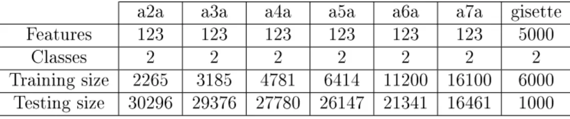
a2a a3a a4a a5a a6a a7a gisette
Features 123 123 123 123 123 123 5000
Classes 2 2 2 2 2 2 2
Training size 2265 3185 4781 6414 11200 16100 6000
Testing size 30296 29376 27780 26147 21341 16461 1000
a2a a3a a4a a5a a6a a7a gisette libSVM 0.283 0.422 1.287 1.987 6.4 13.071 279.406 SVMLight 0.530 0.972 2.367 4.267 13.645 28.714 408.214 PSVM nodes 1 2.039 6.029 21.250 55.337 401.784 1924.519 105.108 2 1.205 3.583 12.361 31.548 499.043 823.182 64.907 4 1.125 3.557 12.145 29.676 234.812 499.208 63.774 8 0.823 1.8 7.863 17.296 131.847 429.786 49.002 16 0.906 1.699 4.792 11.729 83.428 282.933 30.782 32 2.518 4.503 10.142 65.650 200.362 24.298 64 4.802 10.543 50.296 159.619 20.617
Table 5.2: Training Performance SVM implementations on dierent datasets.
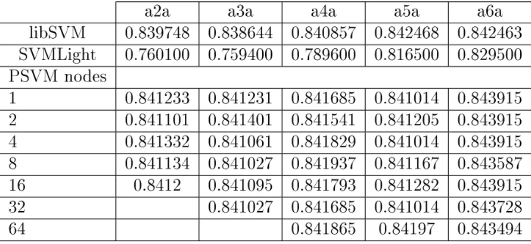
a2a a3a a4a a5a a6a
libSVM 0.839748 0.838644 0.840857 0.842468 0.842463 SVMLight 0.760100 0.759400 0.789600 0.816500 0.829500 PSVM nodes 1 0.841233 0.841231 0.841685 0.841014 0.843915 2 0.841101 0.841401 0.841541 0.841205 0.843915 4 0.841332 0.841061 0.841829 0.841014 0.843915 8 0.841134 0.841027 0.841937 0.841167 0.843587 16 0.8412 0.841095 0.841793 0.841282 0.843915 32 0.841027 0.841685 0.841014 0.843728 64 0.841865 0.84197 0.843494
Table 5.3: Prediction accuracy
most ecient when the input vector has a large number of features, since it stores the feature vectors in parallel. That can be easily explain by the nature of the QP problem solvers used in both implementations. LIBSVM uses SMO and does not store the kernel function values, so they have to be calculated on demand, while PSVM stores the kernel matrix in parallel, and kernel function for each point has to be calculated only once. As the number of features grows, the calculation of kernel function becomes more and more time and resource consuming.
The accuracy of the class prediction for all tested implementations does not vary signicantly, and is not dependent on the size of the dataset. It can be easily explained by the fact that all the SVM solvers look for the global optimal point of the same objective function and the result should not depend on the way optimization problem is solved.
Chapter 6
Support Vector Clustering
Support vector clustering (SVC) is a non-parametric clustering algorithm based on the support vector approach. Support vector clustering algorithm data points are mapped from data space to a high dimensional feature space using a Gaussian kernel. The sphere is then mapped back to data space, where it forms a set of contours that enclose the data points and can be interpreted as cluster boundaries. Points enclosed by each separate contour belong to the same cluster.
SVC algorithm is known to have two main bottlenecks - expensive computation and poor labeling performance. To overcome these disadvantages, an improved version of algorithm was proposed. Parallel algorithms, used for training SVM to improve the performance of SVC, are applied to SVC for performance improvement.
6.1 Support Vector Clustering
Support vector clustering is a non-parametric clustering algorithm based on the sup-port vector approach. The mathematical formulation of the SVC algorithm can be summarized as follows: assume a dataset containing N points {x1, x2, .., xN},xi ∈ Rd, where d is the dimension of the data space. A nonlinear mapping function Ψ is used
to map the data set into a high-dimensional feature space such that the radius of the sphere, R, enclosing all the data points is as small as possible. Such an objective can be formulated by the following optimization problem:
minR2 +CX j ξj subject toΨ(xj)−a 2 ≤R2+ξj∀j, (6.1) where
·is the Euclidean norm, a is the center of the sphere,ξj are slack variables
that loosen the constraints to allow some data points to lie outside the sphere, C is a
constant, andCP
ξj is a penalty term. To solve the optimization problem in 6.1, it is convenient to introduce the Lagrangian function:
L(R, a, ξj, αj, µj) = R2− X j (R2+ξj − Ψ(xj)−a 2 )αj− X ξjµj+C X ξj, (6.2) where αj ≥ 0 and µj ≥ 0 are the Lagrange multipliers. With 6.2, we can derive the following conditions by the Lagrange theorem and the Karush-Kuhn-Tucker (KKT) complementarity[5]:
ξjµj = 0, (6.3) (R2+ξj− Ψ(xj)−a 2 )αj = 0 (6.4)
According to 6.3 and 6.4, we can classify each data point into 1. an internal point
2. an external point
3. a boundary point in the feature space
Point xj is classied as an internal point if αj = 0. When 0< αj < C, the data point
xj , is denoted as a support vector. Support vectors lying on the surface of the feature-space sphere are called boundary points. These support vectors are used to describe the cluster contour in the input space. Whenαj =C, the data points located outside the feature space are dened as the external points or bounded support vectors.
Using the above conditions, 6.1 can be turned into the Wolfe dual optimization problem with only variablesαj:
maxX j Ψ(xj)2αj− X i,j αiαjΨ(xi)·Ψ(xj) subject to 0≤αj ≤C X j αj = 1 ∀j, (6.5)
where the dot product of(Ψ(xi)·Ψ(xj))represents the Mercer kernel K(xi, xj). Gaus-sian functions are selected as kernels, i.e., K(xi, xj) = exp(−q
xi −xj 2 ). For any
point x in the data space, the distance of its image in the feature space from the center of the sphere is described by
R2(x) =Ψ(x)−a 2 =K(x, x)−2X j αjK(xj, x) + X i,j αiαjK(xi, xj) (6.6) The radius R of the sphere can be obtained by
R={R(xi)|xi is a support vector}. (6.7) The average of the above set is used as the radiusR. The support vectors, bounded
support vectors, and the other points are located on the cluster boundaries, the outside of the boundaries, and the inside of the boundaries, respectively.
There are two important parameters in SVC algorithm: q and C. The value of q
governs the number of clusters and the tightness of the cluster boundaries, while the value of C determines the existence of outliers during the clustering process.
The cluster description does not dierentiate points that belong to dierent clusters. If there are two data points, xi and xj , that belong to the same cluster in the input space, one can check if the line segment between them always lies within the high dimensional sphere. Checking the line segment is implemented by sampling a number of points on the segment. Two data points, xi and xj , satisfying the above condition
are dened as the components of the same cluster. An adjacency matrix A is dened
to identify the components of a cluster. The components of A, aij , between pairs of pointsxi and xj, are dened as follows:
aij =
(
1, if all y on the line segment connecting xiand xj, R(y)≤R
0, otherwise (6.8)
The values of aij can be obtained by sampling a number of points from the line segment connecting xi and xj . In the matrix A, if aij = 1 that means xi and xj belong to the same cluster; otherwise, they are in dierent clusters. A positive decision function guarantees thatxi andxj are part of the same cluster. In case of the negative decision function, it is still possible that points belong to the same cluster, but are recognized as the points from dierent contours, which is likely to occur in the case of complex contours. In general, the cluster labeling step that checks the connectivity for each pair of samples is more time-consuming than the SVC training step. The time complexity of this procedure is O(lN2), where l is the number of samples on the line
segment[19].
6.2 Improved support vector clustering (iSVC)
An improved SVC algorithm, iSVC, address two known bottlenecks of SVC (costly computation and labeling) simultaneously[11]. iSVC includes a reduction strategy that can help to develop clustering model on a qualied subset. Reduction strategy aims to increase eciency. It is based on the Schrödinger equation and extracts a desired subset based on which the clustering model is formulated.
iSVC labels data according to the geometric properties of the feature space. Firstly it handles arbitrary-shaped clusters through its boundary-based clustering model. Sec-ondly it deals with structured data by employing Kernel function.
6.2.1 Optimization piece of iSVC
In iSVC's optimization piece, reduction strategy is performed on the whole dataset, and then the modied objective is optimized on the subset.
Reduction strategy is based on the Schrödinger equation that describes the law of energy conservation of a particle, written as follows:
Hψ(x)≡(−σ
2
2 ∇
2+P(x))ψ(x) =eψ(x),
where e is the energy, P(x) the Schrödinger potential, r the Laplacian, and s the
variance parameter. c(x) expresses the state of a quantum system, so c(x) can be
explained as the wave function of particle. When applied in machine learning,c(x)can
be considered a data probability distribution function, and its maxima is associated with cluster centers[11]. For the givenψ(x), P(x) is solved as follows:
P(x) = e+ σ
2
2ψ(x)∇
2
ψ(x)
From geometry meaning, minima ofP(x)tells cluster centers, so P(x)'s maximum
iSVC develops clustering model from a subset. Points located around cluster con-tours should be included in the subset. The subset should cover all clusters. Qualied subset is found by employing the Schrödinger equation to explore data position infor-mation.
P(x) values reveal data location: points with top P(x) values tend to be around cluster boundaries, while points with small P(x) values are usually located in cluster central zones. The reduction strategy has the following steps:
1. Sort {P(xi)} values in the descending order:{P(i)}, with P(i) ≥ P(i+1), where
P(i) =P(xi), i= 1, ..., N
2. Specify the interval length G of {P(i)} list to separate the list into L intervals
L=N/G:
{P(1)...P(G)},{P(G+1)...P(2G)}, ...,{P((L−1)G)...P(LG)}
1. In each interval, some data are sampled randomly at a certain ratio. For Jth interval,{P((J−1)G)...P(J G)} its sampling ratio is as follows:
ηJ =max{
1
J,
1
G}
G balances the clustering quality and the cost. The higher the G, the bigger the
subset size.
The reduction strategy reduces the optimization from the whole set to the subset.
6.2.2 The labeling piece of iSVC
iSVC introduces the new labeling approach, whose idea is to cluster support vectors rst, then construct a classier based on labeled support vectors. Finally, other data is labeled using the classier.
1. Create anity matrix H with respect to support vectors according to Gaussian Kernel: Hij =k(vi, vj) with vi and vjbeing support vectors.
2. Normalize H intoH0: H0 = Λ−1/2HΛ−1/2, whereΛ =diag(P
jHij)
3. Do eigenvalue decomposition on H0, and take top g eigenvectors as columns to
form matrix H00.
4. Perform K-means on rows of H00; the cluster number is initialized as g. g is
specied by the number of eigenvalues that are larger than 1. 5. Label vi as the ith row's cluster membership.
Algorithm 6.1 Parallel SVC pseudocode p := number of p r o c e s s o r s
subProblems := divideIntoSubproblems ( t r a i n i n g S e t , p) while ( not optimumIsReached ( ) ) {
subProblems [ i ] . eliminateNonSV ( )
merge ( subProblems [ i ] , subProblems [ i +1]) } R := c a l c u l a t e R a d i u s ( ) each ( subProblems ){ calculateAdajencyMatrix ( ) }
6.3 Parallel SVC
The experiments conducted on parallel implementations of SVM showed that paral-lelization can eciently increase the performance of the algorithm without losing the accuracy of class prediction. It was proposed that it is possible to apply the paral-lelization techniques to SVC algorithm and a parallel SVC was proposed (Algorithm 6.1).
First of all, we are seeking to reduce the size of the original training data. Since only support vectors are required to calculate the radius of the enclosing sphere, it was decided to apply the ltering technique used in CascadeSVM, which would eliminate non-support vectors in parallel.
Calculation of adjacency matrix, which is the most time-consuming part of SVC algorithm, can also be done in parallel. Input vectors are divided into subsets and then are evenly distributed among the nodes. The accuracy of cluster prediction does not change and remains the same as the one in the non-parallel implementation, since calculation of the adjacency matrix in parallel does not change its contents.
Chapter 7
Summary
Support vector machine is a powerful machine learning technique used for binary clas-sication of data. The algorithm of SVM separates objects of one class from another by solving the quadratic programming problem. For that reason, SVM's training takes a lot of computation time and consumes a large amount of memory.
To speed up the SVM algorithm, several parallel implementations were proposed, using dierent optimization techniques and approaches to parallelization. We looked at some parallel algorithms for SVM, such as PSVM, pPackSVM and CascadeSVM. Techniques for distributed computing proposed in these algorithms can be summarized as follows:
• Distributed storage of data. Kernel matrix and training data are divided into
subsets and each subset is stored on the separate machine.
• Sub-problems are solved in parallel. QP problem is solved for each of the training
data subset in the separate node.
• Training data is reduced by parallel preprocessing. Training data is ltered and
non-support vectors are eliminated.
• Reduced number of communications between nodes. Each node is sending
re-sults of several iterations at once, which reduces the time required for network communication.
Experimental results obtained has shown, that parallelization of SVM can considerably decrease the computation time and the amount of memory used by each machine. The prediction accuracy of the parallel algorithms is as high as the accuracy of the iterative implementations.
The given thesis also provided a description of SVC, a clustering algorithm based on SVM, and proposed several ways to increase its performance and calculation speed of the adjacency matrix. We proposed a parallel algorithm for SV that signicantly reduces the computation time, while the assignation of points into the clusters remains the same.
The parallel approach to solving the optimization problem and assigning the data points to clusters reduces the computation speed and makes the SVC algorithm ap-plicable for large datasets. In the future, a parallel SVC might be applied to real life problems and might prove to be both ecient and accurate clustering algorithm, which will increase the popularity of SVC in the scientic community.
Resümee
Vektormasinate paralleeliseerimine
Magistritöö Olga Agen
Tugivektormasin (Support Vector Machine) on masinõppe meetod, mida kasutakse andmete klassitseerimiseks. Binaarse klassikatsiooni probleem seisneb sellise funkt-siooni või mudel leidmisel, mis oskaks ennustada, mis klassi etteantud punktxi kuulub. Mudeli treenimiseks kasutatakse treeningandmeid.
Treeningandmed on esitatud hulgast{(xi, yi)|xi ∈X, yi ∈ {1,−1}, i= 1, ..., n}, kus X on punktide hulk ning yi on klass, millesse antud punkt xi kuulub.
Sisendpunktidxi tavaliselt teisendatakse omaduste ruumi H kasutades tuuma funk-tsiooni ϕ : X → H, ning mudel õpitakse teisendatud andmete peal.
Õppimisprotses-sis leitakse optimaalset hüpertasandit, mis eraldab erinevasse klassidesse kuuluvaid punkte. Leitud hüpertasand on optimaalne siis, kui mõlema klassi punktide kaugus tasandist on maksimaalne. Kauguse maksimiseerimist on võimalik väljendada järgmise optimeerimisprobleemi kaudu: min w,b 1 2 w 2 tingimusel, etyi(w·xi−b)≥1,∀i
Optimeerimisprobleemi lahendamiseks on mitu algoritmi. Meie vaatame nendest ainult mõnda, seal hulgas:
• Järjestikune minimaalne optimeerimine (Sequential Minimal Optimization) • Sisepunkti meetod (Interior point method)
Tugivektormasinal põhineb klasterdamisalgoritm, mis otsib omaduste ruumis mini-maalse raadiusega sfääri, mis ümbritsed teisendatud sisendpunkte. Seda sfääri kir-jeldab järgmine võrrand:
ϕ(xi)−a 2 ≤R2 ∀j,
kus a on sfääri keskpunkt.
Selleks, et jaotada punkte erinevate klastrite vahel, kasutatakse punktide vahelist kaugust d(x). Punktid kuuluvad samasse klassi kui nende vaheline lõik on täielikult sfääri sees, ehk iga lõigu punkti y puhul kehtib d(y)>R, kus R on sfääri raadius.
Oma töös võrdlesime iteratiivsed ja paralleelseid tugivektormasina algoritmide im-plementatsioone. Uurimise käigus avastasime et paralleelsed algoritmid, nagu oligi oodatud, töötavad palju kiiremini kui iteratiivsed, seejuures valesti klassitseeritud punktide arv ei suurene.
Lisaks implementeerisime klasterdamisalgoritmi kasutades paralleliseerimise viise, mida kasutatakse klassitseerimisprobleemi lahendamiseks. Paralleelne
imelementat-sioon näitas, et klasterdamisalgoritmi jaoks on võimalik kasutada samu paralleliseer-imismeetodeid, mida on kasutatud vektormasinate puhul.
Bibliography
[1] Asa Ben-Hur, David Horn, Hava T. Siegelmann, and Vladimir Vapnik. Support vector clustering. JOURNAL OF MACHINE LEARNING RESEARCH, 2:125 137, 2001.
[2] L. J. Cao, S. S. Keerthi, Chong-Jin J. Ong, J. Q. Zhang, Uvaraj Periyathamby, Xiu Ju J. Fu, and H. P. Lee. Parallel sequential minimal optimization for the training of support vector machines. IEEE transactions on neural networks / a publication of the IEEE Neural Networks Council, 17(4):10391049, July 2006. [3] Chih-Chung Chang and Chih-Jen Lin. Libsvm: A library for support vector
machines. ACM Trans. Intell. Syst. Technol., 2(3):27:127:27, May 2011.
[4] Edward Y. Chang, Kaihua Zhu, Hao Wang, Hongjie Bai, Jian Li, Zhihuan Qiu, and Hang Cui. Psvm: Parallelizing support vector machines on distributed computers. [5] Corinna Cortes and Vladimir Vapnik. Support-vector networks. In Machine
Learn-ing, pages 273297, 1995.
[6] Jerey Dean and Sanjay Ghemawat. Mapreduce: simplied data processing on large clusters. Commun. ACM, 51(1):107113, January 2008.
[7] Hans Peter Graf, Eric Cosatto, Leon Bottou, Igor Durdanovic, and Vladimir Vap-nik. Parallel support vector machines: The cascade svm. In In Advances in Neural Information Processing Systems, pages 521528. MIT Press, 2005.
[8] S. S. Keerthi, S. K. Shevade, C. Bhattacharyya, and K. R. K. Murthy. Im-provements to platt's smo algorithm for svm classier design. Neural Comput., 13(3):637649, March 2001.
[9] Edgar Osuna, Robert Freund, and Federico Girosi. An improved training algo-rithm for support vector machines. pages 276285. IEEE, 1997.
[10] Jian pei Zhang, Zhong-Wei Li, and Jing Yang. A parallel svm training algorithm on large-scale classication problems. In Machine Learning and Cybernetics, 2005. Proceedings of 2005 International Conference on, volume 3, pages 16371641 Vol. 3, 2005.
[11] Ling Ping, Zhou Chun-Guang, and Zhou Xu. Improved support vector clustering. Eng. Appl. Artif. Intell., 23(4):552559, June 2010.
[12] John C. Platt. Advances in kernel methods. chapter Fast training of support vector machines using sequential minimal optimization, pages 185208. MIT Press, Cambridge, MA, USA, 1999.
[13] James Renegar. A polynomial-time algorithm, based on newton's method, for linear programming. Mathematical Programming, 40(1-3):5993, 1988.
[14] Raul Rojas. Neural Networks - A Systematic Introduction. Springer-Verlag, Berlin, 1996.
[15] S. K. Shevade, S. S. Keerthi, C. Bhattacharyya, K. R. K. Murthy, and In Smola. Improvements to the smo algorithm for svm regression. IEEE Trans. Neural Netw, pages 11881193, 2000.
[16] Sebastian Nowozin Suvrit Sra and Stephen J. Wright. Optimization for Machine Learning. The MIT Press, 2012.
[17] V. N. Vapnik and A. Ya. Chervonenkis. Theory of Pattern Recognition [in Rus-sian]. Nauka, USSR, 1974.
[18] Vladimir Vapnik. Estimation of Dependences Based on Empirical Data: Springer Series in Statistics (Springer Series in Statistics). Springer-Verlag New York, Inc., Secaucus, NJ, USA, 1982.
[19] Jeen-Shing Wang and Jen-Chieh Chiang. An ecient data preprocessing procedure for support vector clustering. j-jucs, 15(4):705721, feb 2009.
[20] Zeyuan A. Zhu, Weizhu Chen, Gang Wang, Chenguang Zhu, and Zheng Chen. P-packSVM: Parallel primal gradient descent kernel SVM. In ICDM, 2009.
License
Non-exclusive licence to reproduce thesis and make thesis public
I, Olga Agen (14.09.1989),
1. herewith grant the University of Tartu a free permit (non-exclusive licence) to: (a) reproduce, for the purpose of preservation and making available to the
pub-lic, including for addition to the DSpace digital archives until expiry of the term of validity of the copyright, and
(b) make available to the public via the web environment of the University of Tartu, including via the DSpace digital archives until expiry of the term of validity of the copyright,
Parallelization of Support Vector Machines supervised by Oleg Batrashev and Artjom Lind,
2. I am aware of the fact that the author retains these rights.
3. I certify that granting the non-exclusive licence does not infringe the intellectual property rights or rights arising from the Personal Data Protection Act.

![Figure 4.1: Schematic of a binary Cascade architecture. TD: Training data, SV i : Support vectors produced by optimization i.[7]](https://thumb-us.123doks.com/thumbv2/123dok_us/475662.2556244/21.892.173.768.109.477/figure-schematic-cascade-architecture-training-support-produced-optimization.webp)