Multiple adaptive mechanisms for predictive models on streaming data.

models on streaming data

RASHID BAKIROV

A thesis submitted in partial fulfilment of the requirements of Bournemouth University for the degree of

Doctor of Philosophy

be made of the use of any material contained in, or derived from, this thesis.

Abstract

Making predictions on non-stationary streaming data remains a challenge in many application areas. Changes in data may cause a decrease in predictive accuracy, which in a streaming setting require a prompt response. In recent years many adaptive predictive models have been proposed for dealing with these issues. Most of these methods use more than one adaptive mechanism, deploying all of them at the same time at regular intervals or in some other fixed manner. How-ever, this manner is often determined in an ad-hoc way, as the effects of adaptive mechanisms are largely unexplored. This thesis therefore investigates different aspects of adaptation with multi-ple adaptive mechanisms with the aim to increase knowledge in the area, and propose heuristic approaches for more accurate adaptive predictive models. This is done by systematising and for-malising the “adaptive mechanism” notion, proposing a categorisation of adaptive mechanisms and a metric to measure their usefulness, comparing the results after deployment of different or-ders of adaptive mechanisms during the run of the predictive method, and suggesting techniques on how to select the most appropriate adaptive mechanisms.

The literature review suggests that during the prediction process, adaptive mechanisms are selected to be deployed in a certain order which is usually fixed beforehand at the design time of the algorithm. For this reason, it was investigated whether changing the selection method for the adaptive mechanisms significantly affects predictive accuracy and whether there are certain deployment orders which provide better results than others. Commonly used adaptive mechanism selection methods are then examined and new methods are proposed.

A novel regression ensemble method which uses several common adaptive mechanisms has been developed to be used as a vehicle for the experimentation. The predictive accuracy and be-haviour of adaptive mechanisms while predicting on different real world datasets from the process industry were analysed. Empirical results suggest that different selection of adaptive mechanisms result in significantly different performance. It has been found that while some adaptive mecha-nisms adapt the predictive model better than others, there is none which is the best at all times. Finally, flexible orders of adaptive mechanisms generated using the proposed selection techniques often result in significantly more accurate models than fixed orders commonly used in literature.

This thesis would not have been possible without those around me while I was writing it. Firstly I would like to thank to my supervisors, Bogdan Gabrys and Damien Fay for their continuous guidance, sharing of their knowledge and shaping me as a researcher. I also thank my former supervisor Indre ˇZliobait˙e for her input at the early stages of my PhD.

Many academics and peers have assisted the completion of the thesis in various ways during this time, for which I am very grateful. In particular, Petr Kadlec has provided me with his Matlab code. Marcin Budka, Manuel Mart´ın Salvador and Neil Vaughaun have given helpful feedback my thesis. Alejandro Tabas discussed some of the math with me. Akanda Ashraf, Bastian Fraune and Mohsen Amiribesheli shared their opinions about various plots and provided my wrists with exercise during daily table football games. Jan Walter Schroeder gave me general advices on writing the thesis.

I was blessed to have made many truly great friends during my PhD time, who made me feel at home in Bournemouth and have immensely contributed to my development as a person. For this, I deeply thank every single one of them - you know who you are. My special thanks goes to Diana for her constant support and encouragement. I would also like to thank Bomojam crew for the magical hours of music that we made together and lunchers for making our meals at the university something to look forward to. Also huge thanks to Kim, who has greatly contributed to my preparation for the viva.

Many people, including my former colleagues at University of Siegen, ABB Research Ger-many and PwC GerGer-many have helped and encouraged me on this path. Among others, I thank Klaus Hartmann, Chris Stich and Markus Anderle for their supervision and many recommenda-tion letters, and Seyed Eghbal Ghobadi for getting me interested in Machine Learning.

Staff at Bournemouth University has been most helpful during my PhD. In particular, I thank Naomi Bailey for the administrative assistance, Natalie Andrade and Malcolm Green for the help with finance related matters, and Shaun Bendall for the assistance with computing cluster.

I am grateful to my final viva examiners Emili Balaguer-Ballester and Vasile Palade, as well as transfer viva examiners Raian Ali and Hammadi Nait-Charif for their constructive and helpful comments on my theses. I thank anonymous reviewers, whose comments on my publications have improved my work and members of academia for the all their research that I was inspired by. I would also like to thank the creators of free software that have helped me greatly during writing of the thesis. These include LaTeX, TexStudio, briss, Excel2Latex, Putty and WinScp. My thanks also goes to the members of stackexchange.com whose questions and answers has solved many of Matlab and LaTeX riddles for me. I

Finally, I am ever thankful to my parents and my sister, who were always there for me during this time and in fact for whole my life.

Copyright statement . . . i

Abstract . . . ii

Acknowledgements . . . iii

Table of contents . . . iv

List of figures . . . vii

List of tables . . . ix

Declaration . . . xiv

1 Introduction 1 1.1 Background and motivation . . . 1

1.2 Aims and objectives of the PhD project . . . 3

1.2.1 Analysis and categorization of methods with multiple adaptive methods . 3 1.2.2 Investigation of the necessity of adaptive mechanism selection . . . 4

1.2.3 Research into strategies of adaptive mechanisms’ deployment . . . 4

1.3 Original contributions . . . 4

1.4 List of resulting publications . . . 5

1.5 Organisation of the thesis . . . 5

2 Learning and adaptation on streaming data 7 2.1 Introduction . . . 7

2.2 Learning on streaming data . . . 8

2.3 Adaptation for predictive models on streaming data . . . 10

2.3.1 Reasons for adaptation . . . 10

2.3.2 Adaptation for predictive modelling . . . 12

2.4 Overview of adaptive mechanism types . . . 13

2.4.1 Adapting training data coverage . . . 13

2.4.2 Adaptation of predictive models’ structure . . . 15

2.4.3 Adaptation of predictive models’ parameters . . . 16

2.4.4 Evolutionary approaches . . . 17

2.5 Ensemble methods . . . 18

2.5.1 Base learners and their adaptation . . . 19

2.5.2 Combinational adaptation methods . . . 22

2.5.3 Adaptation via adding or removing predictors . . . 23

2.5.4 Dynamic Weighted Majority . . . 25

2.6 Predictive models with multiple adaptive mechanisms . . . 26

2.7 Summary . . . 30

3 Process industry and datasets 31 3.1 Introduction . . . 31

3.2 Introduction to process industry . . . 31

3.3 Soft sensors . . . 33

3.3.1 Adaptive data-driven soft sensors . . . 33

3.4 Process industry datasets . . . 35

3.4.1 Catalyst activation dataset . . . 35

3.4.2 Thermal oxidizer dataset . . . 37

3.4.3 Industrial drier dataset . . . 40

3.5 Estimating changes in the datasets . . . 42

3.6 Summary . . . 44

4 Effects of the choice of adaptive mechanism 46 4.1 Introduction . . . 46

4.2 Formulation . . . 47

4.2.1 Adaptation . . . 47

4.3 Simple Adaptive Batch Local Ensemble algorithm . . . 49

4.3.1 Building of experts’ descriptors . . . 49

4.3.2 Combination of experts’ predictions . . . 50

4.3.3 Experts’ pruning . . . 52

4.4 Adaptive mechanisms . . . 52

4.4.1 Batch learning . . . 52

4.4.2 Batch learning with forgetting . . . 53

4.4.3 Descriptors update . . . 53

4.4.4 Creation of new experts . . . 53

4.5 Experiments . . . 54 4.5.1 Experimental setup . . . 54 4.5.2 Results . . . 55 4.5.3 Discussion . . . 63 5 Adaptive strategies 65 5.1 Introduction . . . 65

5.2 Exhaustiver-step ahead adaptive mechanism deployment . . . 66

5.4 Adaptive mechanism selection . . . 76

5.4.1 Using cross-validation for adaptive mechanism selection . . . 76

5.4.2 Retrospective model correction . . . 77

5.4.3 Results . . . 78

5.5 Prediction of optimal adaptive mechanism . . . 88

5.5.1 Meta-features for adaptive mechanisms’ prediction . . . 90

5.6 Adaptive mechanism classification results . . . 91

5.6.1 Cost-sensitive adaptive mechanism classification . . . 96

5.7 Discussion . . . 97

6 Conclusions 99 6.1 Thesis summary . . . 99

6.2 Findings and contributions . . . 99

6.2.1 Categorisation and formalisation of adaptive mechanisms . . . 100

6.2.2 Analysing the importance of adaptive mechanism selection . . . 100

6.2.3 Investigation of adaptive mechanisms and adaptive strategies effects . . . 100

6.2.4 Research into new experts’ addition for streaming classification ensembles 101 6.3 Future research . . . 101

Appendices 103 A Addition of new experts to adaptive classification ensembles 104 A.1 Elements of online expert ensemble creation . . . 104

A.1.1 Condition for adding of an expert . . . 104

A.2 Training data for new experts . . . 105

A.3 Experimental results . . . 106

A.3.1 Methods description . . . 106

A.4 Results on synthetic data . . . 107

A.5 Results on real data . . . 114

A.6 Summary of experimental results . . . 116 B Relative adaptation histograms with confidence levels 118

C Cost matrices for considered datasets 120

2.1 Learning new data. . . 9

2.2 Concept drift types. . . 12

2.3 General adaptations scheme. . . 13

2.4 Ensembles and their adaptation mechanisms. . . 25

2.5 Different synchronisations styles of adaptive elements. . . 29

3.1 Hydrodesulphurization process diagram. . . 32

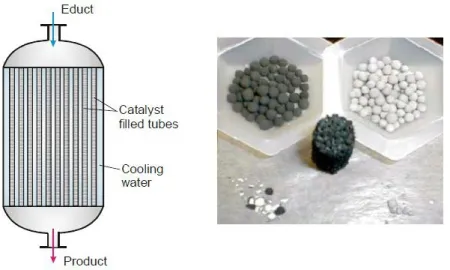
3.2 Reactor and catalyst used for the oxidization process. . . 36

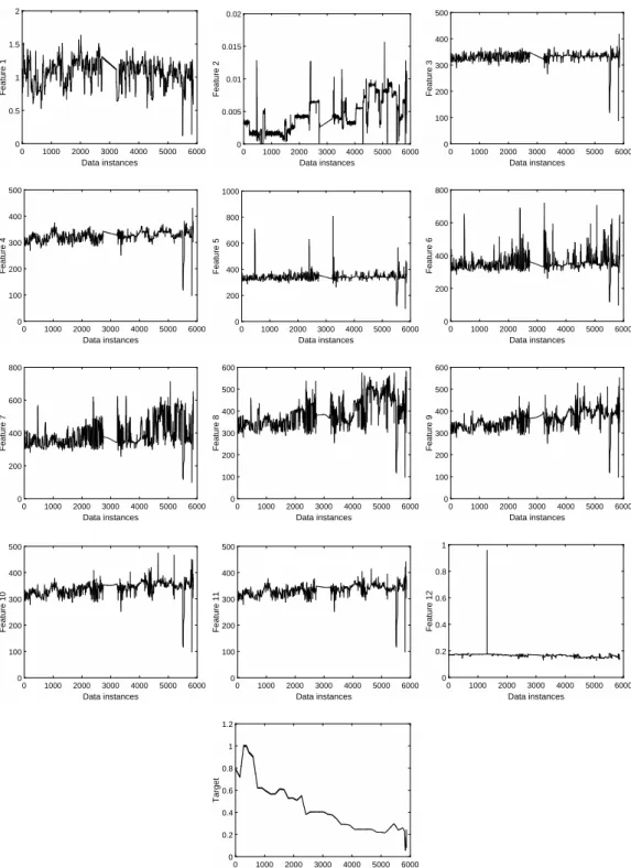
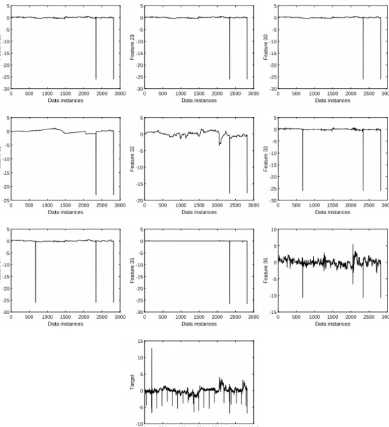
3.3 Catalyst dataset features and target value. . . 37

3.4 Oxidizer dataset features and target value. . . 40

3.5 Drier dataset features and target value. . . 42

3.6 Catalyst100 errors and symmetric Kullback-Leibler divergence values. . . 43

3.7 Oxidizer100 errors and symmetric Kullback-Leibler divergence values. . . 43

3.8 Drier100 errors and symmetric Kullback-Leibler divergence values. . . 44

3.9 Histograms of symmetric Kullback-Leibler values for all datasets. . . 45

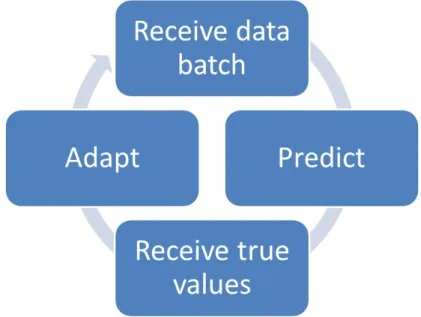
4.1 Assumed workflow of the prediction and adaptation on streaming data. . . 47

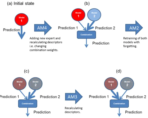
4.2 Adaptation with multiple adaptive mechanisms. . . 48

4.3 Block diagram of SABLE. . . 49

4.4 SABLE descriptor. . . 51

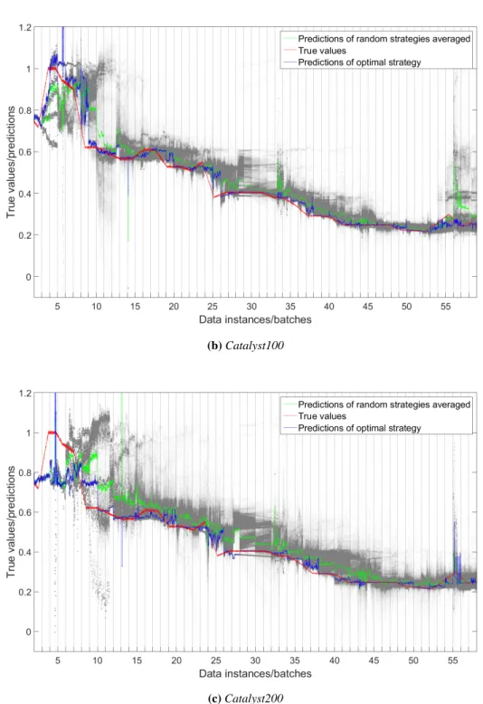
4.5 An example of a model adaptation sequence using SABLE adaptive mechanisms. 54 4.6 True/predicted values for Catalyst datasets. . . 57

4.7 True/predicted values for Oxidizer dataset. . . 60

4.8 Error values for Drier dataset. . . 63

5.1 Exhaustive 4-step ahead adaptive mechanism deployment on Catalyst100. . . 67

5.2 Relative adaptation histograms for Catalyst dataset. . . 71

5.3 Relative adaptation histograms for Oxidizer dataset. . . 72

5.4 Relative adaptation histograms for Drier dataset. . . 74

5.5 Scatter plot of adaptive vs non-adaptive errors for Catalyst100 dataset. . . 75

5.6 Scatter plot of adaptive vs non-adaptive errors for Oxidizer100 dataset. . . 75

5.7 Scatter plot of adaptive vs non-adaptive errors for Drier100 dataset. . . 76

5.8 Adaptive mechanisms generated byOptimalstrategy for the Catalyst dataset. . . 80

5.9 4 step ahead exhaustive adaptive mechanism deployment on all batches of Cata-lyst50 dataset. . . 80

5.10 NormalizedXVSelectresults’ comparison with different batch sizes. . . 81

5.11 Predictions on Catalyst50 dataset. . . 82

5.12 Adaptive mechanisms generated byOptimalstrategy for the Oxidizer dataset. . . 84

5.13 4 step ahead exhaustive adaptive mechanism deployment on all batches of Oxi-dizer50 dataset. . . 84

5.14 Predictions on Oxidizer50 dataset. . . 85

5.15 Adaptive mechanisms generated byOptimalstrategy for the Drier dataset. . . 87

5.16 4 step ahead exhaustive adaptive mechanism deployment on all batches of Drier50 dataset. . . 87

5.17 Drier50 dataset error values . . . 88

5.18 Pseudo-classifier MAE for Catalyst100 dataset. . . 89

5.19 Pseudo-classifier MAE for Oxidizer100 dataset. . . 90

5.20 Pseudo-classifier MAE for Drier100 dataset. . . 91

A.1 Using windows for expert adding condition and training data of a new expert. . . 106

A.2 Changes in experimental datasets. . . 108

A.3 Average accuracy values and ensemble sizes for selected methods. . . 112

A.4 Results grouped by the drift magnitude. . . 112

A.5 Results grouped by noise levels. . . 113

A.6 Results grouped byβvalue. . . 113

A.7 Results grouped by window size. . . 114

A.8 Power supply from main grid. . . 116

A.9 Results on Elec2 with different values ofβ. . . 116

A.10 Results on PowerItaly with different values ofβ. . . 116

2.1 Summary of ensemble adaptation methods. . . 25

3.1 Number of batches per each batch size for the used datasets. . . 36

4.1 SABLE parameters for different datasets. . . 55

4.2 Results of deploying random adaptive mechanism sequences on Catalyst dataset. 58 4.3 Results of deploying random adaptive mechanism sequences on Oxidizer dataset. 61 4.4 Results of deploying random adaptive mechanism sequences on Drier dataset. . . 61

5.1 Data generated using exhaustiver-step ahead adaptive mechanism deployment. . 69

5.2 Adaptive strategies. . . 78

5.3 Catalyst dataset results. . . 79

5.4 Oxidizer dataset results. . . 83

5.5 Drier dataset results. . . 86

5.6 Meta-features for adaptive mechanism prediction. . . 92

5.7 Adaptive mechanism classifier average accuracy values. . . 93

5.8 Results obtained using meta-classifier. . . 93

5.9 Confusion matrix of adaptive mechanism predictions for Catalyst50. . . 94

5.10 Confusion matrix of adaptive mechanism predictions for Catalyst100. . . 94

5.11 Confusion matrix of adaptive mechanism predictions for Catalyst200. . . 94

5.12 Confusion matrix of adaptive mechanism predictions for Oxidizer50. . . 94

5.13 Confusion matrix of adaptive mechanism predictions for Oxidizer100. . . 95

5.14 Confusion matrix of adaptive mechanism predictions for Oxidizer200. . . 95

5.15 Confusion matrix of adaptive mechanism predictions for Drier50. . . 95

5.16 Confusion matrix of adaptive mechanism predictions for Drier100. . . 95

5.17 MAE values over all batches after simple and cost sensitive meta-classification. . 97

A.1 Experiments with window based conditions to add an expert. . . 107

A.2 Experiments with the data basis for experts and their validation. . . 107

A.3 Starting weights and weight update factors,β, used in experiments. . . 108

A.4 Synthetic datasets used in experiments. . . 109

A.5 Top and bottom performing methods. . . 110

A.6 Results on 26 synthetic datasets, averaged. . . 111

A.7 Prequeuntial accuracy on Elec2 dataset. . . 115

A.8 Prequeuntial accuracy on PowerItaly dataset. . . 117

C.1 Adaptive mechanism classification cost matrix for Catalyst50. . . 120

C.2 Adaptive mechanism classification cost matrix for Catalyst100. . . 120

C.3 Adaptive mechanism classification cost matrix for Catalyst200. . . 120

C.4 Adaptive mechanism classification cost matrix for Oxidizer50. . . 121

C.5 Adaptive mechanism classification cost matrix for Oxidizer100. . . 121

C.6 Adaptive mechanism classification cost matrix for Oxidizer200. . . 121

C.7 Adaptive mechanism classification cost matrix for Drier50. . . 121

Symbol Description

y Target value

ψ(·) Function of the real process which generates the data x Input instance

ξ Noise

ˆ

y Predicted output

f(·) Prediction function/predictive model

Θf Set of parameters off

V Whole dataset,V =V₁∪ · · · ∪V_K Vk Data batch at timek,Vk={Xk,yk}

Xk Input data in batchVk

y_k Target data in batchV_k

N Total number of instances

N∗ Number of instances in a batch (assuming batches of a same size)

Nk Number of instances ink-th batch

P(·) Probability

E[·] Expected value

λ Forgetting (decay) factor

τ Time

l Moving window size

s(·) Expert / predictor

S Set of experts,S={s1,· · ·, sI}

w Weight of an expert

W Set of weights,W ={w1,· · ·, wI}

ν Weights update function

β Weights update factor

Error value,= ˆy−y

Errors on the whole dataset k Errors on batchVk

c Class label

C Set of class labels,C={c1,· · · , cJ}

Z Product of probabilities of all inputs for Naive Bayes classifier

ζ Threshold to add a new expert for (Kolter & Maloof, 2005)

β Threshold to remove an expert for Dynamic Weighted Majority algorithm

Ω Period (Dynamic Weighted Majority)

ωc sum of weighted predictions for a classc(Dynamic Weighted Majority)

φ Distribution

α Significance level

Background

Symbol Description X Input data

Y Output data ˜

Y Estimates ofY

N Number of data instances

M Number of input variables

K Number of output variables

L Number of latent variables T Score matrix

t Latent vector

D Corresponding loading matrix d Column vector ofD

U Score matrix u Latent vector

Q Corresponding loading matrix q Column vector ofQ

V Input data residuals F Output data residuals R Regression residuals B Regression weights matrix

b Column vector ofB

(·)> Transpose of a matrix, e.g. P>

Recursive Partial Least Squares (RPLS)

Symbol Description

m Feature number

Di,m Descriptor ofm-th feature ofi-th expert

D Descriptors matrix

Vtr _{Training data}

v(xn) Weight forn-th instance

Φ(µm_n,Σ) Two-dimensional Gaussian kernel function

µ= (xm_n, yn) Mean value of Gaussian kernel function

Σ Variance matrix of kernel function withσat the diagonal positions

σ Kernel width

wi Weight ofi-th expert’s prediction

p p-value of t-test between two experts’ prediction errors

P Matrix of pairwisep-values between prediction errors of all experts

D0 _{Old descriptors matrix before their recalculation}

D1 _{New descriptors matrix after their recalculation}

δ0 Weight of an old descriptor

δ1 Weight of a new descriptor

Symbol Description

f− A prioriprediction function (before the adaptation)

f+ A posterioriprediction function (after the adaptation)

g Adaptive Mechanism (AM)

G Set of AMs,G={g1,· · ·, gH} Θg Set of parameters ofg

ghk AM deployed on batchk

f_k+h Predictive model adapted usingghk,f

+h

k =f

−h

k+1

r Number of steps for exhaustive deployment/retrospective correction ˆ

Yk Predictions ofYkby different models in the AM exhaustive deployment tree

S Cross-validation training subset

S Cross-validation test subset

h i Error measure

h i× Cross-validated error measure

hopt_k Index of optimal AM for batchk

ˆ

hk Index of AM for batchkpredicted by meta-classifier

υ Meta-classifier function χ Meta-features vector

C Meta-classifier classification cost matrix

The work contained in this thesis is the result of my own investigations and has not been accepted nor concurrently submitted in candidature for any other award.

Introduction

1.1

Background and motivation

An essential element of human understanding of the complex systems and phenomena is creation of models. “Models are graphical, mathematical (symbolic), physical, or verbal representation or simplified version of a concept, phenomenon, relationship, structure, system, or an aspect of the real world.”1The degree of how well the model reflects its object is calledaccuracy. Models are usually constructed using observations of the object of modelling which may entail information about its inputs, structure, and outputs. Modelling serves to explain the objects and provide insights about their behaviour. Models have been very useful in areas such as physics, quantitative finance, marketing, industrial processes, social sciences, weather forecasting and others. With the rise of computing power and the ubiquitous recording of data, the usage of models, and particularly computational models, has been rapidly increasing.

Often, models describe entities which are inherently subject to changes. For instance, in in-dustrial process modelling, these changes may be caused by degradation of the equipment, in climate modelling by the climate change phenomenon, in financial modelling by sudden crises, in enterprise modelling by merger of the organisations. Afterthe changes, the accuracy of the model which was constructedbeforethe change and was based on the outdated assumptions, will often deteriorate. For these kind of changing environments, the need for model’s adaptation is paramount. Depending on the type of the model there are different ways to adapt it.

This thesis specifically focuses on predictive modelling in machine learning. Machine learning is the science of learning patterns from observed data, to make predictions on new, previously un-seen data. These patterns are often formulated as models, which are built by applying algorithms to the historical data. Models can be then used to calculate the desired predictions.

In some cases, these predictive models concern static datasets. However, quite often the pre-dictive models are being applied to the new data which keeps getting generated by the underlying processes. This type of data is called streaming data (Wang et al., 2003). In fact, with the current

1

http://www.businessdictionary.com/definition/model.html

advances in data storage, database and data transmission technologies, streaming data becomes increasingly relevant. This fact may pose additional challenges, one of them being the changes in the data generating process.

If the model remains unchanged for the whole duration of machine learning process, it is called a static machine learning model. However in situations when such models are used to de-scribe dynamic processes, their accuracy might degrade. Specifically, in machine learning, this effect may be caused by changes in data distribution ( ˇZliobait˙e, 2011), changes in features’ rele-vance (Fern & Givan, 2000), novel classes and features (Gabrys & Bargiela, 1999; Masud et al., 2013). For instance, in manufacturing settings, where the process is being observed by various sensors, gradual wearing of a sensor, its sudden failure, removal, replacement or addition of a new type of sensors can cause all of the above mentioned changes. Other examples of real world changes affecting relevant predictive models are special events, terrorist attacks or competitions which influence plane tickets demand (Riedel & Gabrys, 2007; Lemke et al., 2009, 2013), net-work intrusions which adapt to bypass the installed firewalls (Lee et al., 2000), seasonal changes influencing many areas such as electricity or gas consumption (Kolter & Maloof, 2007), change in lighting which can seriously affect image recognition in videos (Thrun et al., 2006). It has been shown that a changed environment, which is no longer being reflected by the model, contributes to the deterioration of model’s accuracy over time, (Schlimmer & Granger, 1986a; Gabrys & Bargiela, 1999; Street & Kim, 2001; Gabrys, 2004; Klinkenberg, 2004; Kolter & Maloof, 2007; Sahel et al., 2007; Mart´ın Salvador et al., 2016c).

In many cases it is possible to alleviate accuracy deterioration. Several options are available for this purpose. One of them is regular retraining, or in other words, creation of new models. This could be time consuming and in some cases impossible, for example when the required historical data is not available any more. Alternatively, one might employ various proposed online learning and adaptation approaches. Their purpose is keeping the existing model and making itself-adapt to the possible changes in environment.

Adaptive approaches range from high-level general adaptation concepts (Holland, 1992; Grisogono, 2006) to more practical adaptive machine learning algorithms (Littlestone et al., 1991; Carpenter et al., 1992; Jacobs, 1995; Kolter & Maloof, 2007; Bouchachia et al., 2007; Tsakonas & Gabrys, 2013; ˇZliobait˙e & Gabrys, 2014). They show better results while predicting on syn-thetic and real-world dynamic data than traditional non-adaptive models. It has been proposed that adaptive machine learning be applied to many different areas, such as chemical processing (Kadlec et al., 2011; Grbi´c et al., 2013), network intrusion detection (Lee et al., 2000; Haag et al., 2007), video image and concept recognition (Thrun et al., 2006; Yang et al., 2007) and others. Adaptive models can originate in different research fields: statistical and probabilistic approaches, machine learning, computational intelligence and different combinations thereof.

Typically adaptation operates by reducing the weight applied to the parts of the historical data that are less similar to the current data, which may be implemented in a variety of ways. In addition, recent adaptive methods use more than one Adaptation Mechanisms (AMs). Employing

multiple AMs is more versatile than using a single one and has been found to lead to superior prediction performance (Kadlec & Gabrys, 2011; Jin et al., 2015b). In practice, most research has used AMs deployed in a fixed manner with the choice of deployment order set at model design time. The common choice is to deploy all of the AMs at the same time, however this does not always deliver the best results with some AMs potentially cancelling the effect of others or changing the model more than required (Bakirov et al., 2017).

The possibility of having multiple adaptive mechanisms working together in one system pro-vides additional ways of handling the adaptation. However this also makes the control over it more complex. As will be seen from Chapter 4, the choice of adaptive mechanism needs to be carefully considered to achieve optimal results. Otherwise there is a risk of degrading predic-tive accuracy. To the best of author’s knowledge, no works explicitly research multiple adappredic-tive mechanisms related issues for streaming data prediction.

The main topic of this PhD project is therefore the investigation of predictive systems with multiple adaptive mechanisms in a streaming non-stationary data setting, with the aim to ulti-mately assist in improving adaptation capabilities of such systems, which would in turn result in higher accuracy rates.

1.2

Aims and objectives of the PhD project

While realizing the complexity of the described issues and challenges, this thesis tackles certain aspects of the usage of multiple adaptive mechanisms. The aims of the project are listed in the following sections.

1.2.1 Analysis and categorization of methods with multiple adaptive methods

Despite the large volume of research dealing with adaptive predictive modeling, there seems to be a lack of work focusing explicitly on adaptation; it seems to be considered to have a secondary role in regards to the whole predictive algorithm. Therefore, one of the goals of the thesis is to facilitate research into adaptive predictive modeling, while focusing on adaptation mechanisms. The following objectives are specified for this purpose:

• Conducting a large survey of research dealing with this topic,

• Identifying the most commonly used adaptive mechanisms, and

• Categorizing them in a meaningful way, where categories include adaptation mechanisms with similar characteristics.

Completing these objectives will create a framework for research into adaptive mechanisms, con-ducted further in this thesis and elsewhere.

1.2.2 Investigation of the necessity of adaptive mechanism selection

It is quite feasible that the selection of AMs to deploy is a big factor in the predictive performance of the model. However, explicit research to support this proposition has not hitherto been con-ducted. Therefore, one goal of the thesis is devising a study which tests this proposal. This study includes the following objectives:

• Development of an algorithm for experimentation purposes which uses multiple AMs from identified categories to deal with changes.

• Development of an experiment which will investigate the importance of AM selection.

• Performing the experiments on datasets with different adaptation needs and analysis of results.

1.2.3 Research into strategies of adaptive mechanisms’ deployment

It has been found that AM selection plays a crucial role in the predictive performance. There-fore a research into the ways and order of AM deployment will be conducted. The aim of this research is suggesting strategies for AM deployment (adaptive strategies) and identifying how these strategies affect the predictive performance. More concretely, it is aimed to achieve the following objectives:

• Implementing popular adaptive strategies using the predictive algorithm from the previous section.

• Suggesting adaptive strategies which can provide better results than the common ones.

• Analysing the results, identifying the circumstances where different adaptive strategies work well and the reasons behind it.

1.3

Original contributions

‘ The main scientific contributions of this thesis are:

• Investigation of the importance of AM order selection (adaptive strategies). Using an empirical experiment on the real process industry data provided by project partner Evonik Industries AG, it was established that the selection of AM order is a significant factor for the predictive accuracy of the algorithm.

• Identification and performance analysis of different fixed and flexible AM strategies, suggestion of cross-validation based AM strategies and retrospective model correction technique. The performance of common fixed adaptive strategies and suggested flexible strategies on real datasets were compared and it has been found that flexible strategies suggested in this thesis outperform other strategies most of the time.

• Development of Simple Adaptive Batch Learning Ensemble (SABLE) online learning framework.An adaptive framework in plug-and-play fashion, where a number of AMs are deployable in various manners has been developed for the experimentation purposes.

• Categorisation and formalisation of adaptive mechanisms. A comprehensive survey of adaptive predictive algorithms has been conducted. The results of the survey were a base for the categorisation of commonly used adaptive mechanisms. A formal notation of adaptation process has been also introduced.

• Research into the criteria and training data of added global experts in streaming clas-sification problems.The effects of different sizes of training data for newly added experts, different conditions for their addition have been empirically analysed.

1.4

List of resulting publications

The research leading to these contributions has resulted in the following publications:

• Bakirov, R; Gabrys, B. Investigation of Expert Addition Criteria for Dynamically Changing Online Ensemble Classifiers with Multiple Adaptive Mechanisms In: Artificial Intelligence Applications and Innovations, 646–656, 30 September–2 October 2013, Paphos, Cyprus.

• Bakirov, R.; Gabrys, B. and Fay, D. On Sequences of Different Adaptive Mechanisms in Non-Stationary Regression Problems. In: 2015 International Joint Conference on Neural Networks 12 July–17 July 2015, Killarney, Ireland

• Bakirov, R.; Gabrys, B. and Fay, D. Augmenting Adaptation with Retrospective Model Cor-rection for Non-Stationary Regression Problems. In: 2016 International Joint Conference on Neural Networks 24–29 July 2016 Vancouver, Canada.

• Bakirov, R.; Gabrys, B. and Fay, D., Multiple adaptive mechanisms for data-driven soft sensors Computers and Chemical Engineering, vol. 96, pp. 42–54, 2017.

1.5

Organisation of the thesis

Following this introductory chapter, the thesis is organised as follows. Chapter 2 presents back-ground information about predictive modeling on streaming data and gives details of existing adaptive mechanisms. AMs’ hierarchical categorization is proposed, and several types of base learners used in predictive methods with multiple adaptive mechanisms are introduced. The de-tails of these predictive methods are given as well. Chapter 3 gives short information about the process industry, where the considered data sets for experiments are originating from, further in-troduces these datasets and analyses their characteristics in regards to exhibited changes. Chapter 4 looks into whether deployment of different AM sequences affects the accuracy of a predictive model. Here the predictive model with multiple AMs, which is used as a vehicle for experi-mentation, is introduced in detail. Chapter 5 analyses the effects of different AMs, identifies and conducts experiments with many traditional adaptive strategies as well as with the proposed novel ones. The results are compared and it is analysed which strategies provide better predictive accu-racy and what are possible reasons for this. Chapter 6 gives an overview of the findings, provides concluding remarks and possible future research directions. An investigation into expert addition

Learning and adaptation on streaming

data

2.1

Introduction

With the rise of streaming data analytics, it is becoming increasingly more important to be able to incorporate new data in predictive models as well as to be able to react to changes in the data. A variety of adaptive learning methods on streaming data (e.g. (Schlimmer & Granger, 1986a; Kolter & Maloof, 2007; Kadlec & Gabrys, 2011; Elwell & Polikar, 2011; Lemke et al., 2013; ˇZliobait˙e & Gabrys, 2014; Gomes Soares & Ara´ujo, 2015b)) have been developed for these purposes. In recent times this type of methods often features multiple adaptive mechanisms, (e.g. (Castillo & Gama, 2006; Kolter & Maloof, 2007; Kadlec & Gabrys, 2011; Minku & Yao, 2012; ˇZliobait˙e et al., 2012; Gomes Soares & Ara´ujo, 2015b; Bakirov et al., 2017)) increasing the number of ways they can deal with these issues, and potentially providing better predictive performance.

This chapter introduces the key concepts in adaptive learning, which is the area of Machine Learning dealing with non-stationary data. The chapter starts by presenting general techniques of learning and adaptation on streaming data in Section 2.2. It lists the types of learning/adaptation in this setting, as well as the possible reasons why the adaptation might be needed (Section 2.3.1). Then in Section 2.4 it proceeds to explore adaptation in machine learning in a greater detail. The different types of adaptation mechanisms, starting with the ones which adapt the coverage of available training data and continuing with the adaptation of models’ parameters and structure, are identified and categorised. In Section 2.5 a more detailed analysis of ensemble methods is given, since these are the methods which are the most relevant to the research produced in this thesis. Finally, the methods which employ multiple adaptive mechanisms are discussed in Section 2.6.

2.2

Learning on streaming data

In many applications, existing predictive models are being constantly applied to new data and after a certain time some or all true target values become available. This is the case for instance with credit scoring where the goodness of credit is revealed only after some time (Dal Pozzolo et al., 2015), process industry where lab measurements can be much slower than the process (Kadlec & Gabrys, 2011), stock market predictions (Hazan & Seshadhri, 2009) and other areas. The natural question is, how is it possible to use this new information to improve the accuracy of the models. To give a mathematical formulation, it is assumed that the data is generated by an unknown dynamic process which can be formulated as:

y=ψ(x) +ξ, (2.1)

whereψis an unknown function,ξa noise term,x∈_RM _{is an input data instance, andyis the}

observed output. Then the predictive model as a function:

ˆ

y=f0(x,Θf|V0), (2.2)

is considered, where yˆis the prediction, f0 is an approximation (i.e. the model) ofψ(x), and

Θf is the associated parameter set. It is assumed that the f0 was built using some training set V0 = {X0,y0}. At some point, new data from the process, V1 = {X1,y1} is obtained.1

The goal of learning in this case is to use new data,V₁, to improve the predictive model,f0. As

having a larger training dataset typically increases predictive accuracy, learning new data is useful especially in the cases when the initial dataset might have been insufficient to achieve the desired performance.

Methods to learn new data operate in several ways. Most straightforwardly, they combine both historical and new data to generate a new dataset, which will be used to train a new model, thereby updating the old model with new information (Figure 2.1(a)). Essentially a new predictive model

f1(x,Θf|V0∪V1) (2.3)

is created. This approach is possible for all types of learning algorithms (e.g. decision trees (Quinlan, 1993) (Breiman et al., 1984), model trees (Quinlan, 1992), SVM (Vapnik, 1995)) as long as the required data is available. However this is often not possible or not the ideal solution; historical data might not be available2 any more or building a model from scratch might be too time or resource consuming. Methods called online learners, such as Recursive Least Squares (Plackett, 1950) or naive Bayes (Hastie et al., 2009) which instead of explicitly combining the data to form a new dataset, achieve the same effect without requiring access to old data are preferred for

1_{For brevity purposes, Equation 2.2 will be shortened asyˆ=f}

0(x)in this thesis.

2

Even when all historical data is available, using it may also not be a good/possible choice when it is not relevant to or compatible with new data. This requires adaptation, discussed in Section 2.3

such cases. These algorithms store only the model characteristics (e.g. counts, linear coefficients, etc.) and update them when new data arrives (Figure 2.1(b)). This can be formulated as

f1(x,Θf|f0,V1). (2.4)

Online variations for many popular off-line machine learning algorithms specified above have been also developed (Cauwenberghs & Poggio, 2001; Hulten et al., 2001; Kivinen et al., 2004; Potts & Sammut, 2005).

Figure 2.1:Learning new data: a) using historical data b) online learning.

Methods for learning on streaming data fall into two types; incremental and batch learning. Incremental learning is learning from a single new data instance.3 While being able to learn one-by-one is certainly a powerful asset, in many practical situations the data becomes available in small batches over a period of time, as noted in (Polikar et al., 2001). For these cases, incre-mental learning is often redundant and potentially inefficient. The second group of models, batch learners, operate on whole batches of data simultaneously, and are better suited to this scenario. Naturally batch learners may also operate in the scenarios when data instances are arriving one-by-one by waiting until the required amount of new data is available, which however slows down the reaction to the changes. Batch learning allows the creation of new experts based on a con-siderable amount of data increasing the stability of predictions (Elwell & Polikar, 2011) and the measurement of metrics on a batch to potentially use them as meta-features (Alippi et al., 2012). Methods such as Naive Bayes and online versions of popular algorithms, for instance Recursive Least Squares Estimator (Plackett, 1950), Recursive Partial Least Squares (Joe Qin, 1998) and others are capable of both incremental and batch learning.

Streaming data learning algorithms can further be differentiated by their ability to use old data for learning, number of passes performed on the data, the ability to learn previously unseen classes

3

and the ability to retain prior learned knowledge. This chapter reviews works from different research directions, where the only requirement is the learning of information from new data.

2.3

Adaptation for predictive models on streaming data

In a static machine learning setting the parameters of the model are trained using a historical data set and then fixed with no modifications as the process continues regardless of the observations. This approach assumes that there are no significant changes in the process throughout the duration of the model’s usage, or that those changes would not significantly degrade the performance of the model. However, this is not always the case. As noted in Chapter 1, machine learning is often applied to dynamic non-stationary environments where changes of various types are common. These changes often result in reduced predictive accuracy of the models or sometimes and more dramatically could even render the current model technically inapplicable to the new environment (this is discussed in more detail in next section).

Dealing with changes requires using the current data either for building a new model (and discarding the existing one) or adapting the existing one. Adapting a model involves reducing the effect of old and irrelevant data, and is often the preferred choice, especially when the current data may not be large enough to build a meaningful model or when the old knowledge needs to be preserved. It is possible to see that the concept of adaptation is closely related to the concept of learning new data, because it is precisely the new data that prompts adaptation. Learning new data can be to some extent considered to adapt a model, in a sense that with the increase in the amount of new data, the effect of old data is gradually reduced. However, simply learning new data after a change improves model’s accuracy much slower than its explicit adaptation (Kuncheva, 2004a; Kolter & Maloof, 2007). It should also be noted that depending on the implementation, it is not always possible to simply learn data after certain types of changes in the data, e.g. after the change in input features.

2.3.1 Reasons for adaptation

The reason for the adaptation of predictive models is that, given the available data, a new model which performs significantly better than the existing one can be trained. This happens if:

• The model is inapplicable to the new data. This situation often occurs after the changes in the definition of data, for instance when number of features or their domains change. For example when a platform where the videos are rated using “thumbs up/down” ranking is switched to 5 stars ranking, the models trained to predict videos’ ranking using the old system, would not be suitable for the new data, resulting in useless predictions. Depending on the algorithm, these type of changes might render the outcome meaningless, or prevent the model from making predictions whatsoever. It should be noted that certain changes of this kind may be addressed using pre- or post-processing techniques, for example treating

removed features as missing data, however these type of solutions may not be adequate for the long term.

• Alterations to the model would better explain the observations. Other types of changes can lead to situations where the model delivers meaningful predictions, however its accuracy could be further improved. This is often manifested by the deterioration of the predictive accuracy over time. This can be more formally depicted as follows:

E[f(xτ0)]< E[f(xτ1)] (2.5)

whereE[f(x)]is the expected error of the predictive function,xτ0,xτ1 are the input data

instances at timesτ0, τ1, τ1 > τ0. In other words, the increase of the expected error over

time means that the deterioration of the accuracy takes place. The types of changes in the real world causing this can be varied; these could be wear of sensors for process indus-try models, market perturbations in financial modelling, change of light settings in image recognition etc. In general, this is often a result of a change in input-output conditional probability of the data generation process, which is also known as concept drift.

The work in this thesis will be mainly focused on the second type of changes, however some of the discussed techniques are applicable to the first type as well.

2.3.1.1 Concept drift

One of the most researched and well defined reasons for the adaptive models is the problem of concept drift, as introduced in (Schlimmer & Granger, 1986b) or (Widmer & Kubat, 1996). Using the probabilistic formulation from (Gao et al., 2007), joint input-output probability is given by P(x, y) = P(y|x)· P(x). Concept drift occurs when either the independent probability distributionP(x)or conditional probability distributionP(y|x)changes with time4. The former is often called virtual and the latter real concept drift. Many authors, e.g. (Tsymbal et al., 2008) or ( ˇZliobait˙e, 2009) note that for practical purposes, these two types can be considered the same in that they both require changes in models. In (Elwell & Polikar, 2011) it is stated that, virtual drift requires supplemental learning or refining of the model and real drift requires replacement learning or forgetting. In the terms of change speed and behaviour the following categories of drift are identified in the literature (Gama et al., 2014):

• Sudden drift. This is sudden change of concept at a certain timeτ.

• Gradual drift. Occurs when one concept gradually replaces another over certain time period

τ2−τ1.

• Incremental drift. This is a slow change involving the passage through intermediate con-cepts between the concon-cepts before the drift has started and the final concept after the drift is finished.

4

Figure 2.2:Concept drift types (Gama et al., 2014).

• Reoccurring concepts. Concepts are replaced by the new ones, only to reappear at the later stage. This is typical for cyclical and seasonal processes.

Figure 2.2 visualizes types of drift. Although the notion of concept drift appears more often in classification scenario, there are works which use this concept in regression setting as well (Ikonomovska et al., 2010; Gomes Soares & Ara´ujo, 2015a,b). For a recent survey on concept drift, reader is referred to (Gama et al., 2014).

2.3.2 Adaptation for predictive modelling

As mentioned in the previous section, this thesis concentrates mainly on the accuracy of the pre-dictive models. Therefore a following definition can be used:Definition:Adaptation is an update of combination of the model’straining data coverage,structure, andparametersto optimize pre-dictive accuracy in order to respond to the changes in the data.

These changes may include the ones listed above. Adaptation also learns new data, however the difference between simply learning new data and adaptation based on new data is that the goal of simple learning isrefiningthe model, and the goal of adaptation ischangingit. The methods for both types of learning can be similar. However, due to the temporal nature of adaptation, many adaptive learning methods assume that the data before the change is less relevant for the new model than the data after change. As a result of this assumption, these methods tend to give more weight to the newer data instances than to the older ones while constructing the models.

An important aspect of adaptive models is when the adaptation process is triggered. Some models use change detection routines for example described in Basseville & Nikiforov (1993); Gama et al. (2004); Baena-Garc´ıa et al. (2006) to attempt to detect when the model needs adap-tation. Stationarity tests such as tests pioneering Priestley-Subba-Rao test (Priestley & Subba Rao, 1969) or more recent approaches described in (von Sachs & Neumann, 2000; Nason, 2013; Balaguer-Ballester et al., 2014) may be also applied for this purpose. If the change is correctly detected, these approaches avoid needless adaptation, therefore allowing for more robust models. However, as change detection is no trivial task, other approaches prefer to adapt the models in regular time intervals without additional triggers (Stanley, 2002; Elwell & Polikar, 2011; Scholz & Klinkenberg, 2007; Jacobs et al., 2010). This ensures a guaranteed response to the changes, however risks the overreaction to noise on one hand, and delayed adaptation on another hand, subject to the parameter choice. In classification scenario, triggering adaptation after every mis-classification is also practised (Kolter & Maloof, 2005, 2007).

Figure 2.3:General adaptations scheme.

There are various adaptive predictive algorithms in the machine learning literature. They use adaptive mechanisms which can be categorized into several types. The next sections present a detailed overview of these adaptive mechanisms.

2.4

Overview of adaptive mechanism types

In this section a hierarchical structure of adaptive mechanisms types is presented. More con-cretely, on the lowest tier of the hierarchy the object of adaptation is the underlying training set of the model, and on the higher tiers its parameters and structure. This hierarchy is depicted on Figure 2.3. Here, the hierarchy is meant in a sense that the application of an adaptive mechanism of the higher level, requires the application of the adaptive mechanism of lower level. It should be noted that, depending on the adaptation settings, the effects of adaptive mechanisms on each level can be differently strong. Evolutionary adaptation approaches which construct a special niche are also discussed in Section 2.4.4.

2.4.1 Adapting training data coverage

The basic adaptive mechanism is updating the coverage of models’ training data set to give more weight to recent data. The most commonly used techniques for this purpose are moving window and decay factors approaches as discussed in Sections 2.4.1.1 and 2.4.1.2. For some methods which do not build an explicit general model for the prediction of new data instances, also known as lazy learning methods, such as k-nearest neighbours (Hastie et al., 2009), just an updated dataset will instantly change the output of the model. For the methods which do construct a gen-eral prediction model, also calledeagerlearning methods (e.g. linear regression, SVM, decision trees), new data prompts the update of the model’s parameters or structure, which is discussed in

the sections below.

Deciding which subset of data to use as training set is one of the paramount questions that needs to be answered while developing an adaptive predictive algorithm. Generally it is assumed that, in the case of no changes in the process, the more data is included in the training set, the lower the variance of the parameter estimates will be, thus increasing the predictive accuracy. It has been shown that the size of the training data sufficient to achieve the desired accuracy is determined by the VC dimension5of the algorithm (Blumer et al., 1989; Anthony & Biggs, 1997; Vidyasagar, 1997). More practically, it is determined by the total number of free parameters and permitted error (Haykin, 2009).

In non-stationary data setting, it becomes important to not only select a training set of suf-ficient size but also one which is relevant to the current data. The parameters of the adaptive approaches determine the scale of reducing the influence of the old data. Less influence leads to faster adaptation, however, it also increases the leverage of noise or structural changes in the recent past. Conversely, increasing the influence of older data reduces the rate of adaptation, but at the same time creates more robust models. This is called thestability-plasticitydilemma (Car-penter & Grossberg, 1987) in adaptive learning. Sometimes data which is considered irrelevant is simply discarded. This is called “forgetting” (Kuh & Petsche, 1990) or “catastrophic forgetting” (Polikar et al., 2001) and can be detrimental if the discarded data becomes relevant in the future. Popular approaches to choose the training data for the model are moving window and decay fac-tors. It should be noted that not all of the approaches require to explicitly store the old data as online learning methods which are often used for adaptive models implicitly update their training sets when the new data becomes available.

2.4.1.1 Moving window approaches

The moving window approaches limit the training data for predictive model at timeτ to the most recently seenlinstances asV ={(xτ−l, yτ−l),· · · ,(xτ, yτ)}wherelis the size of the window.

The advantages of this approach are its simplicity and effectiveness in many cases (Widmer & Kubat, 1996). The window size is the only parameter, and is critical in controlling how fast the adaptation is performed. The speed of adaptation is inversely proportional to the size of the win-dow. However insufficient training data might result in more inaccurate models, and overreacting to noise. While lis usually fixed, works such as (Widmer & Kubat, 1996; Klinkenberg, 2004) propose heuristics for an adaptive window size which proves to be more beneficial, particularly when dealing with random changes. (Widmer & Kubat, 1996) propose to increase the window when the input data is stable and decrease it when concept drift occurs. (Klinkenberg, 2004) sug-gests testing several sizes of windows on the latest data batch and choosing the one that performs the best. In many scenarios, for example if a single model is created from the sliding window, it is beneficial to set window size so that its contents exhibit stationary behaviour. Stationarity tests

mentioned in Section 2.3.2, (Priestley & Subba Rao, 1969; von Sachs & Neumann, 2000; Nason, 2013) may be used for this purpose. The moving window approaches are usually based on the time of data instances’ arrival, however the similarity of training data to the current data can also be considered for this purpose.

2.4.1.2 Decay

One could view a window approach as weighting vector of ones applied to the most relevant data, and zeros to the rest of data. In a more general case, a continuous decreasing weight could be applied. The simplest approach is to use a single decay factor λ <1. The repeated use of this decay factor leads to the exponential reduction of data’s weight. Decay can be based not only on time of instances’ arrival (Joe Qin, 1998; Klinkenberg & Joachims, 2000), but also on similarity to the current data (Tsymbal et al., 2008), combination thereof ( ˇZliobait˙e, 2011), density of the input data region (Salganicoff, 1993b) or consistency with new concepts (Salganicoff, 1993a). Non-exponential decay approaches also exist, for example autoregressive model (Mills, 1991).

2.4.2 Adaptation of predictive models’ structure

Structure of predictive model is the set of its components and the way these components are con-nected to each other. Some model types actually define a family of models with different possible structures. For example, a 2-layer feed-forward neural network may have different number of nodes. Adding or removing a node does not change the nature of the model in this case. Struc-ture of the predictive model could be for example, hierarchical (for example decision trees) or graph-like (Bayesian or neural networks). Here, the structure is not necessarily limited to the topological context – number of rules in rule based systems or number of experts in an ensem-ble could be considered part of the model’s structure. Updates in the models’ structure are also used for the adaptation purposes, often changing the model more radically than update of the parameters would be able to accomplish. Relevant examples are listed below:

• Decision trees.There is a considerable amount of research dedicated to decision trees with updatable structure. For instance, Very Fast Decision Trees (VFDT) for classification by (Domingos & Hulten, 2000) incrementally grows the tree with the arrival of new observa-tions and its extension Concept-adapting Very Fast Decision Tree (CVFDT) (Hulten et al., 2001) uses a sliding window approach to deal with concept drift. The regression-capable online decision tree introduced in (Basak, 2006) is also capable of altering the tree structure, albeit with a fixed tree depth.

• Model trees. Structural updates are also applied for model trees. For instance, (Potts & Sammut, 2005) propose an incremental algorithm with the strategy of splitting the node if it is statistically unlikely that the examples in it are generated by a linear model. A method proposed in (Ikonomovska et al., 2010) can replace a subtree with a leaf or grow an alternative subtree if a change is detected.

• Neural networks. Although most of the existing neural network architectures use a fixed structure once trained, some developments indirectly include the ability of changing net-works’ structure after retraining by using variable nodedropoutprobabilities (Ba & Frey, 2013). Another neural-network based approach used for online learning, and capable of adapting its structure, is the ARTMAP family of methods (Carpenter et al., 1991; Vakil-Baghmisheh & Paveˇsi´c, 2003). It adds nodes to accommodate for new classes which are encountered during the prediction process.

• Bayesian networks. The Bayesian network as proposed in (Pearl, 1988) is an approach which aims to capture causal relationships between features and model them as a direct acyclic graph using Bayes’s theorem. Updating Bayesian networks’ structure is described in research such as (Friedman & Goldszmidt, 1997; Lam, 1998; Alcob´e, 2004). (Castillo & Gama, 2006) propose a multi level adaptation scheme for a Bayesian network, which involves both changing its parameters and structure.

• Ensemble methods.Adding or removing experts (e.g. in (Stanley, 2002; Kolter & Maloof, 2007; Hazan & Seshadhri, 2009; Gomes Soares & Ara´ujo, 2015b)) is an important adapta-tion mechanism for adaptive ensemble methods, and can be considered a structural change. This is discussed in greater detail in the Section 2.5.3.

.

2.4.3 Adaptation of predictive models’ parameters

Most of the predictive models’ predictions are dependant on a number of parameters (see Equa-tion 2.2), which may be adjusted to adapt the model. Training the model in this case comes down to estimating these parameters and adapting it involves updating the parameters as new data instances are available. Many popular algorithms have online versions to be able to update their parameters faster than retraining them from scratch and to not require the historical data. Following examples can be considered:

• Linear regression. For linear regression the set of parameters are the linear coefficients, which can be estimated using different methods, such as Ordinary Least Squares Estima-tion. There are many types of linear models where the coefficients are allowed to change with time. An example of these is adaptive version of Least Squares Estimation described in (Jang et al., 1997). It recursively updates the parameters, optionally employing the de-caying of the weights of old observations.

• Naive Bayes classifier.The parameters of Naive Bayes classifier (described in more details in Section 2.5.1.1) are the prior probabilities of classes and conditional probabilities of features given classes. These are calculated during the training of the model and could be incrementally updated during the prediction process by saving sums and counts of features, and number of observations.

can be updated with each learned instance using for example back-propagation algorithm (Werbos, 1974). As back-propagation does not provide explicit control over the adapta-tion, neural networks which use it or similar training methods can be prone to catastrophic forgetting (Kasabov, 2001). Several approaches address this problem. For instance, experi-ence replay(Lin, 1992) stores a set of old instances in memory and uses them along with the new ones to train the network. This approach has been successfully used recently in Deep Q-Network (DQN) algorithm (Mnih et al., 2015). Another solution of forgetting problem, which has become very popular in recent years is Long Short-term Memory (LSTM) ar-chitecture introduced in (Hochreiter & Schmidhuber, 1997) and recently analysed in (Greff et al., 2016). LSTM deals with this issue using special blocks which assist the network to control the forgetting.

• Ensemble methods.Expert weights are an important parameter of the ensemble methods. They are often recalculated using the new data or updated in various ways (Littlestone & Warmuth, 1994; Kolter & Maloof, 2007; Elwell & Polikar, 2011; Kadlec & Gabrys, 2011; Bakirov et al., 2017). This is discussed in more detail in the Section 2.5.2.

2.4.4 Evolutionary approaches

A family of methods collectively called evolutionary approaches practice adaptation which is loosely based on the theory of evolution. These approaches involve having a population of so-lutions, adding new members using certain operations like mutation and crossover, and selecting the “fittest” members from the population based on some fitness criteria. One group of evolution-ary methods which are able to operate on streaming data are Learning Classifier Systems (LCS), introduced in (Holland, 1976). LCS work with a pool of rules where new rules are created if no existing rules are relevant for new examples, and also by constant application of genetic operators and selection of the best rules using a fitness function. The approach combines both exploration by selecting a random passing rule to determine the action (or label) and exploitation by select-ing an action which has maximum combined fitness among all the passselect-ing rules. One example of LCS for classification is sUpervised Classifier System (UCS) (Bernad´o-Mansilla & Garrell-Guiu, 2003). Further example are evolutionary mechanisms and algorithms applied in the context of multi-component multi-level predictive systems (Gabrys & Ruta, 2006; Tsakonas & Gabrys, 2012, 2013; Lemke et al., 2013).

Another interesting area of population based techniques are Artificial Immune Systems (AIS) (Castro & Zuben, 1999) which simulate the human immune system. Simplistically described, AIS create and maintain a pool of antibodies for recognising the threats to the organism via genetic operations and try to increase diversity of this pool for better recognition abilities. Antibodies gradually age and are replaced with new ones. Ageing speed is inversely proportional to their recognition rates, which means that antibodies that are less effective are replaced faster and the ones that are more effective are replaced slower. Some characteristics of AIS, such as adaptation,

forgetting and ability to deal with new threats make it potentially very useful for non-stationary streaming data. For example (Abi-Haidar & Rocha, 2008) apply AIS methods to spam detection and (Haag et al., 2007) use them for network intrusion detection. A survey of AIS research can be found in (Dasgupta et al., 2011).

2.5

Ensemble methods

A popular approach in machine learning is combining multiple models (which in this scenario are often called “predictors”, “learners” or “experts”6) for predictions (Ruta & Gabrys, 2000). Ensemble methods were originally developed in 1960-s for static data (Bates & Granger, 1969), but have gained widespread use for streaming and non-stationary data as well. In the static setting the ensembles are widely used for “boosting”, which aims to increase the prediction accuracy for parts of the input space where accuracy is low (Freund & Schapire, 1995), or “bagging”, which aims to increase the generalising ability of a predictive model (Breiman, 1996). (Dietterich, 2000) presents three reasons why ensembles of experts often perform better than single learners in stationary settings:

• Statistical: many models can perform quite similar on training data but differently on the test data. To eliminate the risk of choosing a poor model, a safer choice would be using them all in the ensemble and average their predictions.

• Computational: many experts reduce the risk of getting stuck in local optima during the learning process.

• Representational: in many situations the concept might be represented better by the weighted sum of multiple learners rather than a single learner.

The drawback of combining multiple learners is that the resulting model will have higher com-plexity than using a single learner (Kuncheva, 2004b). Moreover, it has been also shown that it can be very beneficial to organise predictions in multiple layers (Ruta & Gabrys, 2002, 2005) (simi-larly to the recently popularised deep neural network structures) leading to even further increase in the of the complexity of the resulting system together with a great potential performance gain. This has been illustrated in many sucessful experimental studies carried out in author’s group (Ruta & Gabrys, 2005, 2007; Riedel & Gabrys, 2007; Lemke et al., 2009; Budka et al., 2010; Ruta et al., 2011; Tsakonas & Gabrys, 2012, 2013; Lemke et al., 2013; Mart´ın Salvador et al., 2016b).

In a streaming data setting, experts are used to improve the generalisation properties of the model and to serve as a representation for historical data. In addition, in a non-stationary setting, some models attempt to align experts with concepts as they arise (Kadlec & Gabrys, 2011; Shao & Tian, 2015; Jin et al., 2015a).7 Many studies (e.g. (Kolter & Maloof, 2007; Elwell & Polikar, 2011; Kadlec & Gabrys, 2011)) have found that adapting ensemble combination weights, for

6

These terms are used interchangeably throughout this thesis.

7

instance based on experts’ prediction accuracy, is an effective method of dealing with changes in the data. Often the combination weights of ensemble members are updated at a rate inversely proportional to their prediction errors. More concretely,w1 =ν(1, w0), wherew1 is the weight

after the update, andν(·)is the update function, its inputs being error1and optionally previous

weightw0. For instance, the update function can be realised as ν(1, w0) = w0e− (Herbster

& Warmuth, 1998). When the input w0 is absent, the weight update function takes the form of

w1 =ν(1)and essentially becomes weights recalculation, used for instance in (Elwell & Polikar,

2011). Experts may be separately updated (Kolter & Maloof, 2007) or adapted using moving windows or forgetting factors (Kadlec & Gabrys, 2011; Bakirov et al., 2015). Creation of new experts from newly arrived observations is another useful strategy to learn new information which has been found to provide good results (Klinkenberg, 2004; Wang et al., 2006; Kolter & Maloof, 2007; Elwell & Polikar, 2011). An alternative to combination isgating, where a prediction of a single expert, which is considered the most relevant to the current state of the system, is selected as a final prediction of the ensemble.

Adaptive ensemble methods for learning on streaming data often feature all of the levels of AM hierarchy introduced in Section 2.4. Adapting individual expert may be realised via the training data coverage adaptation and the parameter adaptation levels. Adapting the combination weights may be considered a form of parameter adaptation and adding/removing experts an adaptation of model’s structure. In Sections 2.5.1, 2.5.2 and 2.5.3 a short overview of the most prominent adaptation methods and techniques belonging to each of these levels is presented.

2.5.1 Base learners and their adaptation

There are many choices for the type of models that can be used in an ensemble as the base learners, in fact any predictive model, including other ensembles, can be used for this purpose. For instance, machine learning methods such as linear regression (Kadlec & Gabrys, 2011; Gomes Soares & Ara´ujo, 2015b), naive Bayes (Bakirov & Gabrys, 2013), SVM (Scholz & Klinkenberg, 2007), decision trees (Street & Kim, 2001; Stanley, 2002; Bifet et al., 2009), neural networks (Polikar et al., 2001; Lan et al., 2009; Gomes Soares & Ara´ujo, 2015a), k-nearest neighbours (Masud et al., 2013) have been used as base learners. Base learners may be updated by explicitly or implicitly increasing their training data and may be adapted using adaptation mechanisms such as moving windows or decay factors (Sections 2.4.1.1 and 2.4.1.2). Examples of algorithms which employ learnable/updatable base learners are (Stanley, 2003; Kolter & Maloof, 2007; Bifet & Gavald`a, 2007; Kadlec & Gabrys, 2011; Grbi´c et al., 2013; Gomes Soares & Ara´ujo, 2015a,b; Shao & Tian, 2015; Jin et al., 2015b; Bakirov et al., 2017). However, it is not always the case that experts are adapted, as the adaptation can be performed purely at the combination level and/or via adding/removing experts. This is characteristic only to batch learning algorithms (e.g. (Scholz & Klinkenberg, 2007; Elwell & Polikar, 2011)).

(RPLS) which were used as base learners for experiments in this thesis.

2.5.1.1 Bayesian learning and Naive Bayes classifier

Bayesian learning is an inherently probabilistic approach for building predictive models in which unknown quantities are given a distribution based on observations. The distributions are updated and predictions are formed from the posterior. The core of Bayesian learning is Bayes’ theorem

P(A|B) = P(B_P|A_(B)P₎(A) which relates the of conditional probability ofP(A|B)(event Agiven

B) to the P(B|A) (likelihood of B given A; typically the observation given the model) and independenta prioriprobabilities of two eventsP(A)andP(B). In the classification setting this equation can be written as:

P(c|x) = P(x|c)P(c)

P(x) , (2.6)

wherecis a class label. The popular Bayesian learning method, Naive Bayes classifier, assumes the conditional independence of features from each other. Then, the classification problem comes down to estimating the probability of each class and determining the class with the highest prob-ability value, as:

P(c|x) = 1

ZP(c)Π

M

m=1P(xi|c) (2.7)

HereZ is a product of probabilities of all inputsP(x1),P(x2), ...,P(xM)which is constant for

all class labels. Returning to the described hierarchy, independent probabilities of classes/features and conditional probabilities P(xm|c), m ∈ 1· · ·M may be considered as the parameters of

Naive Bayes classifier. It is possible to incrementally update these values when new instances are observed. Despite the strong assumption of feature independence, the Naive Bayes classi-fier is widely used in practice, because of its usually satisfactory prediction accuracy, ease of implementation and inherent capability of online learning.

2.5.1.2 Recursive Partial Least Squares

Recursive Partial Least Squares is an extension of Partial Least Squares (Wold, 1966), both being popular in chemical process modelling. PLS projects the scaled and mean centered multidimen-sional input data X ∈ _RN×M _{and output data Y ∈}

RN×K, where N is the number of data

instances,M is the number of input variables andKis the number of output variables, to sepa-rate latent variables,

X =T D>+V (2.8)

Y =U Q>+F. (2.9)

Here T ∈ RN×L (L ≤ M is the number of latent variables) and U ∈ RN×L are the score

matrices,D∈_RM×L_andQ∈

RK×Lare the corresponding loading matrices, andV andF are

vectors:

T = [t1, ...,tL], wheretl ∈RN×1for1< l < L (2.10)

U = [u1, ...,uL], whereul∈RN×1 for1< l < L. (2.11)

where the column vectorsd∈_RM×1_andq∈

RM×1of the loading matricesDandQrepresent

the contributions of the input and output variables to the mutually orthonormal latent vectorstand u, respectively. Equations 2.8 and 2.9 constitute the PLS outer model. Afterwards a regression model, which is also called the PLS inner model, between the latent scores is constructed:

U =T B+R, (2.12)

where B ∈ _RL×L _{is a diagonal matrix of regression weights which minimizes the regression}

residualsR. Then the estimatesY˜ ofY are: