DOI 10.1007/s11408-011-0177-7
Empirical cross-sectional asset pricing: a survey
Amit Goyal
Published online: 24 December 2011
© Swiss Society for Financial Market Research 2011
Abstract I review the state of empirical asset pricing devoted to understanding cross-sectional differences in average rates of return. Both methodologies and empirical evidence are surveyed. Tremendous progress has been made in understanding return patterns. At the same time, there is a need to synthesize the huge amount of collected evidence.
Keywords Empirical asset pricing·Factor models·Time-series regressions· Cross-sectional regressions·Anomalies
JEL Classification G12·G14
1 Introduction
One of the central questions in finance is why different assets earn different rates of return. It has long been understood that while most of the day-to-day variation in returns may be due to constant arrival of information, asset pricing models can contribute to our understanding of why the average rates of return vary across secu-rities. All asset pricing models agree on the central insight that returns are compen-sation for bearing systematic risk. What they differ on is what constitutes systematic risk. Finance is also one of few fields of economics that has the good fortune of having abundant data that are generated naturally. The development of theory has, therefore, gone hand-in-hand with empirical analysis. As Campbell (2000) puts it: “Theorists develop models with testable predictions; empirical researchers document “puzzles”—stylized facts that fail to fit established theories—and this stimulates the development of new theories.”
A. Goyal (
)Swiss Finance Institute, University of Lausanne, 1015 Lausanne, Switzerland e-mail:Amit.Goyal@unil.ch
This paper is a survey of empirical literature on cross-sectional asset pricing. In this introduction, I discuss various choices that I made regarding the scope and struc-ture of this survey. First, there is no attempt to review the theory behind asset pric-ing models; the goal of the survey is purely empirical in nature. Second, I restrict my attention (at least in the evidence section) to stocks. Other asset classes, such as fixed-income and derivatives, are not treated in this survey. Even my discussion of the literature on pricing of equities does not cover all areas. For example, I hardly make any mention of the pricing of aggregate market (equity premium) or the performance of delegated portfolio management. Of course, given the cross-sectional nature of the survey, no attempt is made either to review the time-series predictability literature. Third, I have tried to devote equal attention to the methodological approaches in ap-plied empirical asset-pricing work and to the enormous empirical evidence on return patterns. At the same time, neither any proofs or formal derivations for methods are presented, nor do I attempt to cite magnitudes and/or their statistical significance of results in the empirical section. The benefit of being lax in details is that it allows me to be broader.
I have no doubt that in spite of my best efforts, I have omitted several important pa-pers on both approaches and results. The omissions are not a result of any conscious decision to signify the lack of importance of certain strands of literature and/or to impose my personal preferences; they are in all cases inadvertent. Finally, there are several other excellent reviews of asset pricing in the literature. For example, see Campbell (2000), Fama and French (2004), Jagannathan et al. (2010a,2010b), Sub-rahmanyam (2010), and Cochrane (2011). Each of these reviews has its own strengths and I highly recommend all of them. My hope is that my review complements these excellent articles by being a bit more comprehensive in the area of empirical cross-sectional asset pricing.
The remainder of this article is structured as follows. Section2reviews the various approaches to testing asset pricing models. Section3 presents an overview of the empirical evidence on returns. I discuss empirical tests of asset pricing models as well as anomalies that defy explanations from these models in this section. Section4
concludes with some thoughts on the agenda for the future.
2 Methodology
The two main approaches for testing asset pricing models are time-series regressions (TSR) and cross-sectional regressions (CSR). These two approaches are complemen-tary; asset pricing models impose the same restrictions on both testing approaches. At the same time, though, one of these statistical frameworks might offer advantages in terms of implementation and/or flexibility. Which approach one uses is often left to individual tastes. Testing for consistency of results from both these approaches is, un-fortunately, rare but highly recommended (Lewellen et al.2010). It is also possible to combine TSR and CSR into a unified generalized method of moments (GMM) frame-work; sometimes this facilitates derivation of analytical results (Cochrane2005). In this section, I review all these methodological approaches to testing asset pricing models.
2.1 Factor selection
The selection of which factors and how many factors is, of course, a prerequisite im-portant topic. I briefly discuss three common ways of dealing with this issue. Inter-ested readers are referred to references for a more comprehensive discussion on factor selection. The first approach to identifying factors uses theory and economic intu-ition. The most celebrated asset pricing model is capital asset pricing model (CAPM) of Sharpe (1964), Lintner (1965a), and Mossin (1966) which identifies the return on the market portfolio as the only common factor, exposures to which determine ex-pected returns. Merton’s (1973) intertemporal capital asset pricing model (ICAPM) significantly advances this theory. Any state variable that predicts future investment opportunities serves as a state variable. For example, Chen et al. (1986) use macroe-conomic variables (term premium, default premium, inflation, and industrial produc-tion growth) as addiproduc-tional factors. Breeden’s (1979) consumption capital asset pricing model (CCAPM) provides further economic underpinnings to asset pricing by relat-ing asset returns to their covariances with marginal utility of consumption. Lettau and Ludvigson (2001a,2001b) posit that consumption-to-wealth-to-income ratio,cay, is a state variable that follows from CCAPM.
The second approach to factor selection is statistical. These approaches are moti-vated by the arbitrage pricing theory (APT) of Ross (1976). Factor analysis (Ander-son2003) can be used to analyze the covariance structure of returns. This approach yields estimates of factor exposures as well as returns to underlying factors (which are linear combinations of returns on underlying assets). Lehmann and Modest (1988,
2005) provide more details on this approach. An alternative statistical approach is principal component analysis. Connor and Korajczyk (1986,1993) develop a method-ology for extracting principal components from a large cross section of returns when the number of time-series observations is smaller than the cross-sectional dimension. The third approach is to create factors based on firm characteristics. The firm characteristics are motivated by return anomalies. The most famous example of this approach is the three-factor model of Fama and French (1993), based on size and value anomaly. These three factors are sometimes augmented with a momentum fac-tor (Carhart1997) based on momentum anomaly.
I will discuss the performance of alternative factor models in the empirical section of this review. For expositional purposes and to develop the intuition for the testing approaches, I consider a genericK-factor model in the remainder of this section. 2.2 Theory
Denote the return during periodt on assetibyRit. The number of assets isN and
the number of time periods isT. Frequently in real life, especially when dealing with individual securities, one does not have balanced panels in the sense that returns are available for all assets for all time periods. Some of the methods described below can adapt to this reality very easily with few modifications while other methods are not amenable to unbalanced panels. In the latter case, researchers use a few portfolios for which the entire time-series of returns can be constructed. I proceed with the theory in this subsection without considering this complication. In later subsections, I will note the situations where unbalanced panels can create problems.
Returns on factorkare denoted by Fkt. Letμbe theN ×1 vector of expected
returns on the assets andλbe the K×1 vector of factor risk premiums. All asset pricing models aim to explain the cross-sectional variation in expected returns across assets. This variation is explained by exposures to factors. In other words, the asset pricing restriction is
μ=ι λ0+Bλ, (1)
whereι is a conforming vector of ones and B is an N×K matrix of factor load-ings/betas. It is often assumed that this multi-beta factor model relation follows nat-urally from Ross’s (1976) APT. However, the original version of APT derives only an approximate relation between expected returns and betas. One usually needs ad-ditional assumptions of competitive equilibrium (Connor1984, and Grinblatt and Titman1985) to derive equality (1). See Shanken (1982,1985a,1992a) and Roll and Ross (1984) for further discussion of the difference between approximate and ex-act versions of (1). Another justification of multi-beta pricing models follows from ICAPM. As mentioned before, any state variable that predicts future investment op-portunities serves as a state variable/factor in the above equation.
The restriction (1) can be further modified depending on whether or not a risk-free asset is available and/or whether the factors are traded portfolios. For example, in the presence of a risk-free asset and factors that are traded (with expected returns given by aK×1 vectorμF), the asset pricing relation is given by
μ=ι Rf+B(μF−ι Rf), (2)
whereRf is the risk-free rate of return. For the special case of CAPM, this
equa-tion reduces to the well-known formula for expected returns often used in capital budgeting:
μi−Rf =βi(μM−Rf), (3)
whereμM is the return on the market index, andβiis the market beta of theith asset
given byβi=cov(Rit, Rmt)/var(RMt).
As mentioned before, asset pricing models are inherently cross-sectional in nature and naturally impose cross-sectional pricing restrictions. These models can also be adapted to derive restrictions of the time-series properties of each asset’s returns. Therefore, in principle, either TSR or CSR methods could be used for testing asset pricing models regardless of the nature of factors. However, as will be seen shortly, TSR is more suitable for the case of traded factors (especially with a risk-free asset). CSR is more versatile and especially suited to non-traded factors.
There are two other considerations to note at this stage. First, I have made an im-plicit assumption of the absence of time-varying moments in the above equations. CAPM is a single-period model and, for testing purposes, so is ICAPM with deter-ministic investment opportunity sets. Conditional asset pricing models require addi-tional machinery to deal with them and are discussed towards the end of this section. Second, most of the econometric methods and the standard errors of estimators shown in this review are derived under the assumption that the null of the asset pricing model is true. The reader is referred to Shanken (1985b), Shanken and Zhou (2007), and Kan et al. (2011) for distributional theory under model misspecification.
2.3 Time-series approach (factors are traded portfolios)
I start with the case of traded factors and a risk-free asset.1In this case, the asset pric-ing restriction is given in (2). The interest is in checking the validity of this equation. Since in any finite sample the equation is unlikely to hold even if the asset pricing model is correct, one would like to calculate pricing errors and derive their distribu-tion. Of course, one is also interested in factor risk premiums. As we will shortly see, the latter is a relatively straightforward task in this setting. It is useful to note at the outset that the methods presented in this section are useful for (a) balanced panels, and (b) small number of test assets. Thus the test statistics are onlyT-consistent. As-set pricing tests involving a large number of individual securities are best done using cross-sectional methods, outlined in the next subsection, even for the case where the factors are traded portfolios.
The most common way to estimate the asset pricing model is to run an uncon-strained TSR such as
Rt=α+BFt+εt, (4)
whereRt is theN×1 vector of excess stock returns at timet (this is a slight abuse
of notation for convenience; I usedRt to denote raw stock returns in the previous
section) andFt is theK×1 vector of factor returns (assumed to be excess returns
of zero-cost portfolios). It is not strictly necessary to impose further distributional re-strictions on the TSR residualε. We start by assuming that these residuals are iid over time and relax this assumption later. Further assume that var(ε)=Σε. The unknown
parameters are thenα,B, andΣε. Since the explanatory variables are the same for
each asset, the SUR framework leads to estimating (4) asset by asset. The estimates of the unknown parameters and their standard errors are given by:
α=μ−BμF, α∼N α, 1 T 1+μFΣF−1μF Σε , (5) B= T t=1 (Rt−μ)(Ft−μF) T t=1 (Ft−μF)(Ft−μF) −1 , vec(B) ∼N vec(B),1 TΣ −1 F ⊗Σε , (6) Σε= 1 T T t=1 Rt−α−BF t Rt−α−BF t , TΣε∼W(T −2, Σε), (7)
1The assumption of a risk-free asset is not completely innocuous. Black (1972), for example, derives
a version of CAPM without the risk-free asset. The estimation of zero-beta rate, however, poses non-trivial challenges in a time-series context. See Kandel (1984) and Shanken (1986) for maximum likelihood approach to this problem and Campbell et al. (1997) for a more comprehensive treatment. These estimation complications are not present in CSR, as discussed in the next subsection.
whereμ=T1tRt,μF =T1
tFt,ΣF =T−1K
t(Ft−μF)(Ft−μF), the
sub-script under the summation sign is to signify that the sum is taken over time peri-ods, andW is a Wishart distribution. Consistent estimates for the standard errors of the parameters can be obtained by substituting sample values in the expressions for asymptotic variances.
It is important to realize that TSR (4) is an unconstrained regression that does not impose the asset pricing null ofα=0. In principle, it is possible to obtain more efficient estimates of factor loadings,B, by running a constrained regression without intercepts. The unconstrained regression is more robust to model misspecification, so the usual trade-off between efficiency and robustness applies.
2.3.1 Factor premium
The factor risk premium is simply the factor mean in this case. Thusλ≡E[F]. The estimate of the risk premium and its standard error are given by
λ= 1 T T t=1 Ft∼N λ,1 TΣF . (8)
If one is interested in joint pricing of factors, one can construct a test statistic for the null hypothesisλ=0 as J3= T −K T K λvarλ−1λ. (9) If one assumes normality of factor returns,J3is distributed asF (K, T−K)in finite samples. An asymptotic test statistic can be constructed asλvar(λ)−1λ which is distributed asχK2.
2.3.2 Pricing errors
The intercepts in (4) are pricing errors. The asset pricing imposes the restriction that all alphas are zero. This across-equation restriction shows the equivalence between the inherently cross-sectional nature of an asset pricing model and TSRs. We can construct a test statistic for the null hypothesisα=0 as
J1=T −N−K N 1+μFΣF−1μF −1 αΣε−1α. (10) If one makes the additional assumption of joint normality of returns and factors, Jobson and Korkie (1985) show that finite sample distribution of J1 is central F (N, T−N−K). The asymptotic distribution is given by
T1+μFΣF−1μF
−1
αΣε−1α∼χN2. (11) Gibbons et al. (1989) provide an intuitive interpretation of the quadratic form
αΣε−1α. They show that
where srqis the Sharpe ratio of the ex post tangency portfolio constructed from theN
assets and theKfactors and srF =(μFΣF−1μF)1/2is the Sharpe ratio of the ex post
tangency portfolio constructed from just theK factors. When the ex post tangency portfolio is the same as that constructed from factors, then the quadratic term and the J1statistic will be zero. A decline in the Sharpe ratio of the factor tangency portfolio provides stronger evidence against the asset pricing model under consideration. 2.3.3 Non-normal/non-iid errors
As mentioned earlier, strong distributional assumptions are not necessary for most of the asset pricing tests. It is generally more useful to cast the testing framework in a GMM setting for the general case of non-iid or non-normal errors. GMM imposes the natural moment condition:
E Rt−α−BFt vec((Rt−α−BFt)Ft) =E εt vec(εtFt) = 0N×1 0N K×1 . (13)
Since the number of unknown parameters is equal to the number of moment condi-tions, the system is exactly identified. The GMM estimates are, therefore, the same as OLS estimates (5)–(6) for unconstrained TSR. Lettingθ=(αvec(B))denote the parameter vector, the variance of the parameter estimates is given by
varθ= 1 Td −1Sd−1, (14) where d= − 1 μF μF ΣF+μFμF ⊗IN, (15) and S= ∞ j=−∞ E εt vec(εtFt) εt−j vec(εt−jFt−j) . (16)
There are three remarks to be noted under this setting. First, the risk premium and its standard error are still given as before in (8)–(9). Second, only asymptotic results for pricing error are available in the GMM setting. In particular
Tαvar(α)−1α∼χN2,
which is a generalization of (11). Third, the practical implementation of GMM re-duces to Newey and West (1987) corrected standard errors forαandB.
2.4 Cross-sectional approach (factors are non-traded portfolios)
We now consider the case of non-traded factors. We continue to assume that a risk-free asset exists; however, we allow for the possibility that the zero-beta rate is differ-ent from the risk-free rate of return. It is possible to use TSR in this setting to obtain
estimates of factor risk premia and pricing errors (see Campbell et al.1997). How-ever, the estimation is greatly simplified by CSR. We continue to assume (a) balanced panels, and (b) small number of test assets.
The basic idea is two-pass regressions. In the first stage, we obtain estimates of betas from the time-series regression:
Rt=a+BFt+εt. (17)
The second-stage is then a cross-sectional regression of average returns on betas:
RT =Bλ +α, (18)
whereRT is the average sample return and the subscript is meant to denote that the
average is calculated over sample length ofT. Note that in the second-stage regres-sion,B’s are the right-hand side explanatory variables andλ’s are the regression co-efficients. The time series interceptain the first stage is not equal to the pricing error as we can no longer claim thatλ≡E(F ). The pricing errors are given by the cross-sectional residualsα. Sinceα’s are just the time-series average of the trueεresiduals (not the TSR residuals which are always mean zero), we have E(αα)=T1Σε. It is
possible, nay common, to run regression (18) with an intercept. In this case, the in-tercept is the zero-beta rate in excess of the risk-free rate. If the theory dictates that the zero-beta rate should be the same as the risk-free rate, then imposing this null of no-intercept leads to more efficient estimates. However, an intercept provides more robust estimates. In what follows, I do not allow for intercepts to reduce notational clutter.
Regression (18) can be estimated using OLS. The appropriate formulas for the factor premia,λ, and pricing errors,α, are:
λOLS=BB−1BRT, varλOLS= 1 T(B B)−1(BΣ εB)(BB)−1, (19) αOLS=RT −BλOLS, var(αOLS)= 1 T IN−B(BB)−1B Σε IN−B(BB)−1B . (20)
Since the regression residualsαare cross-sectionally correlated, more efficient esti-mates can be obtained by GLS. The appropriate formulas are:
λGLS=BΣε−1B −1 BΣε−1RT, varλGLS= 1 T BΣε−1B−1, (21) αGLS=RT −BλGLS, var(αGLS)= 1 T Σε−B BΣε−1B−1B. (22)
2.4.1 Errors-in-variables
Since betas in the second-pass CSR (18) are themselves estimated via TSR (17), this creates the well-known econometric problem of errors-in-variables (EIV). This requires correction for the standard errors of the risk premium and pricing error esti-mates. The following results are due to Shanken (1992b):
varλOLS= 1 TΣF + 1 T(B B)−1(BΣ εB)(BB)−1× 1+λΣF−1λ, (19b) var(αOLS)= 1 T IN−B(BB)−1B Σε IN−B(BB)−1B ×1+λΣF−1λ, (20b) varλGLS= 1 TΣF + 1 T BΣε−1B−1×1+λΣF−1λ, (21b) var(αGLS)= 1 T Σε−B BΣε−1B−1B×1+λΣF−1λ. (22b) There are two differences between these equations and the ones presented previously. One is the presence of a multiplicative term which is the squared Sharpe ratio of the tangency portfolio constructed from the factors using the factor premia, λ, as the means of factor portfolios. The second is an additive term representing the variance of the factors. In practice, this additive term is more important than the multiplicative term in computation of standard errors of factor risk premia.
One can construct a joint test of asset pricing implication that all the pricing errors, α, are zero. This is done similarly to the case when factors are traded portfolios (11) and the exact test statistic is given by
T1+λΣF−1λαΣε−1α∼χN2−K. (23) The degrees of freedom areN−K instead ofN because we estimateλfrom the cross-sectional regression instead of imposing/assumingλ=E[f].
2.4.2 Non-normal/non-iid errors
As before, strong distributional assumptions are not necessary for most of the asset pricing tests. The moment conditions are:
E ⎡ ⎣vec((RRtt−−aa−−BFBFtt)Ft) Rt−Bλ ⎤ ⎦=E ⎡ ⎣vec(εεttFt) α ⎤ ⎦= ⎡ ⎣00N KN××11 0N×1 ⎤ ⎦. (24) The top moment conditions are similar to those for the time-series case (13). The slight, but important, difference is that the intercept in the first two rows is a and notα. The third set of moment conditions is the asset pricing restriction (α’s are not parameters but the last N moments). The top two moments are exactly identified. The bottom moment is the over-identifying condition as the number of moments is N and the number of parameters is only K. If we use a weighting vector B on
this condition, we obtain OLS estimates; if we use a weighting vectorBΣε−1, we obtain GLS estimates. Letwdenote a genericN×Kweighting vector and define an (N+K+N K)×(2N+N K)matrixeas e= IN+N K 0(N+N K)×N 0K×(N+N K) w . (25)
Lettingθ=(avec(B)λ)denote the parameter vector, the variance of the parameter estimates is given by varθ= 1 T(ed) −1eSe(ed)−1, (26) where d= − ⎡ ⎣ 1 μF μF ΣF+μFμF ⊗IN 0(N+N K)×N 0N×(N+N K) B ⎤ ⎦, (27) and S= ∞ j=−∞ E ⎛ ⎝ ⎡ ⎣(RRtt−−aa−−BFBFt)Ft t Rt−Bλ ⎤ ⎦ ⎡ ⎣(Rt−Rjt−−ja−−aBF−BFt−jt−)Fjt−j Rt−j−Bλ ⎤ ⎦ ⎞ ⎠ . (28)
2.4.3 Factors are traded portfolios
There is nothing inherent in the cross-sectional approach that precludes the use of traded factors. One could all the methods described in this subsection even when the factors are traded portfolios. However, it is important to understand that the results from TSR and CSR are not the same for the case of traded portfolios. The factor risk premium is estimated as the sample mean in TSR and the predicted zero-beta rate is the same as the risk-free rate of return. Thus, TSR fits the cross section of returns by a simple line that joins the origin and the factor. The deviations from this line represent the pricing errors for all the other assets; the factors themselves have no pricing error. In contrast, CSR tries to fit the cross section of all asset returns including the factors. OLS regression, for example, picks the slope (factor risk premium) and the intercept (zero-beta rate in excess of risk-free return) to best fit all the points. Lewellen et al. (2010) emphasize that one diagnostic test of an asset pricing model with traded factors is that the risk premia estimate from CSR and TSR should be statistically indistinguishable.
2.5 Fama–MacBeth
Fama and MacBeth (1973) pioneered an approach to asset pricing that is very widely used. This is an extension of the two-pass procedure described in the previous section. In the first stage, we obtain estimates of betas from the time-series regression:
The second-stage is a cross-sectional regression each time period of returns on esti-mated betas:
Rt=λ0t+Bλ t+αt, (30)
where we have explicitly included the intercept to denote the zero-beta rate in excess of the risk-free rate andλt is the estimated risk premium at timet. The second stage
regression can be run using OLS, GLS (Shanken1985b), or WLS using the diagonal elements ofΣε(Litzenberger and Ramaswamy1979). Under the null, all three
esti-mators converge to the same limit. The difference from the previous section is that we run this regression each period rather than once with sample average returns. The factor risk premium and pricing error estimates are then given as simple time-series averages of period by period estimates:
λ= 1 T T t=1 λt, α= 1 T T t=1 αt. (31)
There is surely cross-sectional correlation in pricing errorsαit. This is what had
prompted us to consider GLS regression in the previous section. However, we do not have to worry about this issue here. The advantage of the Fama–MacBeth procedure is that we do not compute the variances of estimates each period (which would require considerations of cross-correlation) but compute the variance of the average estimates using the time-series of these estimates. In other words, the variance of the estimates is given by varλ= 1 T2 T t=1 λt−λλt−λ , var(α)= 1 T2 T t=1 (αt−α)(αt−α). (32)
There are several advantages of the Fama–MacBeth approach. First, it can easily accommodate unbalanced panels. One uses returns on only those stocks which exist at timet, which could be different from those at another time period. Moreover, the distribution of the risk premium estimates does not depend on the number of stocks, which can vary over time. Second, even though we use constant betas, the procedure is flexible to allow for time-varying betas. For instance, Fama and MacBeth (1973) use rolling betas in their analysis although Fama and French (1992) report evidence that use of rolling versus full-sample betas does not yield different inferences. Third, it is possible that autocorrelation in returns (negligible at monthly frequency) leads to autocorrelation in risk premium estimates. This is easily accounted for by Newey– West type corrections to variance formulas (32).
2.5.1 Errors-in-variables
In spite of the intuitive appeal of the Fama–MacBeth procedure, the EIV problem per-sists because betas in the second stage regression are pre-estimated. Shanken (1992b) provides a correction for this problem under the assumption of normally distributed
errors. This correction involves a quadratic term,c=λΣF−1λ, that enters multiplica-tively in the expression for the variance of the risk premium estimate as:
TvarEIVλ=(1+c)Tvarλ−ΣF
+ΣF, (33)
where var(λ)is the Fama–MacBeth variance given in (32). Jagannathan and Wang (1998) provide results for the case where the residuals may exhibit heteroskedasticity and autocorrelation. Many researchers have noted that the standard error correction for the EIV problem matters little in real data when the factors are portfolio excess returns. However, Kan et al. (2011) show that substantial standard error adjustments can be obtained with non-traded factors.
2.5.2 Characteristics
Frequently researchers want to test whether stock returns are related to firm charac-teristics such as size, price-to-earnings ratio, past returns, etc. It is especially easy to check for pricing of characteristics using Fama–MacBeth method. Suppose that we haveLfirm characteristics for firmi given byzi. Then one expands the
cross-sectional regression in the following way:
Rt=λ0t+Bλ t+Zγt+αt, (34)
whereγt is the price associated with characteristics. As before, the average price and
its standard error are obtained using the estimated time-series. Shanken (1992b) and Jagannathan and Wang (1998) show that, even though the firm characteristics are not estimated, the EIV in betas still necessitates a correction for the standard errors of γ’s also. If the interest is only in checking the pricing of the characteristics and all the factors are traded portfolios, then one can reduce the EIV problem by moving the betas to the left-hand side of the equation. In other words, one imposes the null that the factor risk premium is equal to the factor mean and estimates the following equation:
Rt−BF t=λ0t+Zγt+αt. (35)
Brennan et al. (1998) pioneer this approach in their analysis of pricing of character-istics in individual stocks. It is important to note that even this approach necessitates a correction of standard errors.
In practice, one almost always employs firm characteristics that vary over time. There are relatively few analytical results in the literature for the case dealing with time-varying characteristics. Jagannathan et al. (2010b) is one of the first attempts to deal with this problem. These authors show that if the expected returns are posited to depend on average characteristics, then using time-varying characteristics leads to biased and inconsistent estimators. They go on to provide analytical expressions for this bias. The question of whether there is a bias in the traditional Fama–MacBeth approach if expected returns vary with time-varying characteristics is still unexplored.
2.5.3 Large number of assets
All the results so far (TSR, CSR, and Fama–MacBeth) are derived under the assump-tion that one has a small number of assets and the limiting distribuassump-tions assume that T → ∞. In other words, the estimators provided so far areT-consistent. With the ad-vances in computing power, researchers are more frequently running regressions with a large number of assets. If one assumesT to be fixed, classical analysis shows that EIV induces not only a problem of the standard error but also the coefficient estimates are biased and inconsistent. Shanken (1992b), building on the work of Litzenberger and Ramaswamy (1979), derives an estimator that is N-consistent. If the second-stage regression is run using an intercept, then theN-consistent estimator is given by XX−tr(Σε) T −1M Σ−1 F M XRt, (36)
whereX= [1N :B], tr is the trace operator, andM= [0:IK]. Kim (1995) uses
maximum likelihood approach to improve upon this by providing an EIV-correction that is robust to conditional heteroskedasticity. Gagliardinia et al. (2011) explore the properties of these estimators under bothT andN increasing.
2.6 Stochastic discount factor methodology
Most asset pricing models can be recast in stochastic discount factor (SDF) frame-work (Cochrane2005). The SDF equation follows from the first-order condition of utility maximization by a representative investor and is usually written as
E[mtRt] =0, (37)
whereRt is the vector of excess returns and mt is the SDF and the equation is the
unconditional version of the asset-pricing restriction. This equation is most naturally cast in GMM framework and readily admits non-linearmt’s. If one specifies the
dis-count factor asmt=1−bFt, whereFtisK×1 vector of factors, then the unknown
parameters areb’s.2One can then use the GMM machinery to specify the moment conditions as
E(1−bFt)Rt
=0N×1. (38)
The number of moment conditions isNand the number of unknown parameters isK. The system is, thus, over-identified. DefiningdandSmatrices to be
d=E[RtFt] = 1 T T t=1 RtFt, (39) and S= ∞ j=−∞ E(Rt−bFtRt)(Rt−bFtRt) , (40)
we can obtain the estimates ofbby using either an identity weighting matrix (b1) or the optimalS−1weighting matrix (b2) on the moments. The corresponding estimates and their variances are given by
b1=(dd)−1dRT, varb1 = 1 T(d d)−1dSd(dd)−1, (41) b2=dS−1d−1dS−1RT, varb2 = 1 T(d Sd)−1. (42) The pricing errors are the moment conditions themselves. It is possible to derive the limiting distribution of the moment conditions. However, these involve generalized inverses. Hansen (1982) shows that the followingJ-statistic, which is distributed as χN2−K, can be used to check for over-identifying conditions as well as to check for the asset pricing condition of zero pricing errors (under the assumption thatbestimates are obtained from the efficientS−1weighting matrix):
J=TgTS−1gT, wheregT = 1 T T t=1 1−bFt Rt. (43)
Whether to use the identity matrix or theS−1 matrix for GMM depends on the objective of the researcher. An identity matrix gives equal weight to all the assets while the efficient weighting matrix gives more weight, in general, to assets with lower return variances. Cochrane (2005) emphasizes the usage of a weighting matrix that is economically interesting. There is a potential pitfall of using theS−1 weight-ing matrix. Since this matrix changes with assets as well as model parameters, it is not possible to compare competing models. For instance, one model may do better simply because theS matrix is large leading to bigger J-statistic. Hansen and Ja-gannathan (1997) suggest a solution to this problem by looking at the pricing errors of those portfolio whose second moments are normalized to one. In particular, they recommend using W=E[RtRt] =(1/T )
tRtRt as the weighting matrix in the
moment conditions and show that HJ=
gTW−1g
T (44)
equals the least-square distance between the candidate SDF and the set of all valid SDFs (gT in this equation in based on the estimatesbobtained using theWweighting
matrix). This statistic is commonly known as the Hansen–Jagannathan (HJ) distance. SDF is an alternative to the TSR and CSR approaches for testing linear beta-pricing models. Jagannathan and Wang (2002) show that SDF and the traditional methods yield equally precise estimates of the risk premia and the two tests have equal power even for non-normal returns. Which method one uses is, therefore, largely a matter of individual preference.
2.7 Time-varying betas and/or risk premium
All the methods discussed so far assume time-invariant moments of returns and fac-tors. Sometimes linear factor models include parameters that may vary over time and
as functions of conditioning information. The distinction between unconditional and conditional models then becomes important for testing purposes. In general, uncon-ditional versions of conuncon-ditional models are not the same as unconuncon-ditional models. For example, a typical conditional beta-pricing model would state the asset pricing restriction as
Et(Rt+1)=Btλt, (45)
whereRis the vector of excess returns,Bt are the conditional betas given byBit=
covt(Rit+1, Ft+1)/vart(Ft+1), andλt is the conditional factor premium. Taking the
unconditional expectations on both sides, we get
E(Rt+1)=E(Bt)E(λt)+cov(Bt, λt), (46)
which is not the same as the unconditional equation (1). This means that one may erroneously reject a conditional asset-pricing model if one tests its (incorrect) uncon-ditional version. The only cases where it is okay to test an unconuncon-ditional version are where either the betas or the risk premia are constants,3or the conditional beta and the risk premia are uncorrelated.
It is not possible to estimate (45) without imposing further restrictions. In fact, Hansen and Richard (1987) show that one cannot test any conditional pricing model without access to all the conditioning information available to investors. The usual way out of this conundrum is to specify some instruments that the researcher feels are good candidates for characterizing the conditional distribution. We start by the most simple setup by assuming that the risk premia is constant. In this case, there is no difference between a conditional and an unconditional model. One can specify that the time-varying betas are linear functions of predetermined variablesZ (these variables may be stock-specific or macroeconomic) asBt=B0+B1Zt. One usually
specifies intercepts also as functions of the same variables (Ferson and Harvey1991,
1999). The TSR for traded factors can then be written as
Rt+1=(α0+α1Zt)+(B0+B1Zt)Ft+1+εt+1, (47)
with the asset pricing restrictionα0=α1=0. Very similar setup can also be used in CSR which allows for additional characteristics to explain returns. Avramov and Chordia (2006) and Chordia et al. (2011) follow this approach to model betas as linear functions of firm characteristics.
A commonly used approach to allow for time-variation in betas and risk premiums is to model these separately as functions of predetermined variables. For instance, one can model expected asset returns, expected factor returns, and betas separately as functions of variablesZand then use the moment conditions
E ⎡ ⎣ RFtt−−hhFR(Z(Ztt−−11;;θθFR)) hR(Zt−1;θR)−hB(Zt−1;θB)hF(Zt−1;θF) ⎤ ⎦=02N+K (48)
3It is not enough that the conditional beta is constant. For example, it may be that both covt(R
it+1, Ft+1)
and vart(Ft+1)are time-varying but that their ratio is constant. This would lead to a constant conditional
in a GMM framework. The unknown parameters areθR,θF, andθBand the functions
h(Zt; ·)may be non-linear inZt. For example, Ferson and Korajczyk (1995) assume
that functions describing expected returns for returns and factors are linear. One prob-lem with this method is the potential inconsistency in the specifications ofhR,hF,
andhB. Ferson and Harvey (1993) reject that all three functions are linear. One may,
therefore, omit one group of these moment conditions and test the remaining system. Finally, one could employ the SDF methodology to model time-varying mo-ments. For instance, the discount factor can be specified asmt+1=(a0+a1Zt)+
b(Ft+1⊗Zt)and used as described in the previous subsection. The factorsFt+1⊗Zt
are referred to as scaled factors (Jagannathan and Wang1996).
3 Empirical evidence
Tests of asset pricing models have, unsurprisingly, followed theoretical develop-ments. I start with a review of the early tests of CAPM. A large part of my review is devoted to various empirical challenges to CAPM and its successors. I end with a discussion of the tests of models motivated by ICAPM/CCAPM.
3.1 Early tests
The results in very early tests in Lintner (1965b) and Douglas (1969) seem to reject the notion that expected returns are related only to market betas. However, Miller and Scholes (1972) and Black et al. (1972) in careful econometric analysis show that this conclusion is not warranted and highlight the problems in the measurement of beta. These researchers recommend grouping securities into betas, an approach that has since become standard.4Fama and MacBeth (1973) sort securities into portfolios based on their historical betas to mitigate the loss of statistical power of grouping. They find evidence more consistent with CAPM; expected returns are related only to beta and not to residual risk, and the market risk premium is positive.5
Nevertheless, there are chinks in the CAPM armor in even these early tests. There was evidence that the zero-beta rate was higher than the risk-free rate, although this could be accounted for by Black’s (1972) version of CAPM. A more serious problem was that these studies typically found that the relation between expected returns and market betas was too flat. In other words, Jensen’s (1968) alpha was positive for assets with low betas and negative for assets with high betas.
Roll (1977) provides another critique of these tests by observing that the tests suf-fer from the non-observability of the true market portfolio. Thus, what is being tested
4Using portfolios instead of betas, however, leads to loss of information resulting in inefficient estimates.
See Ang et al. (2010).
5The early literature also had to deal with estimation issues in beta. Dimson (1979) and Scholes and
Williams (1977) show how to estimate betas in the presence of non-synchronous trading. Their procedures are modified by Fowler and Rorke (1983) and Cohen et al. (1983). Also see Asparouhova et al. (2010) for discussion of microstructure liquidity biases in estimation of betas. Finally, there is a vast literature starting from Rosenberg and Guy (1976) that uses firm and industry characteristics to obtain better estimates of beta.
is at best the mean-variance efficiency of a proxy of the market portfolio. Roll’s cri-tique is potentially very damaging as it implies that there is very little hope of ever testing CAPM because it is not possible to construct the market portfolio of all as-sets. However, Stambaugh (1982) examines various proxies of the market portfolio (including stocks, bonds, real-estate, and consumer durables) and finds that infer-ences are not very sensitive to the market proxy. Kandel and Stambaugh (1987) and Shanken (1987) also show that if the correlation between the proxy and the true market return is higher than 0.7, then rejections of CAPM with proxy also imply rejections of CAPM with true market return. It seems, therefore, that the unobserv-ability of the market portfolio is not especially relevant in interpreting challenges to CAPM.
3.2 Anomalies
Several studies started to appear beginning with late 1970s that provided even less flattering image of CAPM. Most of the studies documenting anomalies follow a sim-ilar pattern. They posit that a variable, often based on stock characteristics, is related to the cross section of expected risk-adjusted returns. This is established via portfolio sorts (examining alphas from TSR) and/or Fama–MacBeth regressions (examining the premium on the variable of interest). To provide some structure on the plethora of studies, I broadly follow the taxonomy proposed by Subrahmanyam (2010) and separate these variables into two categories: (i) those based on informal reasoning, and (ii) those based on liquidity and other trading frictions. This list is not intended to be exhaustive or mutually exclusive.
3.2.1 Anomalies based on informal reasoning
Various firm characteristics have been found to explain returns. I classify them further into price-based, return-based, accounting-based, and idiosyncratic-risk based ratios. Price-based ratios Basu (1977) and Ball (1978) find that firms with low price-earnings ratios have higher returns (higher than those predicted by CAPM) than those with high price-earnings ratios. In other words, the market portfolio is not efficient relative to portfolios of stocks formed by sorting on price-earnings ratios.6 Banz (1981) shows that small capitalization stocks have higher returns than large capi-talization stocks. Miller and Scholes (1972) find that low priced stocks earn higher returns. These value- and size-effects are related as low price-earnings ratio firms also tend to be small/have low prices. Bhandari (1988) finds that firms with high leverage (measured by the ratio of book value of debt to market value of equity) earn abnor-mally high returns. On a similar vein, Stattman (1980) and Rosenberg et al. (1985) show that firms with high book-to-market (B/M) equity ratios have higher returns than those with low B/M ratios. The common denominator in all these variables is the use of market price. The cross section of scaled market price, being related to
6The notion that ‘cheap’ stocks are a better deal has, in fact, an illustrious and long history on Wall Street,
Table 1 Size and
book-to-market sorted portfolios. Stocks are sorted into portfolios in June of yeartand held from Julytto Junet+1 (further details on portfolio construction are on Ken French’s website). The table reports average returns, standard deviation of returns, and CAPM alpha and market beta. All returns and alphas are in percent per month and the
correspondingt-statistics are in parentheses. The sample includes all US stocks. The sample period is 1946 to 2010
Decile Mean Std. dev. Alpha Beta Panel A: Size sorted portfolios
Small=1 1.16 6.15 0.15(1.10) 1.12 (35.30) 2 1.11 6.02 0.07(0.62) 1.18 (45.12) 3 1.16 5.74 0.12(1.25) 1.18 (53.52) 4 1.12 5.52 0.10(1.09) 1.15 (56.97) 5 1.13 5.33 0.12(1.57) 1.13 (65.16) 6 1.08 5.06 0.09(1.43) 1.10 (75.55) 7 1.09 4.97 0.09(1.76) 1.10 (90.98) 8 1.06 4.83 0.07(1.57) 1.08 (101.88) 9 1.01 4.47 0.07(1.84) 1.01 (121.76) Big=10 0.89 4.14 −0.01(−0.31) 0.94 (122.71) Small–big 0.27 4.60 0.16(1.00) 0.18 (4.84) Panel B: Book-to-market sorted portfolios
Growth=1 0.87 4.95 −0.11(−1.70) 1.07 (71.68) 2 0.93 4.54 −0.01(−0.19) 1.00 (90.58) 3 0.95 4.47 0.03(0.51) 0.98 (82.97) 4 0.94 4.54 0.01(0.20) 0.98 (72.64) 5 1.05 4.25 0.17(2.68) 0.90 (61.70) 6 1.05 4.38 0.15(2.45) 0.94 (68.11) 7 1.03 4.37 0.16(2.16) 0.89 (53.54) 8 1.19 4.57 0.29(3.68) 0.93 (51.20) 9 1.20 4.76 0.28(3.32) 0.96 (49.21) Value=10 1.30 5.83 0.30(2.49) 1.11 (40.13) Value-growth 0.43 4.49 0.41(2.53) 0.04 (1.00)
the expectations of future cash flows and discount rates, thus reveals differences in expected returns. In principle, risk/beta from asset pricing models such as CAPM should pick up these cross-sectional differences. The fact that it does not thus reveals the shortcomings of CAPM.
Fama and French (1992) synthesize this evidence. They show that the relation between betas and expected returns is even flatter than that documented by earlier studies; the market risk premium is economically small and statistically insignificant leading some to dub this as the ‘death of beta.’ This influential study also shows that, while the price-based variables cited before are useful for explaining returns, two variables that stand out in multivariate cross-sectional regressions are size and book-to-market. Fama and French (1996) reach similar conclusions using TSR approach on portfolios sorted by price ratios.
Table1gives an update on these results. The table shows market betas and alphas for portfolios sorted on market capitalization (Panel A) and book-to-market ratios (Panel B) for the sample of US stocks over the sample period of 1946 to 2010 (the data are downloaded from Ken French’s website athttp://mba.tuck.dartmouth.edu/pages/ faculty/ken.french/data_library.html). Small stock returns are 0.27% higher, on
av-erage, than those of large stocks. The CAPM alpha of the long–short small–big portfolio is 0.16%, although statistically insignificant. In contrast, the value pre-mium is stronger. Value stocks (stocks with high book-to-market) outperform growth stocks (stocks with low book-to-market) by 0.43% on average (CAPM alpha is 0.41% and statistically significant). It is important to note that these are violations of CAPM based on deviations from systematic risk/beta. Small (value) stocks have more volatile returns than large (growth) stocks. However, the difference in betas be-tween these categories of stocks is not enough to explain the differences in average returns.
Return-based ratios Fama and French (1988) report negative serial correlation in market returns over intervals of three to five years and Lo and MacKinlay (1988) show positive correlation in weekly returns for disaggregated portfolios. The re-sults in these early studies, while sometimes statistically significant, do not indicate whether the predictability is economically significant. Jegadeesh (1990) had the im-portant insight of exploiting this predictability by looking at portfolio returns. He shows that there is economically significant reversal; winner stocks have lower next-month returns than do loser stocks, where winner and loser stocks are based on prior month returns. Lehmann (1990) shows similar patterns at weekly horizons. Cooper (1999) argues that these patterns are a result of overreaction while Avramov et al. (2006) show the role of illiquidity in explaining these reversals.
Jegadeesh and Titman (1993,2001) demonstrate an even more robust and stronger pattern of return-based strategies. They show that returns based on past 12 to 2 months have strong predictive power for future returns over horizons of up to one year. Grinblatt and Moskowitz (1999) explore whether industry effects explain this phenomenon while Chordia and Shivakumar (2002) argue that momentum profits can be explained by business cycles. Liu and Zhang (2008) argue that a factor based on growth rate of industrial production explains more than half the momentum prof-its. The momentum effect is also robust in international markets, as documented by Rouwenhorst (1998), Griffin et al. (2003), and Chui et al. (2010). Fama and French (2011) show that momentum profits, while pervasive in international markets (with the notable exception of Japan), are stronger in small stocks than in big stocks. Heston and Sadka (2008), building on regression results of Jegadeesh (1990), show that win-ners in a given month outperform losers in the same month for up to 20 annual lags. Asness et al. (2009) and Moskowitz et al. (2010) show that momentum is present not only in international equity markets but also in other asset classes such as government and corporate bonds, currencies, and commodities.
There are also several studies that refine the basic momentum strategy. For in-stance, Hong et al. (2000) show that momentum profits are stronger in small stocks and stocks with low analyst coverage. Doukas and McKnight (2005) replicate these results for European markets. Cooper et al. (2004) show that momentum profits are higher after positive market returns than after negative ones. Avramov et al. (2007) document that bulk of momentum profits are concentrated in low credit quality firms. Hvidkjaer (2006) shows that momentum strategy is related to order flows. In an in-triguing result, Novy-Marx (2010) finds that momentum is stronger for sorting stocks on intermediate returns (7 to 12 months prior to portfolio formation) than that on
re-cent returns (2 to 6 months prior to portfolio formation). However, Goyal and Wahal (2011) show that this ‘echo’ is not present in international markets.
There is also evidence of long-term reversal. De Bondt and Thaler (1985,1987) show that winners underperform losers over three- to five-year horizons. These results clearly show the economic importance of the negative long-horizon return autocor-relations documented by Fama and French (1988). Conrad and Kaul (1993) argue that this long-horizon reversal is mainly in low-priced stocks and, therefore, not per-vasive. Loughran and Ritter (1996) counter by raising methodological issues with Conrad and Kaul study and by arguing that low prices simply proxy for low past returns.
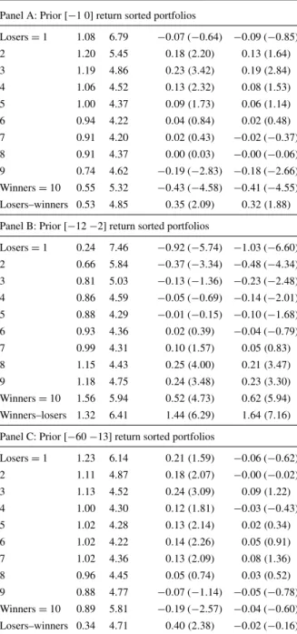
The anomalies based on returns pose a significant challenge not only to CAPM but to the efficient markets hypothesis, originally proposed by Fama (1970). Since they require knowledge of only past prices, they violate even the weak-form of market ef-ficiency. Table2shows the results of short-term reversal, medium-term momentum, and long-term reversal portfolios using US stocks over 1946 to 2010. In addition to CAPM alphas, I also show Fama and French’s (1993) three-factor alphas (this model is discussed later in Sect.3.2.3). The difference in returns between winners and losers is−0.53, 1.32, and−0.34% for stocks sorted on past month, past 2 to 12 months, and past 13 to 60 months returns, respectively. These differences in returns are, in general, not explained by risk factors. One-factor alphas are similar in magnitude to excess returns. Three-factor alphas show modest mispricing for short-term rever-sal but subsume completely the long-term reverrever-sal. In contrast, three-factor alphas for medium-term momentum portfolios are even larger than one-factor alphas. The magnitude of alphas for the long-short winners–losers portfolio is astounding 1.64%. Fama (1998) and Fama and French (2008) concede momentum as posing the biggest challenge to efficient markets hypothesis.
Accounting-based ratios There is also a vast literature that uses primarily account-ing-based information to predict the cross section of returns. Lakonishok et al. (1994) find a negative relation between returns over long horizon and financial performance such as earnings and sales growth. La Porta (1996) shows that analysts’ long-run earnings growth forecasts are negatively related to future returns. Haugen and Baker (1996) and Cohen et al. (2002) find that more profitable firms have higher returns than less profitable firms.
There have also been studies of the relation between investments and stock returns with mixed results. Chan et al. (2001) report that there is no difference in returns between firms doing R&D and those doing no R&D. However, amongst the firms engaged in R&D, high R&D expenditure relative to market value of equity signals high future excess returns. Titman et al. (2004), however, find that firms that invest more have lower stock returns. Cooper et al. (2008) report that firms with high asset growth have low returns; Lipson et al. (2010) show that this anomaly is stronger with in stocks with higher idiosyncratic volatility. Titman et al. (2010) and Watanabe et al. (2011) show that asset-growth anomaly exists in international markets too.
Sloan (1996) shows that accounting accruals are negatively related to returns sug-gesting that investors are unable to distinguish between accounting income and cash flows. Frankel and Lee (1998) show that residual-income based valuation models
Table 2 Past return sorted
portfolios. Stocks are sorted monthly into portfolios based on prior returns (further details on portfolio construction are on Ken French’s website). The table reports average returns, standard deviation of returns, and CAPM and Fama and French (1993) three-factor alphas. All returns and alphas are in percent per month and the correspondingt-statistics are in parentheses. The sample includes all US stocks. The sample period is 1946 to 2010
Decile Mean Std. dev. Alpha1 Alpha3
Panel A: Prior[−1 0]return sorted portfolios
Losers=1 1.08 6.79 −0.07(−0.64) −0.09(−0.85) 2 1.20 5.45 0.18(2.20) 0.13(1.64) 3 1.19 4.86 0.23(3.42) 0.19(2.84) 4 1.06 4.52 0.13(2.32) 0.08(1.53) 5 1.00 4.37 0.09(1.73) 0.06(1.14) 6 0.94 4.22 0.04(0.84) 0.02(0.48) 7 0.91 4.20 0.02(0.43) −0.02(−0.37) 8 0.91 4.37 0.00(0.03) −0.00(−0.06) 9 0.74 4.62 −0.19(−2.83) −0.18(−2.66) Winners=10 0.55 5.32 −0.43(−4.58) −0.41(−4.55) Losers–winners 0.53 4.85 0.35(2.09) 0.32(1.88)
Panel B: Prior[−12−2]return sorted portfolios
Losers=1 0.24 7.46 −0.92(−5.74) −1.03(−6.60) 2 0.66 5.84 −0.37(−3.34) −0.48(−4.34) 3 0.81 5.03 −0.13(−1.36) −0.23(−2.48) 4 0.86 4.59 −0.05(−0.69) −0.14(−2.01) 5 0.88 4.29 −0.01(−0.15) −0.10(−1.68) 6 0.93 4.36 0.02(0.39) −0.04(−0.79) 7 0.99 4.31 0.10(1.57) 0.05(0.83) 8 1.15 4.43 0.25(4.00) 0.21(3.47) 9 1.18 4.75 0.24(3.48) 0.23(3.30) Winners=10 1.56 5.94 0.52(4.73) 0.62(5.94) Winners–losers 1.32 6.41 1.44(6.29) 1.64(7.16)
Panel C: Prior[−60−13]return sorted portfolios
Losers=1 1.23 6.14 0.21(1.59) −0.06(−0.62) 2 1.11 4.87 0.18(2.07) −0.00(−0.02) 3 1.13 4.52 0.24(3.09) 0.09(1.22) 4 1.00 4.30 0.12(1.81) −0.03(−0.43) 5 1.02 4.28 0.13(2.14) 0.02(0.34) 6 1.02 4.22 0.14(2.26) 0.05(0.91) 7 1.02 4.36 0.13(2.09) 0.08(1.36) 8 0.96 4.45 0.05(0.74) 0.03(0.52) 9 0.88 4.77 −0.07(−1.14) −0.05(−0.78) Winners=10 0.89 5.81 −0.19(−2.57) −0.04(−0.60) Losers–winners 0.34 4.71 0.40(2.38) −0.02(−0.16)
generate a value-price ratio that has predictive power for future returns. Lee et al. (1999) use this valuation model to calculate the intrinsic value of Dow 30 stocks.
There is also a relation between firm financing decisions and stock returns. Loughran and Ritter (1995) show that stock returns are negative after equity issuances
and Ikenberry et al. (1995) show that repurchases generally result in positive stock returns. Daniel and Titman (2006) and Pontiff and Woodgate (2008) combine these pieces of evidence to show a negative relation between net stock issues and future stock returns.
Finally, there is very old literature going back to Ball and Brown (1968) who show that stock prices continue to drift in the direction of earnings surprises for several months after the earnings are announced. Bernard and Thomas (1989,1990) show that this anomaly is still robust after its initial discovery, although Chordia et al. (2009) show that this anomaly is prevalent in only illiquid stocks. Womack (1996) shows that stock prices also drift in the direction of analysts’ revisions and Sorescu and Subrahmanyam (2006) show that the drift occurs only for experienced analysts. Idiosyncratic-risk based ratios A central tenet of asset pricing models is that only systematic risk gets compensated. Nevertheless, there are several asset pricing models that take idiosyncratic risk into account. Levy (1978), Merton (1987), and Malkiel and Xu (2002) build extensions of the CAPM where investors, for some exogenous reason, hold undiversified portfolios.
Early research, for example Fama and MacBeth (1973), finds no support for pric-ing of idiosyncratic risk. However, Lehmann (1990) reaffirms the results of Douglas (1969) after conducting a careful econometric analysis. Malkiel and Xu (1997,2002) also present evidence of the importance of idiosyncratic risk in explaining the cross section of expected stock returns, even after controlling for size. In more recent work, Ang et al. (2006,2009) present evidence that stock returns are negatively related to idiosyncratic risk. Their study is interesting because not only it shows a relation be-tween idiosyncratic risk and return but also the relation goes the other way than that would be suggested by basic risk-return trade-off.
However, this study has been controversial. Bali and Cakici (2008) find that minor variations in research design invalidate the main findings. Huang et al. (2010) show that return reversals over one month are the major reason for the negative relation between idiosyncratic volatility and returns. In a twist, Fu (2009) shows that alterna-tive volatility calculations lead to a posialterna-tive relation between idiosyncratic volatility and returns. Finally, in a comprehensive analysis, Fink et al. (2011) show that there is indeed a positive relation between idiosyncratic volatility and returns but only if the investors know all the parameters of the model used to calculate idiosyncratic volatil-ity. They also show that there is no relation between idiosyncratic volatility forecasts made using real-time data and future returns, invalidating the use of this anomaly for a trading strategy.
3.2.2 Anomalies based on liquidity and trading frictions
Most of the asset pricing models assume frictionless markets. Trading costs are, how-ever, of course, an integral part of the investment process. The literature on incorpo-rating trading frictions in theoretical models as well as empirical studies was slow to pick up. The recent financial crisis has highlighted the importance of liquidity in the functioning of capital markets. This has given a huge impetus and liquidity has become an area of active research.
Liquidity as a characteristic The returns realized by investors are net of trading costs. This implies that stocks with higher trading costs should command higher re-turns to compensate for their lack of liquidity. Amihud and Mendelson (1986) pioneer this concept of liquidity being priced in stock prices. They document that there is a premium for bid–ask spread in stock returns. Liquidity is, however, multifaceted and different authors use different measures of liquidity. Datar et al. (1998) and Brennan et al. (1998) find that turnover as a proxy for liquidity is negatively related to future stock returns. Brennan et al. (2010) find that the effect of illiquidity is primarily from the sell-side. One of the most commonly used indicators of (il)liquidity is the one proposed by Amihud (2002) and is measured as the ratio of absolute return to dollar trading volume. Hasbrouck (2009) presents evidence of pricing of various, but not all, liquidity measures.
Liquidity as risk A parallel literature studies whether liquidity is a priced risk fac-tor. Acharya and Pedersen (2005) provide a useful taxonomy of various components of liquidity risk. First, there maybe commonality in liquidity, the covariance between individual stock liquidity and market liquidity. Chordia et al. (2000), Hasbrouck and Seppi (2001), and Huberman and Halka (2001) document the existence of commonal-ity in liquidcommonal-ity in the US stock market. Second, risk might arise due to the covariance between individual stock return and market liquidity. Pástor and Stambaugh (2003) measure illiquidity by the extent to which returns reverse high volume to capture this notion of liquidity and find that exposure to this liquidity risk is related to expected re-turns. Third, the covariance between individual stock liquidity and market return also leads to liquidity premium. Brunnermeier and Pedersen (2009) propose a theoretical model to consider the relationship between asset liquidity and funding availability in the stock market. Korajczyk and Sadka (2008) examine various liquidity measures and find that common component of these measures is a priced factor. At the same time, liquidity is also priced as a characteristic.
Information risk There is also a literature on the pricing of information risk. Easley and O’Hara (1987) develop a model where the probability of informed trading (PIN) is related to trading costs and stock returns. Easley et al. (1996), Easley et al. (2002), and Easley and O’Hara (2004) find support for the pricing of PIN in the cross section of stock returns. However, Duarte and Young (2009) report that it is only the liquid-ity trading component of PIN, rather than the information-based component, that is priced. Hou and Moskowitz (2005) find that one minus theR2from a market model regression is related to the cross section of stock returns. These authors interpret their measure capturing information asymmetry.
Short selling Miller (1977) proposes that stocks with short-sale constraints that will be overvalued as investors with negative outlook have a lower bound of zero on the number of shares that they can own. Jones and Lamont (2002) show that short-stock-rebate rate is a good proxy for short sale constraints and stocks with this high cost of borrowing have low future returns. Desai et al. (2002) find statistically significant subsequent underperformance for heavily shorted firms. Asquith et al. (2005) show that stocks with high short interest and low institutional ownership (the authors argue
that both these need to be present for a stock to be short sale constrained) earn low returns.
Diether et al. (2002) find that returns of stocks with higher dispersion of analysts’ earnings forecasts are lower; the effect is more pronounced for small firms, high book-to-market firms, and low momentum firms. The authors interpret their finding to be consistent with Miller. However, Boehme et al. (2006) argue that both difference in opinion and short-sale constraints are necessary preconditions of Miller’s model. The authors report evidence of significant overvaluation for stocks that are subject to both conditions simultaneously.
On a related topic, some studies examine the role of stock ownership in explaining the cross section of returns. Chen et al. (2002) show that stocks with an increase in breadth of ownership have higher returns than those with a decrease in breadth of ownership. This is consistent with the view that short sales are less binding when there are more investors with long positions. Nagel (2005) shows that stocks with high degree of institutional ownership have less cross-sectional predictability and exhibit more efficient pricing.
3.2.3 Factor models inspired by anomalies
I have already discussed liquidity-based factor models in Sect.3.2.2. In this section, I review the most famous three-factor model of Fama and French (1993) and its four-factor successor.
Three-factor model The interpretation of Fama and French (1992) study has been the subject of considerable controversy. The first possibility is that the results are spurious and due to data mining. However, Chan et al. (1991) show the B/M effect in Japan; Capaul et al. (1993) show a similar effect in four European markets and Japan; Fama and French (1998) document evidence of price-ratio based returns for twelve non-US major markets and emerging markets. More recently, Hou et al. (2011) and Fama and French (2011) provided more comprehensive and up-to-date evidence of size- and value-effects in international markets. Davis et al. (2000) provide an out-of-sample study for the US market itself by extending the sample period back to 1927. These studies suggest that price-ratio based anomalies are not specific to the US and/or a sample period.
Another explanation for the price-ratio based anomalies is rooted in behavioral theories. Lakonishok et al. (1994) argue that investors overreact. Since stocks with high B/M ratios are typically those that have fallen on hard times, investors irra-tionally extrapolate this performance resulting in too low prices for these stocks and too high prices for low B/M stocks. The future pattern of returns is just a correction for this overreaction.
Fama and French (1993) propose a three-factor model to rationalize these anoma-lies. They show that two new factors (SMB and HML) in addition to the usual market factor are useful for explaining the cross section of returns. The SMB factor is meant to capture the covariation of returns with size while the HML factor captures the co-variation of returns with book-to-market. Figure1plots the relation between actual returns and those predicted by CAPM (Panel A) and the three-factor model (Panel B)