Aus dem Institut für Centrum für Schlaganfallforschung Berlin. der Medizinischen Fakultät Charité Universitätsmedizin Berlin DISSERTATION

(1)

Aus dem Institut für Centrum für Schlaganfallforschung Berlin

der Medizinischen Fakultät Charité – Universitätsmedizin Berlin

DISSERTATION

Exploring Novel Magnetic Resonance Imaging Markers for Ischemic

Stroke in the Application of Vessel Size Imaging and Amide Proton

Transfer Imaging

zur Erlangung des akademischen Grades

Doctor of Philosophy (PhD)

im Rahmen des

International Graduate Program Medical Neurosciences

vorgelegt der Medizinischen Fakultät

Charité – Universitätsmedizin Berlin

von

Chao Xu

aus Hebei, China

(2)

Gutachter: 1. PD. Dr. med. Jochen B. Fiebach

2. Prof. Dr. rer. nat. habil. Harald E. Möller

3. Prof. Dr. rer. nat. Ingolf Sack

(3)

List of Abbreviations

3D three-dimensional

ADC apparent diffusion coefficient AIF arterial input function APT amide proton transfer APTR amide proton transfer ratio ASL arterial spin labelling CA contrast agent

CBF cerebral blood flow CBV cerebral blood volume

CEST chemical exchange saturation transfer CSF cerebrospinal fluid

DNR diffusional narrowing regime DSC dynamic susceptibility contrast DWI diffusion-weighted imaging EPI echo planar imaging FID free induced decay

FLAIR fluid attenuation inversion recovery FLASH turbo fast low angle shot

FWHM full-width at half-maximum GE gradient echo

GM gray matter

HEA healthy tissue IGR infarct growth INF initial infarct IPE ischemic penumbra IQR interquartile range

(11)

ix MRI magnetic resonance imaging

MT magnetic transfer MTR magnetic transfer ratio MTT mean transit time MVD microvessel density

NMR nuclear magnetic resonance OLI oligemic area

PI perfusion imaging ppm parts per million RF radio frequency RD relative dispersion

ROC receiver operating characteristic ROI region of interest

SAR specific absorption rate SDR static dephasing regime

SE spin echo

SNR signal-to-noise ratio

ssCE-MRI steady-state susceptibility contrast-enhanced magnetic resonance imaging

TE echo time

TI invention time

Tmax time to reach the maximum

TOAST trial of Org 10172 in acute stroke treatment TOF time-of-flight

t-PA tissue plasminogen activator

TR repetition time TTP time to the peak VOI voxel of interest VSI vessel size index WM white matter

(12)

(13)

Chapter 1 Introduction

Stroke is a life-threatening disease that causes 9% of all deaths around the world [1]. About 87% stroke is caused by ischemia [1], which can be treated with the thrombolytic therapy within a narrow time window to restore the blood perfusion [2–4]. This treatment requires an accurate patient selection due to the risk of causing haemorrhage [5]. There-fore, developments of diagnostic methods for locating the ischemic region and assessing the severity are of great interest in stroke research.

Since introduced in 1973 [6], magnetic resonance imaging (MRI) has become one of the most important imaging techniques in modern radiology due to its invasive and non-radioactive methodology. Its usage in acute stroke management has widely and rapidly increased during the last decades due to its capability of early detection of ischemic lesions in multiple modalities, such as perfusion imaging (PI) [7] and diffusion-weighted imaging (DWI) [8]. Nowadays, clinicians employ the PI-DWI mismatch [9–12] to approximate the ischemic penumbra, which is the tissue at risk of infarction but still being salvageable [13]. However, this mismatch concept is challenged by the recoverable acute diffusion lesion and the overestimation of the ischemia in PI [14–17].

Two MRI techniques have been recently reported to provide novel imaging markers in the brain: 1) vessel size imaging, estimating the microvessel density (MVD) [18] and the mean vessel size [19, 20]; 2) amide proton transfer (APT) imaging, providing a pH-weighted contrast [21]. Both of them demonstrate the potential in describing pathologies of cerebrovascular diseases. However, neither of them has so far been utilized in the clinical stroke application.

(14)

2 CHAPTER 1. INTRODUCTION

Given that ischemia is a complex and multi-factored process, pathological changes of the microvasculature and the metabolic mechanism are expected in the ischemic tissue [22– 24]. Therefore, this work aims at the development of vessel size imaging and APT imaging in clinical stroke application, as well as the evaluation of the corresponding imaging markers for penumbra description.

This thesis is structured in five parts:

In the first part Background and Motivation, principal concepts of MRI, which are involved in this study, are covered in Chapter 2. Fundamental knowledge of ischemic stroke, such as its causes, classification and pathophysiology is introduced in Chap-ter 3. The current stroke MRI techniques, as the powerful diagnostic tool to identify the ischemic penumbra, are reviewed in Chapter 4 according to the on-going 1000Plus study performed in our imaging center (Center for Stroke Research Berlin at the Campus Benjamin Franklin of the Charit´e University Hospital Berlin). Chapter 5 addresses the motivation of this work for a better description of the ischemic penumbra.

The second part Vessel Size Imaging describes first the state of the art of this tech-nique in Chapter 6. Chapter 7 demonstrates the feasibility of this techtech-nique in clinical acute stroke studies by applying it in healthy subjects and a small patient cohort. The contribution of this technique in ischemic stroke research is evaluated in a group study in Chapter 8.

The third partNew Concept on Dynamic Susceptibility Contrast Imaging demon-strates an extended work about an observation during the study of vessel size imaging, which is a hysteresis loop formed by the dynamic changes of transverse relaxation rates during the passage of the contrast agent (CA) bolus through the vasculature. This ob-servation is introduced in Chapter 9. The formation of the loop is studied in Chapter 10 by simulating nuclear magnetic resonance (NMR) signals in a vascular tree model. To characterize the shape and the direction of the loop, Chapter 11 proposes an imaging marker and demonstrates its potential usage in cerebrovascular diseases.

The other novel imaging technique Amide Proton Transfer Imagingis introduced in the fourth part. The background of this technique, as well as its limitation in clinical ap-plication, is described in Chapter 12. The development of a pulse sequence with embedded field map and its preliminary application in subacute stroke patients are demonstrated

(15)

3 in Chapter 13.

The final partSummary and Outlooksummarizes the current work in Chapter 14 and gives an outlook of further research topics in Chapter 15.

(16)

(17)

Part I

Background and Motivation

(18)

(19)

Chapter 2 Magnetic Resonance Imaging

MRI is a medical imaging technique used in radiology to visualize detailed internal struc-tures by making use of the property of NMR to image nuclei of atoms inside the body. In this chapter, we briefly introduce the fundamental concepts of the NMR [25, 26] and the basic MRI sequence schemes [27, 28] to cover the background knowledge of MRI referenced in the following chapters. We note that the NMR physics introduced in this chapter is based on the classical Bloch formalism without including the interpretation in quantum mechanics.

2.1 Fundamental Concepts of Nuclear Magnetic

Res-onance

NMR is a physical phenomenon in which magnetic nuclei in a magnetic field absorb and re-emit electromagnetic radiation. In the biological tissue with large content of water molecules, the NMR of the protons in hydrogen atoms (1_{H) contributes to the contrast}

of MRI.

2.1.1 Proton Spins and Magnetization

A proton spinning around its axis results in an intrinsic magnetic dipole moment ~µ. It also interacts with an external magnetic field B~0 to experience the precession about the

(20)

8 CHAPTER 2. MAGNETIC RESONANCE IMAGING

Figure 2.1: By definition, precession is the circular motion of the axis of rotation of a spinning body about another fixed axis caused by the application of a torque in the direction of the precession. The interaction of the proton’s spin with the magnetic field produces the torque, causing it to precess aboutB~0 as the fixed axis. Figure is modified from [28].

direction of the field (see Fig. 2.1). The precession angular frequency for the proton magnetic moment is given by

ω0 =γB0, (2.1)

where ω0 is referred to as the Larmor frequency, and γ is the constant named as the

gyromagnetic ratio. The hydrogen proton in water has a γ of 2.68×108 _{rad/s/T, which}

results in a Larmor frequency of 127.8 MHz for a 3 T magnetic field. The magnetic moment vector for a spin aligns in either parallel (lower energy) or anti-parallel (higher energy) direction along the external magnetic field due to thermal energy kT, where k is the Boltzmann’s constant and T is the absolute temperature. The number of spins in a parallel alignment exceeds that in an anti-parallel alignment with a fraction of ¯hω0/2kT

in the total number of spins in the sample. Here, ¯h≡h/(2π) is in terms of the Planck’s quantum constanth. Although the fraction of spin excess is in the order of one in millions, it is enough to achieve a significant magnetizationM~ per unit volume as the composition of all the spin moment vectors as

~ M = 1 V X i ~ µi (2.2)

in a macroscopic sample sizeV because of the large abundance of spins in biological tissue. For a sample with a spin density of ρ0, the longitudinal equilibrium magnetization M0

(21)

2.1. FUNDAMENTAL CONCEPTS OF NMR 9 along the external field B~0 direction is given by

M0 =

ρ0γ2¯h2

4kT B0. (2.3)

2.1.2 Relaxation

Similar to the effect of the gravitational field on a spinning top, the torque on a macro-scopic magnetizationM~ due to an external magnetic fieldB~ follows the differential equa-tion

d ~M

dt =γ ~M×B,~ (2.4)

if no interaction between spins and the neighbourhood environment is considered. Eq. (2.4) can be separated into two decoupled equations for a longitudinal magnetization compo-nent Mz parallel to the external magnetic field B~ and a transverse magnetization com-ponentM⊥ in the plane perpendicular to B~:

dMz dt = 0, (2.5) d ~M⊥ dt =γ ~M⊥× ~ B. (2.6)

Interactions of protons with their neighbourhood lead to additional terms in Eq. (2.4), which are discussed as follows.

Introduction of T1

A macroscopic magnetization M~ that has been tilted by a radio frequency (RF) pulse in a static field will return to its macroscopic statistical equilibrium M0. This process

is called “spin-lattice relaxation”. Nuclei held within a lattice structure are in constant vibrational and rotational motion, creating a complex magnetic field. The magnetic field caused by thermal motion of nuclei within the lattice is called the lattice field. The lattice field of a nucleus in a lower energy state can interact with nuclei in a higher energy state, causing the energy of the higher energy state to distribute itself between the two nuclei. Therefore, the energy gained by nuclei from the RF pulse is dissipated as increased vibration and rotation within the lattice, which can slightly increase the

(22)

temperature of the sample. The rate of change of the longitudinal magnetization Mz can be characterized by a empirically-determined constant referred as the longitudinal relaxation rate R1. Its inverse T1 ≡ 1/R1 is the experimental longitudinal relaxation

time. So the component Mz in Eq. (2.5) takes the form of

dMz

dt =

1

T1

(M0−Mz), (2.7)

where M0 is the equilibrium magnetization.

Introduction of T2

The mechanism that the transverse magnetization M⊥ decays towards its equilibrium

value of zero due to the dephasing of spins is called “spin-spin relaxation”. The same mechanism that is active in spin-lattice relaxation is active for spin-spin relaxation. Ad-ditionally, spins interact with each other through coupling or chemical exchange. During the spin-spin relaxation, the individual spins dephase with time and thus reduce the net magnetization vector. The rate of reduction in transverse magnetization is characterized by another experimental parameter R2, referred to as the transverse relaxation rate. Its

inverse T2 ≡ 1/R2 is named as the transverse relaxation time. The differential equation

in terms of the transverse magnetization M⊥ is changed by the addition of term with a

transverse relaxation time as

d ~M⊥ dt =γ ~M⊥× ~ B− 1 T2 ~ M⊥. (2.8) Introduction of T₂∗ and T₂0

In practice, there are additional dephasing mechanisms affecting the transverse relaxation in biological tissue. First, spins at different positions in a sample may experience different field strength. The magnetic field inhomogeneity can be either due to a variation of the static magnetic field, or induced by biological tissue structures, such as blood vessels and nerve fibres. This decay is principally reversible by RF rephasing if spins stay within the same scale of field strength before and after the RF refocusing. On the other hand, spins may diffuse to other places in a magnetic gradient field. This decay is irreversible since

(23)

2.2. IMAGING TECHNIQUES 11 it is impossible to restore the position of spins.

The decay of magnetization affected by field inhomogeneity and diffusion is characterized by a rateR0₂. So the total effective relaxation rate, defined as R₂∗, is the sum of the spin-spin interaction relaxation rate and the additional relaxation rate as

R₂∗ =R2+R02. (2.9)

Its inverse T₂∗ ≡1/R∗₂ takes the form of 1 T₂∗ = 1 T2 + 1 T₂0. (2.10) Bloch Equation

The differential Eqs. (2.7) and (2.8) can be combined into one vector equation as

d ~M dt =γ ~M⊥× ~ B+ 1 T1 (M0−Mz) ˆz− 1 T2 ~ M⊥, (2.11)

which is referred to as the Bloch equation. For a constant field case B~ = B0zˆ, the

corresponding solutions in a rotation frame about z-axis with the Larmor frequency are

Mz(t) =Mz(0)e−t/T1 +M0 1−e−t/T1

, (2.12)

M⊥(t) =M⊥(0)e−t/T2. (2.13)

2.2 Imaging Techniques

2.2.1 Gradient Echo and

T

₂∗

The simplest MRI experiment can be done by the application of a 90◦ RF pulse to rotate the longitudinal magnetizationM0 into the transverse plane and the measurement of the

(24)

Figure 2.2: Sequence schemes of basic (A) gradient echo (GE) and (B) spin echo (SE) sequences. TE indicates the echo time; RF, radio-frequency pulse; SS, slice selection; PE, phase encoding; RO, readout.

According to Eq. (2.13), the recorded signal in the rotation frame takes the form of

M⊥(t) = M0e−t/T

∗

2. (2.14)

We note that the relaxation is characterized by T₂∗ rather than T2, since magnetic field

inhomogeneities affect the decay in practice.

A gradient echo (GE) is generated by using a pair of bipolar gradient pulses. In Fig. 2.2A, the basic GE sequence is illustrated. The data are sampled during a GE, which is achieved by dephasing the spins with a negatively pulsed gradient before they are rephased by an opposite gradient with opposite polarity to generate the echo. Essentially, the signal acquired corresponds to the FID, as the echo producing gradients only compensate for the applied imaging gradients.

In an MRI experiment, the scheme in Fig.2.2A is played repeatedly to acquire multiple lines in k-space with an interval of repetition time (TR), so that the start magnetiza-tion for FID from the second TR on is M0 1−e−TR/T1

instead of M0. Therefore, the

magnetization vector contributing to the GE is

M⊥(TE) = M0 1−e−TR/T1

e−TE/T2∗_, _(2.15) where TE is the echo time. For a long TR (relative to T1) and TE comparable with

T₂∗, the image is weighted by both spin density and T₂∗. The contrast between tissues with different T2 is enhanced. For a sequence with such parameter settings, we call it

(25)

2.2. IMAGING TECHNIQUES 13

T₂∗-weighted imaging. Its usage in stroke research is introduced in Section 4.2.2.

2.2.2 Spin Echo

A spin echo (SE) sequence is illustrated in Fig. 2.2B. The 90◦ excitation pulse rotates the longitudinal magnetization into the xy-plane and the dephasing of the transverse magnetization M⊥ starts. The following application of a 180◦ refocusing pulse generates

signal echoes. The purpose of the 180◦ pulse is to rephase the spins, causing them to regain coherence and thereby to recover the transverse magnetization, producing an SE. A multiple SE experiment (e.g. Carr-Purcell-Melboom-Gill sequence [29, 30]) applying multiple 180◦ pulses after a single 90◦ pulse can be a way to approach the intrinsic T2, if

the refocusing is effective over the whole sample and the irreversible dephasing caused by spatial diffusion of spins is minimized. This condition is hard to achieve since it requires the exact performance of RF pulses and the minimized inter-echo time. Therefore, the measured SE relaxation time T2SE is shorter than the intrinsic T2 and depends on the

sequence parameters used in the experiment.

2.2.3 Inversion Recovery

The inversion recovery experiment produces imaging contrasts sensitive to T1. The

ap-plication of an initial 180◦ inversion pulse before a basic GE or SE sequence (see Fig. 2.3) rotates the longitudinal magnetization first into the negative ˆz direction, so that Mz starts with a negative of the equilibrium value

Mz(0) =−M0. (2.16)

The inversion time (TI) is defined as the time between the inversion pulse and the 90◦ excitation pulse. The magnetization regrows to its equilibrium value in the interval ofTI according to Eq. (2.12)

Mz(t) =M0 1−2e−t/T1

(26)

Figure 2.3: The diagram of inversion recovery sequence. RF indicates the radio frequency pulses; SS, slice selection; PE, phase encoding; RO, readout; TI, inversion time.

After the longitudinal magnetization is tipped into the transverse plan to provide the initial signal, the magnitude of the transverse magnetization evolves as

M⊥(t) =

M₀ 1−2e−TI/T1

e−(t−TI)/T2, whent > T_I. (2.18)

We note that the factor M0 1−2e−TI/T1

is zero if TI is selected as

TI =T1ln 2. (2.19)

For a uniform sample, T1 can be precisely measured by varying TI to achieve a zero in signal.

2.3 Magnetic Properties of Tissue and Contrast Agents

The magnetic susceptibilityχis an intrinsic property of a material, which is the degree of magnetization of a material in response to a magnetic field. Susceptibility variations in body tissue and exogenous CAs can be useful in contributing imaging contrasts in MRI. All materials have induced dipole moments in the presence of external magnetic fields. The electrons pair up to cancel their spin magnetic moments. This effect is called dia-magnetism. The macroscopic sum of the induced moments is roughly anti-parallel to the external magnetic field, so that its associated macroscopic field weakly opposes the external field. The susceptibility is negative χ <0 for diamagnetic materials.

(27)

2.3. MAGNETIC PROPERTIES OF TISSUE AND CA 15 An atom with an unpaired electron has a non-vanishing permanent magnetic moment with an associated non-zero dipole magnetic field. Those atom moments in a material would tend to align with an external magnetic field, producing a bulk magnetic moment and a corresponding macroscopic magnetic field augmenting the external field. This effect is referred to as paramagnetism, which is a much stronger effect than diamagnetism. The susceptibility is positive χ >0 for paramagnetic materials.

Metal ions show a suitable paramagnetic effect which depends on the number of unpaired electrons in the ion. The Fe3+ _{and Gd}3+ _{ions are suitable candidates for a relaxation}

agent, since their electron-spin relaxation time matches the Larmor frequency of the protons (about 10−8 _{- 10}−10 _{s). A deoxyhemoglobin molecule consisting of a Fe}3+ _ion

with unpaired electrons is paramagnetic and is served as an endogenous CA in functional blood-oxygen-level dependence imaging [31]. Since free Gd3+ ions are extremely toxic, they are bound into a chelate complex in intravenous CAs for clinical use.

Paramagnetic CAs affect the MRI contrast in two ways: dipolar relaxation effects and susceptibility induced relaxation effects [32].

In the former process, the relaxation of tissue is enhanced by the dipole-dipole interaction between the free electron spins of the paramagnetic ion in a CA molecule and the proton spins in water [33]. A linear relationship between the CA concentration and the increase in relaxation rates [34, 35] can be defined in terms of the relaxivity of the CA as

R1 =R01+r1C, (2.20)

R2 =R02+r2C, (2.21)

where R0

1 and R02 are the relaxation rates without the presence of the CA,r1 and r2 are

the relaxivity constants of the CA, and C is the molar concentration of the CA.

The latter process can be understood as the magnetic field inhomogeneity induced by a paramagnetic CA. The induced magnetic field B~i of a material in an external magnetic field B~0 is

~

Bi = (1 +χ)B~0. (2.22)

Therefore, a paramagnetic CA with a susceptibility change ∆χ compared to the sur-rounding tissue will induce a local field difference of ∆B = ∆χB0. This leads to a shift

(28)

of Larmor frequency

∆ω =γ∆χB0, (2.23)

and thus shortens T2/T2∗ with a consequent dephasing of spins during the transverse

(29)

Chapter 3 Ischemic Stroke

A stroke is the rapidly developing loss of brain functions due to the disturbance in the blood supply to the brain, and causes 9% of all deaths around the world as the second most common cause of death after ischemic heart disease [1]. Stroke can be either ischemic or haemorrhagic (see Fig. 3.1). Ischemic strokes are those that are caused by interruption of the blood supply, while haemorrhagic strokes are the ones which result from the rupture of a blood vessel or an abnormal vascular structure. About 87% of strokes are caused by ischemia [1]. In this chapter, we review the fundamental knowledge of ischemic stroke, such as its causes, classification and pathophysiology.

3.1 Causes and Classification

Cerebral ischemia is a restriction of the blood supply to the brain, leading to the dys-function and death of the brain tissue. The restriction of the blood can be thrombosis or embolism.

The thrombosis is the obstruction of a blood vessel by a thrombus forming locally in an artery directly leading to the brain. The thrombosis can arise from the large vessels (e.g. the internal carotid artery, the vertebral artery and the circle of Willis), or the small arteries inside the brain (e.g. branches of circle of Willis and middle cerebral artery, and the arteries arising from the distal vertebral and basilar artery) [36]. In rare cases, the thrombosis originates from the dural venous sinuses, where the thrombus is formed due to the locally increased venous pressure exceeding the pressure generated by the

(30)

18 CHAPTER 3. ISCHEMIC STROKE

A

B

Figure 3.1: Subtypes of stroke: (A) ischemic and (B) haemorrhagic stroke. (A) Ischemic stroke is caused by the interruption of blood flow to the brain due to a clot, which stops the flow of the blood to the tissue. The shortage of oxygen and nutrients results in tissue damage. (B) Haemorrhagic stroke is caused by the rupture of a blood vessel or an abnormal vascular structure. Blood leaks into brain tissue and causes the cell death. Images are from the Heart and Stroke Foundation of Canada.

(31)

3.2. PATHOPHYSIOLOGY 19 arteries [37, 38].

The embolism is the blockage of an artery due to an embolus travelling in the arterial bloodstream originating from elsewhere of the body, most commonly from the heart. Emboli of cardiac origin are a frequent cause of large brain infarcts and haemorrhagic brain infarcts with often initial severe symptoms [39]. On the other hand, the embolism linked with the system hypoperfusion is associated with less severe clinical deficits. The borderzone infarction between the territories of two major arteries is often seen in this case [40].

The trial of Org 10172 in acute stroke treatment (TOAST) classification based mainly on the aetiology differentiates cerebral ischemia into large-artery atherosclerosis from em-bolus or thrombosis, cardioembolism, small-vessel occlusion, stroke of other determined aetiology and stroke of undetermined aetiology [36]. This classification aids clinicians to monitor the prognosis, the outcome and the management of stroke patients [41–43].

3.2 Pathophysiology

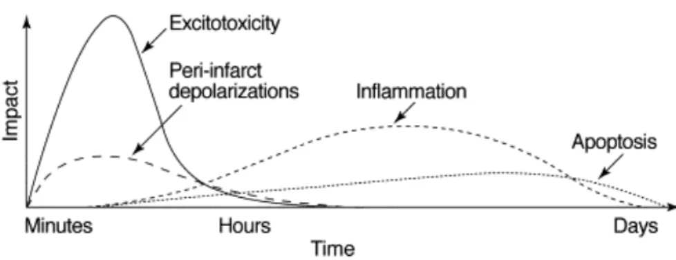
The reduction of blood flow and energy supply to the brain during ischemia triggers several mechanisms, which lead to cell death. The evolution of these pathophysiological processes spreads from hours to days (Fig. 3.2) and mediates the injury of neurons, glial cells and microvessels [23].

The first consequence of perfusion deficit is the depletion of oxygen and glucose, which causes the accumulation of lactate via anaerobic glycolysis. The acidosis modifies the activity of antioxidant enzymes, enhances the free-radical formation and worsens the brain injury by triggering the inflammation and the apoptosis [44–46].

Energy failure on Na+/K+ -ATPase and Ca2+/H-ATPase pumps leads to the elevation of intracellular Na+_{, Ca}2+ _{and Cl}− _{and the increase of extracellular K}+ _{[47]. This leads}

to the loss of the osmotic pressure and the cytotoxic edema consequently. The loss of the membrane potential results in the depolarization of neuron and glia. The excitotoxic amino acids, especially glutamate, are discharged into the extracellular space, which harm the neurons and cause the necrosis [23].

(32)

20 CHAPTER 3. ISCHEMIC STROKE

Figure 3.2: Putative cascade of damaging events in focal cerebral ischemia. Very early after the onset of the focal perfusion deficit, excitotoxic mechanisms can damage neurones and glia lethally. In addition, excitotoxicity triggers a number of events that can further contribute to the demise of the tissue. Such events include peri-infarct depolarizations and the more-delayed mechanisms of inflammation and programmed cell death. The x-axis reflects the evolution of the cascade over time, while the y-axis aims to illustrate the impact of each element of the cascade on final outcome. The figure is from [23].

Within minutes of occlusion, there occurs the upregulation of proinflammatory genes, which produces mediators of inflammation. After the expression of adhesion molecules at the vascular endothelium, neutrophils transmigrate from the blood into the brain parenchyma, followed by macrophages and monocytes [48]. Whereas the microvascular obstruction by neutrophils can worsen the degree of ischemia, production of toxic media-tors by activated inflammatory cells and injured neurons can amplify tissue damage [49]. All the pathological processes mentioned above trigger the apoptosis, which occurs par-ticularly in the tissue with milder ischemic injury, defined as ischemic penumbra (see Section 4.1). The apoptotic process can last for days after the ischemia onset and is mediated by two general signal pathways involving either the disruption of mitochondria or the activation of death receptors located on the plasma membrane [50].

Apart from the neuron injury, microvessels undergo the mechanical or hypoxic damage of vascular endothelium. Toxic damage of inflammatory molecules and free radicals, the destruction of the basal lamina by matrix metalloproteinases, and the compression of swollen astrocytic end-feet are potential causes of microvessel obstruction and blood-brain-barrier disruption during ischemia [24, 51].

(33)

Chapter 4 Stroke Magnetic Resonance Imaging

The delineation of ischemic penumbra from normal tissue and infarction at the acute stage is of great importance for targeting the patients for therapy and thus is the main focus of stroke imaging research. MRI techniques provide not only the early detection of ischemic lesion with high sensitivity, but also the capability of imaging the lesion with multi-modalities. Therefore, its usage has widely and rapidly increased in acute stroke management during the last decades. In this chapter, we review the concept of ischemic penumbra as an imaging diagnostic target and introduce the 1000Plus study performed in our imaging center, as well as the imaging sequences utilized in the protocols along this study.

4.1 Ischemic Penumbra

Within areas of severely reduced blood flow, which is termed as the core of the ischemic territory, excitotoxic and necrotic cell death occurs within minutes, and the tissue under-goes irreversible damage in the absence of prompt and adequate reperfusion [23]. How-ever, cells in the peripheral zones are supported by collateral circulation, and their fate is determined by factors including the severity of ischemia and the timing of reperfusion. In this peripheral region, termed as the ischemic penumbra, cell death occurs relatively slowly. This region is considered to be potentially salvageable [52]. However, the extent of penumbral tissue diminishes rapidly with time, thus the therapeutic time window is narrow [53]. The thrombolytic therapy, which is the intravenous tissue plasminogen

(34)

22 CHAPTER 4. STROKE MAGNETIC RESONANCE IMAGING

vator (t-PA), currently restricts the treatment window to 4.5 hours [54], since the delayed therapy increases the risk of haemorrhage [55]. The identification of ischemic penumbra for a better patient selection is thus of great importance in stroke research.

The most relevant definition of ischemic penumbra for clinical practice is based on neu-roimaging techniques. With the modern MRI techniques, the PI identifies the brain tissue with reduced blood perfusion and the DWI locates the severe ischemic core [10– 12, 56]. The PI-DWI mismatch regions indicate the ischemic penumbra, which serves as the target for thrombolytic therapy. Several clinical trials (the DIAS [57] and the DEDAS trial [58]) employing MRI to select patients on the basis of the PI-DWI mismatch have shown that patients treated in an extended time window have significantly higher rates of reperfusion and improved 90th day clinical outcome.

On the other hand, this mismatch concept is challenged by the observation that the DWI lesion may not be restricted to the infarct core [59] and the perfusion deficit often overestimates the final infarction [17, 60]. Furthermore, the definition of mismatch region is complicated by the selection of perfusion parameters [61], processing methods [62] and delineation thresholds [63–65]. Further investigations are certainly needed for profiling the mismatch concept. The on-going 1000Plus study performed in our stroke imaging center was designed to validate the PI parameter for infarct prediction and is introduced in the following Section 4.2.

Moreover, given that the ischemic tissue damage is complex and multi-factorial [23, 24], novel imaging markers can augment existing penumbral imaging and provide great in-sights into disease pathophysiology and perhaps, if validated, serve to help guide treat-ment decisions.

4.2 1000Plus Study

The 1000Plus study is an on-going trial designed as a prospective, single center observa-tional study conducted by our stroke imaging center to describe the incidence of mismatch and the predictive value of PI for final lesion volume depending on door-to-imaging time and vascular recanalization [66].

(35)

4.2. 1000PLUS STUDY 23

4.2.1 Study Design

The study aims to include 1200 patients and cover their MRI examinations from the acute stroke onset to one-week follow-ups. The inclusion criteria and study design are shown in Fig. 4.1.

All the examinations are performed with a 3 T MRI scanner (Tim Trio; Siemens AG, Erlangen, Germany). Our MRI protocol for acute stroke patients contains the following sequences for the day of admission (day 1) and day 2: T₂∗-weighted imaging to screen for intracerebral haemorrhage; DWI to assess cerebral infarction; time-of-flight magnetic resonance angiography (TOF-MRA) to detect vessel occlusion; fluid attenuation inversion recovery (FLAIR) to estimate microangiopathic lesions load and to investigate the age of the recent lesion; PI to determine the tissue at risk. On day 5 - 7, a third measurement with a shorter protocol excluding PI is performed to assess the final infarct size on FLAIR. An example of images obtained along the examination protocols is illustrated in Fig. 4.2. Each imaging technique involved in the 1000Plus study is described in detail as follows.

4.2.2 T

₂∗

-weighted Imaging

T₂∗-weighted imaging uses a basic GE sequence with aTE between the longest and shortest tissue T2 of interest and a long TR compared to T1. According to

M⊥(TE) =M0 1−e−TR/T1

e−TE/T2∗, (2.15) the contrast between tissue with different T₂∗s is enhanced. The T₂∗-weighted contrast is sensitive to susceptibility changes. The haemorrhage appears dark in T₂∗-weighted image due to the ferric iron deposition (see Fig. 4.2 on day 2 and day 6). The T₂∗-weighted imaging is performed in priority of other scans for exclusion of patients with bleeds for the thrombolytic therapy.

(36)

Figure 4.1: Study design and inclusion criteria of the 1000Plus Study. The figure is from [66]. ER indicates emergency room; CT, computer tomography; MRI, magnetic resonance imaging; DWI, diffusion-weighted imaging; TOF-MRA, time-of-flight magnetic resonance angiography; FLAIR, fluid attenuation inversion recovery; mRS, modified ranking scale to assess functional recovery in randomized stroke trials.

(37)

Figure 4.2: Example of images from a patient (female, 85 years) included in the 1000Plus study. The patient had a right middle cerebral artery infarct, M1 artery occlusion and perfusion imag-ing (PI) - diffusion-weighted imagimag-ing (DWI) mismatch on day 1, haemorrhagic transformation in the infarction on day 2, and increased infarction volume on day 6. FLAIR indicates fluid attenuation inversion recovery; MRA, magnetic resonance angiography; MTT, mean transit time; D1, first day after symptom onset; D2, second day after symptom onset; D6, sixth day after symptom onset.

(38)

4.2.3 Time-of-Flight Magnetic Resonance Angiography

The TOF-MRA enables the delineation of the vessel lumen by using the blood flow effects [67]. The blood flow is assumed to be perpendicular to the imaging plane or volume in the case of a three-dimensional (3D) study. For TR shorter than the T1 of

the stationary spins within the slice, the signal will be reduced due to partial saturation effects. Blood flow in the vessel will move spins from outside the slice which have not been subjected to the spatially selective RF pulses into the imaging slice. These unsaturated or fully relaxed spins have full equilibrium magnetization, and therefore upon entering the slice will produce a much stronger signal than stationary spins assuming that a GE sequence is applied. This effect is referred to as inflow enhancement [68]. A 3D reconstruction is performed to extract the vessel lumen from the plane images [69].

4.2.4 Fluid Attenuation Inversion Recovery

The FLAIR pulse sequence is a derivative of the inversion recovery sequence illustrated in Fig. 2.3. The 180◦inversion pulse is attached prior to the 90◦ excitation pulse of an SE acquisition, so that the longitudinal magnetization rotates into the negative plane after the inversion pulse. According to Eq. (2.18), the transversal magnetization M⊥ recorded

at the time of TE is M⊥(TE) = M₀ 1−2e−TI/T1 e−(TE−TI)/T2, (4.1)

where TI is the inversion time. According to Eq. 2.19, the effects of the fluid from the resulting image can be removed by selecting an appropriate TI as

TI =T1CSF ln 2, (4.2)

where T1CSF is the T1 of the cerebrospinal fluid (CSF). The M⊥ of the CSF in Eq. (4.1)

is nulled.

This technique suppresses the signal of fluid, which appears very bright in a normal T2

contrast. Therefore, the lesions adjacent to the cerebral cortex and ventricles, which are normally covered by the CSF signal, are visible by the dark fluid technique. The FLAIR

(39)

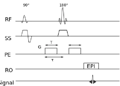
Figure 4.3: The diagram of an SE diffusion imaging sequence with the diffusion gradient (ampli-tude,G; duration, T) added in the phase-encoding direction. RF indicates the radio frequency pulses; SS, slice selection; PE, phase encoding; RO, readout; EPI, echo planar imaging.

sequence is widely used in detecting lesions with a long T2, for example, the vasogenic

edema surrounding a brain tumour [70, 71] and multiple sclerosis plaques [72] within the periventricular white matter. In stroke imaging, FLAIR images are used to identify the final infarction (see Fig. 4.2 on day 6).

4.2.5 Diffusion-weighted Imaging

The diffusion imaging sequence is able to measure the signal attenuation from the molec-ular motion in a certain direction by adding diffusion gradients to a basic sequence [73]. An example of the SE diffusion imaging sequence measuring the diffusion in the phase-encoding direction is shown in Fig. 4.3 with the gradient amplitude ofGand the duration ofT. According to the diffusion theory, the protons following the random walk will bring the signal decay as

S(G) =S(0)e−bD, (4.3) where S(G) is the MRI signal intensity with the amplitude of the diffusion gradient G,

S(0) is the MRI signal density without performing the diffusion gradient, and D is the diffusion coefficient. The gradient configuration factor b is defined as

(40)

Figure 4.4: Image modalities of diffusion imaging techniques in a stroke patient (female, 73 years) with right middle cerebral artery infarct. DWI indicates diffusion-weighted imaging; ADC, apparent diffusion coefficient; b, a gradient configuration factor described in Eq. (4.4) with the unit of s/mm2.

whereγ is the gyromagnetic ratio, and τ is the time from the start point of the diffusion gradient to the centerline of refocusing RF pulse.

Hence, the different coefficientD(x, y) in a certain direction (x, y) is obtain from a slope fitting as following:

D(x, y) = −1

b ln

S(x, y, G)

S(x, y,0), (4.5) where theS(x, y, G) indicates a diffusion-weighted signal in the direction of (x, y). In our imaging center, diffusion gradients were performed in six different directions with b = 1000 s/mm2_and_b_{= 0 s}_/_mm2 _{(Fig. 4.4). The magnitude of the vector}_D_~ _{is conventionally}

named as the apparent diffusion coefficient (ADC).

As described in Section 3.2, the membrane pumps become short of energy and stop functioning within minutes of ischemia. Osmotic pressure is consequently lost between the extracellular fluid and the cytoplasm. This results the movement of water from the extracellular space to the cells, which get swelling. The extracellular motion of water molecules is restricted due to the shortage of the extracellular space. This leads to a reduction of the ADC. Therefore, the ADC enables an early detection of the ischemic region, which appears a dark area in the ADC map (Fig. 4.4). Clinicians often employ diffusion-weighted images for lesion identification, since the ischemia is more recognizable as a clearly demarcated hyperintensity.

(41)

Figure 4.5: Illustration of process method in perfusion imaging in a patient (male, 78 years) with left internal carotid artery occlusion measured 20 hours after symptom onset. (A) Three echo planar imaging (EPI) images demonstrate the contrast change before, during, and after the bolus passage. (B) The curve of the signal intensity for comparison between the region of ischemic tissue and the contralateral healthy tissue. (C) The ∆R2 curve and the definition of

the parameter time to the peak (TTP).

4.2.6 Perfusion Imaging

In our imaging center, the dynamic susceptibility contrast (DSC) imaging is used to quantify the hemodynamic perfusion. It requires the injection of a bolus of the CA and employ a dynamic GE echo planar imaging (EPI) sequence to track the susceptibility-induced signal loss during the bolus passage through the brain (Fig. 4.5A) [74].

The change in transverse relaxation rate measured by GE ∆R2GE is converted from the raw MRI signal S(t) according to

∆R2(t) =− 1 TE lnS(t) S0 , (4.6)

where TE is the echo time and S0 is the baseline signal without CA injection.

According to Eq. (2.21), a linear dependence between the the change of transverse rate and the concentration of the CA inside the tissue Ct(t) is assumed, so that

(42)

Figure 4.6: Illustration of the definition of perfusion parameters. CBV indicates cerebral blood volume; CBF, cerebral blood flow; MTT, mean transit time; Tmax, time to reach the maximum.

where r is the relaxivity of the CA. The ∆R2GE curve can present as the scaled tracer-concentration curve, on which the time to the peak (TTP) is defined as the time from the starting point of the measurement to the peak of the curve (Fig. 4.5C).

If we know the arterial input function (AIF) to the brain Ci(t), which is manually or automatically selected from a voxel or from the averaged curve of several voxels, the tissue impulse response curve R(t) can be calculated by deconvoluting Ci(t) from the tracer-concentration curve Ct(t) according to

Ct(t) =f ·Ci(t)⊗R(t), (4.8) where f is the cerebral blood flow (CBF) [75]. Several perfusion parameters are defined on the scaled tissue impulse response curve R(t) after the deconvolution (see Fig. 4.6). The CBF is the maximum of the curve. The area under the curve is defined as cerebral blood volume (CBV). The time to reach the maximum (Tmax) shows the delay. The ratio between CBV and CBF is defined as mean transit time (MTT). The ischemic tissue demonstrate a decreased CBV and CBF, and a prolonged MTT and Tmax (Fig. 4.7), because the vessel blockage causes a delay and dispersion in blood transportation. All these parameters have been evaluated by clinicians to delineate the penumbra. How-ever, issues on the selection [61], the processing methods [62] and the delineation thresh-olds [63–65] of these perfusion maps are still under debate.

(43)

Figure 4.7: Perfusion maps of the patient shown in Fig. 4.5. TTP indicates time to the peak; Tmax, time to reach the maximum; MTT, mean transit time; CBV, cerebral blood volume; CBF, cerebral blood flow.

labelling (ASL), is also capable of the CBF estimation by using the endogenous CA, which is the magnetically labelled protons within water molecules in arterial blood before flowing to the imaged portion of the brain [76]. It measures the signal attenuation dependent upon the rates of the labelled spin flowing into the voxel and compares the contrast with a baseline image without labelling. Although ASL offers advantages over the CA injection and a potential absolute measurement of CBF, its intrinsic technical limitations causing a lower signal-to-noise ratio (SNR), longer measurement time and less resistance to patient motion compared to the DSC measurements restrict its current usages in acute stroke diagnosis [77–79].

(44)

(45)

Chapter 5 Motivation

An important focus of imaging research in the ischemic stroke is the differentiation of the ischemic penumbra from the infarct core and the normal tissue. Especially in patients presenting beyond the established time window of 4.5 hours after the stroke, in candidates for endovascular treatment, and in patients older than 80 years, a precise characterization of brain ischemia is required [80]. The mismatch between ischemic areas measured by PI and DWI has been considered to be a good approximation of the ischemic penumbra, yet it tends to overestimate it by containing regions of benign oligemia [17, 60] (Fig. 5.1). The overestimation afflicts the clinical routine as the final infarct volume is not predicted by the acute PI-DWI mismatch [11, 81]. Therefore, despite its widespread use at present, the PI-DWI mismatch is not a complete approach for imaging the penumbra [82–84]. As the thrombolytic therapy is accompanied by a considerable risk of haemorrhage, it is nec-essary to develop complementary imaging modalities that can characterize the ischemic penumbra in more detail.

Cerebral microvessels, which include capillaries, arterioles, and venules, express multiple dynamic responses to ischemia together with their neighbouring neurons [22]. The effects of ischemia on the microvasculature have so far mainly been described from the functional aspect [51, 85]. Because various vasomodulators are involved in this process [86–88], changes in microvascular morphology are apparently expected. Therefore, we hypothesize that the morphological variation of the microvascular network under ischemic conditions could be an effective way to describe the pathology of ischemic tissue and might provide useful information for describing the ischemic penumbra.

(46)

34 CHAPTER 5. MOTIVATION

Figure 5.1: The acute perfusion imaging (PI) - diffusion-weighted imaging (DWI) mismatch on day 1 overestimates the final infarction on day 6 in a patient (male, 78 years, left internal carotid artery occlusion, without recanalization). MTT indicates mean transit time; FLAIR, fluid attenuation inversion recovery.

Considering different orders between the common clinical imaging resolution in millime-ters and microvascular scale of micromemillime-ters, there is no way to image the microvascular network directly. Parameters reflecting properties of the local microvascular network in the imaging scale are used instead. Vessel size imaging, which provides a measure of MVD and a mean vessel size, was proposed as a novel approach to map the cerebral microvas-cular structure quantitatively [19]. Attempts have been made to apply this technique in animals stroke models [89, 90] and tumour patients [20, 91].

In this thesis, we aim to integrate vessel size imaging in clinical stroke study and evaluate the parameters provided by this technique in ischemic tissue.

As described in Section 3.2, the restriction of blood supply causes the immediate accu-mulation of lactate, which leads to the ischemic acidosis, i.e. a decrease in pH. The acidic environment modifies the activity of antioxidant enzymes, enhances the free-radical for-mation and causes the cell death. Therefore, tissue pH value may serve as an important physiological marker for the easy detection of the tissue at risk.

Although the lactate magnetic resonance spectroscopy is able to assess the tissue acidosis

in vivo [92], its spatial resolution is not yet appropriate for mapping the acute stroke patients. Recently, Zhou et al. [21] has proposed a technique, named amide proton transfer (APT) imaging, to differentiate the pH value by detecting the chemical exchange process between the amide protons in the mobile proteins and the protons in the water. This technique has so far demonstrated decreased pH values in the ischemic tissue of stroke rat brain [21, 93]. However, its usage is limited in clinical stroke studies due to

(47)

35 the strict time and the safety restriction of patient management.

As the second focus of our work, an APT imaging sequence is designed and implemented in the clinical scanner to overcome the technique limitation, and is applied to a pilot group of patients.

(48)

(49)

Part II

Vessel Size Imaging

(50)

(51)

Chapter 6 Vessel Size Imaging - State of the

Art

Vessel size imaging was proposed as a novel approach to quantitatively map the cerebral microvascular morphology via introducing two quantities [19]: (1) the MRI-measured MVDQ which correlates to histological estimates; (2) the vessel size index (VSI) which is an averaged radius of all the microvessels contained within a voxel. It shows great po-tentials in characterizing the microvascularature in cerebrovascular diseases. This chapter provides an overview of this approach in state of the art, which includes the analytical modelling, mathematical definition of Qand VSI, the imaging techniques and the appli-cations in both animal and clinical studies.

6.1 Theory

6.1.1 Transverse Relaxation in Brain Tissue

The NMR effective transverse relaxation with the characteristic relaxation timeT₂∗, is the process by which the component of the nuclear magnetization perpendicular to the exter-nal magnetic field B0 returns to the equilibrium distribution. The transverse relaxation

is a complex phenomenon, which consists of processes in several scopes.

First, the spin-spin interaction of protons in water molecules, and if a paramagnetic CA 39

(52)

40 CHAPTER 6. VESSEL SIZE IMAGING - STATE OF THE ART

is administrated, the interaction of proton spins from water molecules and electron spins of the CA, cause a very fast relaxation with a characteristic time in the order of 10−12 _s.

This process is generally referred as “microscopic”, since the acting distance is very short, which is in the order of molecule size. This is generally referred to as the T2 relaxation,

which is a irreversible relaxation and does not depend on the pulse sequence.

Additional relaxation mechanisms generally characterized by a relaxation time T₂0 can be further divided in two scopes: macrosopic and mesoscopic. The gradients of the magnetic field across over the samples cause a “macrosopic” process, which is pulse-sequence dependent and completely reversible. On the other hand, the magnetic gradients induced by the susceptibility difference between the tissue compartments, such as plasma and erythorocytes in blood, and intra- and extravascular space in the tissues, result in a “mesoscopic” relaxation, which acts over the distance comparable to a vessel or a cell size, and has a characteristic time of tens of milliseconds. The mesoscopic relaxation is partially reversible to the susceptibility gradients and depends strongly on the sequence

TE, which is in the magnitude of the characteristic time of mesoscopic dephasing. For a sample with macroscopic magnetic field homogeneity, the transverse relaxation measured by a GE and an SE depends highly on the mesoscopic tissue structure. Both Monte Carlo simulation and analytical modelling of a mono-sized vessel distribution with a fixed blood volume fraction have suggested that, the transverse relaxation rates measured by the GE and the SE,R2GE and R2SE, respectively, depend on the vessel size in a different manner (see Fig. 6.1).

The GE signal is constant at large radii since the spatial pattern of the Larmor frequency shift can be rescaled following the increased vessel size. The SE attenuation is deter-mined by the gradients of the field induced by the vessels over the diffusion length of water molecules. The fact that these gradients are smaller for larger vessels explains the vanishing relaxation for large radii. This makes it possible to estimate the averaged vessel size in a vessel distribution by using the transverse relaxation rates measured by SE and GE.

(53)

6.1. THEORY 41

Figure 6.1: Transverse relaxation rates r2 as a function of the radius ρ of a monosized vessel

population for gradient echo (GE) and spin echo (SE) measurements with echo time (TE) of 60 ms and 100 ms, respectively. The points show the result of a Monte Carlo simulation. The simulation parameters are: magnetic field strength, 1.5 T; blood fraction, 2 %; magnetic susceptibility of the blood, 10−7. DNR indicates diffusional narrowing regime; SDR, static dephasing regime. The results are from [94].

6.1.2 Tissue Model

We consider a tissue voxel in which the vasculature is formed by a large number of small voxels and does not contain any large vessels. This voxel is modelled with two compartments: blood in vessels occupying a volume fraction ζ and brain parenchyma. The vascular network consists of three types of vessels: arterioles, capillaries and venules with the volume fractions of ζa, ζc, and ζv, respectively. The vessel distribution with a radius ρ in blood type α occupies a volume fraction ζα(ρ) and obeys the normalization condition:

Z ∞

0

ζα(ρ)dρ=ζα, (6.1)

whereα labels the three blood types: α =a, c, v. Hence, the total blood volume fraction is the sum of the three contributions:

ζ =ζa+ζc+ζv. (6.2)

The blood in vessels is considered as a homogeneous medium with the magnetic suscep-tibilityχ, which consists of two contributions:

(54)

where χ0 is the native susceptibility of the blood, which is zero in arterioles, non-zero in

venules, and interpolates between the two pools in capillaries. Theχ1 is the susceptibility

induced by the presence of the CA.

6.1.3 Signal Calculation

In either SE or GE experiments, the total NMR signal s from the voxel takes the form of the combination of the intravascular signal si and the extravascular signal se weighted by their volume fraction

s=ζsi+ (1−ζ)se. (6.4) The intravascular signal is a sum from three blood pools and can be replaced as

ζsi =

X

α

ζαsiα, (6.5)

wheresia is the signal contribution in blood typeα. The signal from the blood in arterial or venous pool sia and siv follows the exponential decay as

siα = exp [−(R2α0+rCα)TE], (6.6) where α = a or v, and TE is the echo time. The R2a0 and R2v0 are the relaxation

rate in arterial and venous blood without the CA, respectively, which are taken from in vitro measurements. The term rCα describes the relaxation induced by the CA with the concentration of Cα, where r is the relaxivity of the CA. The signal from the capillary pool sc is calculated by a linear interpolation of the relaxation rate between the arterial and venous ends. This yields

sc =ζc

exp(−R2a0TE)−exp(−R2v0TE) (R2v0−R2a0)TE

exp[−rCcTE]. (6.7) The extravascular signal in Eq. (6.4) is contributed by two exponential relaxations as

se = exp[−(R2p0+R2p)TE], (6.8) where R2p0 is the rate of relaxation in parenchyma caused by the spin-spin interactions

(55)

6.1. THEORY 43 at the molecular scale, which can be measured with the Carr-Purcell-Meiboom-Gill se-quence. In turn, the relaxation rate R2p in the extravascular space is caused by the susceptibility effects of vessels, which take the form of the sum of relaxivity in each vessel levels:

R2p =

Z

dρζα(ρ)r2α, (6.9) wherer2α are functions to characterize the relaxivities of a vessel with a given typeα and radius ρ. These functions are vessel-specific, since the relaxation effect depends on two parameters: 1) the diffusion time across the vessel tD =ρ2/D, where D is the diffusion coefficient; 2) the characteristic shift of the Larmor frequency on the surface of the vessel

ω = 2πχγB0, where γ is the gyromagnetic ratio, B0 is the magnetic field strength,

and χ is the magnetic susceptibility of the blood as a combination of the susceptibility contributed by the CA and the one of natural blood depending on its type α.

The dephasing mechanism of nuclear magnetization described by r2α depends crucially on the value of the typical phase acquired by water protons when a water molecule diffuses past a vessel, ωtD. Dephasing falls in the so-called diffusional narrowing regime (DNR) [95] when this phase is small,ωtD 1. This case can be realized as fast diffusion that results in an effective averaging of the inhomogeneous magnetic field induced by blood vessels. The averaging results in a small dephasing effect, which is nearly the same for the GE and SE amplitudes. The opposite limit, ωtD 1, is commonly referred to as the static dephasing regime (SDR) [96, 97]. This case can be realized as slow diffusion such that the diffusion length lD = (DTE)1/2 is short on the scale of magnetic field variations. The latter scale can be estimated to be in the condition of ωtD larger than the vessel size ρ. This estimate is based on the following scenario of dephasing induced by a blood vessel. Spins, which are excited in a close vicinity of the vessel are rapidly dephased and do not contribute to the signal unless the echo time TE is very short. In this way, an area with dephased magnetization is formed around the vessel and grows with time. The SDR takes place when the diffusion lengthlD of water molecules is much shorter than the size of this area. This results in the above estimation. Spins outside this area experience a magnetic field, which is nearly constant within oneTE. This results in effective rephasing of nuclear magnetization in the SE acquisition, which is more effective when the vessels are larger.

The crossover between the two regimes at B0 = 1.5 T takes place for dimensions in the

(56)

For a higher magnetic field, e.g. B0 = 3 T, the crossover takes place for even smaller

dimension. Moreover, the signal attenuation during the bolus passage is shifted toward the SDR due to the increase in susceptibility of χ. This justifies the restriction of the following analysis of vessel size imaging to the SDR.

6.1.4 Assessment of Vessel Size Index

Within the SDR frame, the GE relaxation rate remains constant while the SE relaxation decreases with the vessel size (see Fig. 6.1). For a long echo time, both ωTE 1 and

ωTE/(ωtD)1/3 1 are fulfilled. The relaxivity of a monosized vessel population shows different dependencies for the GE and the SE [95, 97]:

r2GE = 2 3ω− 1 TE forωTE 1, (6.10) r2SE = 0.6940 ω (ωtD)1/3 − 1 TE for ωTE (ωtD)1/3 1. (6.11) For a vessel population with blood volume distribution ζ(ρ), the relaxation rate changes from the introduction of a susceptibility distribution are

∆R2GE = 2 3ζω, (6.12) ∆R2SE = 0.6940 Z ∞ 0 Dω2 ρ 1/3 ζ(ρ)dρ ≡0.6940ζ Dω2 <2 1/3 , (6.13)

where < is the mean vessel radius in the vessel population according to

<−2/3 ₌ 1

ζ

Z ∞

0

ρ−2/3ζ(ρ)dρ. (6.14) The mean vessel radius is conventionally referred to as the VSI and can be determined from Eq. (6.12) and Eq. (6.13) given the measure values of ∆R2GE and ∆R2SE. The assessment of VSI can be written as

VSI =<= 0.867(ζD)1/2∆R2GE

(57)

6.1. THEORY 45

Figure 6.2: Excellent agreement between histological microvessel density (MVD) and magnetic resonance imaging (MRI)-measured MVD (Q3) was observed (ICC = 0.85; 95% lower bound = 0.78). ICC indicates intraclass correlation coefficient. The figure is from [89].

whereζ as the blood volume fraction and Das the diffusion coefficient can be measured or predefined.

6.1.5 Microvessel Density Related Quantity

Q

Given the fact that the mesoscopic effects of ∆R2GE and ∆R2SE are related to the microvascular structure, another quantityQ is proposed to correlate with the MVD and takes the form of

Q≡ ∆R2SE

∆R2₂/_GE3 . (6.16)

Excellent agreement between the histological MVD and the cubic quantity Q3 has been found in rat brains (see Fig. 6.2). This correlation can be written as

MVD = kQ3 (6.17)

with k = 329 s/mm2 in mouse brain [99]. However, the k value in the human brain is so far not available. Jensen et al. [100] showed a possible way to calculate the lower and upper bounds of MVD in vivo by using Q. However, the lower and upper boundaries, which differ by two orders of magnitude, do not allow an accurate estimate of MVD. Therefore,Q served as the parameter indicating the relative change of MVD is used for

(58)

We note that the ratio of ∆R2GE/∆R

3/2

2SE in the definition of VSI is the fractional power of the Q. Thus, the VSI can be derived from Qas

VSI = 0.867(ζD)1/2Q−3/2. (6.18)

6.2 Imaging Techniques

The imaging technique for vessel size imaging, which requires both SE and GE measure-ments, has so far three implementations:

• Steady-state susceptibility contrast-enhanced MRI (ssCE-MRI), which performs the GE and SE measurements before and after the CA administration to derive the ∆R2GE and ∆R2SE from the CA residues [18]. This technique was used in most of studies because of its relatively low technical requirements. However, it requires a high dose of the CA to reach the steady state and does not allow CBV mapping due to the lack of tracking the dynamic bolus passage. The VSI qualification can only be achieved by additionally performing a blood test to define the contrast concentration.

• Dynamic bolus tracking by a special double-echo EPI sequence, which tracks the dynamic signal changes in both GE and SE contrasts with a time resolution around 2 s (see the sequence diagram in Fig. 6.3). The dynamic method enables the CBV evaluation, and thus is more suitable for clinical examination as a substitution of the standard PI measurement. However, this technique is so far not a standard installation in clinical scanners.

• Separate GE and SE acquisitions with dual injection of CA, which are a derivative method to record dynamic GE and SE changes when the double-echo EPI sequence is not available in the study group. Although this method may reach a higher imaging resolution than the double-echo implementation, the dual CA injections lead to a temporary misregistration and the CA residual dose between two time series.

(59)

6.3. APPLICATIONS 47

Figure 6.3: The diagram of double-echo echo planar imaging (EPI) sequence used for vessel size imaging. GE indicates gradient echo; SE, spin echo; RF, radio frequency pulse; RO, readout.

6.3 Applications

By means of the techniques mentioned in Section 6.2, vessel size imaging has been applied in both animal and human studies to map morphological properties of the microvascula-ture under both normal and pathological conditions.

Although the quantification of MVD in human by estimatingQis not possible due to the lack of intra-subject histological data, the lower- and upper-bound MVDs derived by Q

were found to be in reasonable accordance with the previously cited values determined by histology [100]. The VSI of the normal-appearing tissue studied by Hsu et al. [91] and Kiselev et al. [20] showed an overestimate of vessel sizes, which may arise from the systemic overestimation of the modelling or the high CBV fraction scaling.

It has been reported that vessel size imaging can successfully characterize cerebral tumour vascularization with an elevated Q and a relatively stable VSI in both animal [101, 102] and human studies [20, 103]. This may help to monitor the metastatic angiogenesis and assess the vascular remodeling under antiangiogenic therapy.

Vessel size imaging has recently been applied to animal ischemic stroke models [89, 90]. Because of a much faster blood circulation in rodent models, these two studies used ssCE-MRI, which uses ∆R2GE and ∆R2SE before and after administration of an intravascular CA, and thus fails to provide the CBV evaluation and the VSI validation. The variation in vascular density has been reported in acute (day 1) and subacute (day 3 to 21) ischemia in rats with a focus on assessing angiogenesis. However, no data were presented in the hyperacute phase (<4.5 hours), which is especially important for clinical diagnosis.

(60)

The application of vessel size imaging in clinical stroke studies is described in detail in the following Chapter 7 and Chapter 8.

(61)

Chapter 7 Feasibility of Vessel Size Imaging in

Clinical Stroke Application

Despite the great potential of vessel size imaging in the assessment of pathological vascu-lar morphology, dynamic vessel size imaging has not been so far applied in clinical stroke imaging because of its high technological requirement and extremely challenging execu-tion of imaging acute stroke patients. Therefore, this chapter aims to adapt the technique of vessel size imaging for clinical stroke application. The imaging and post-processing methods are described here. The present work tests the feasibility of vessel size imaging in 9 healthy subjects and applies this technique in 13 patients with acute ischemic stroke to reveal the pathological microvascular morphology in the hyperacute stage.

7.1 Materials and methods

7.1.1 Healthy Volunteers and Patients

Nine healthy volunteers (female 5; mean age 28 years, age range 25 to 40 years) were recruited in compliance with the regulations of the local ethics committee.

From October 2009 to April 2010, 15 consecutive patients with acute stroke within a time window of 4.5 hours fulfilling the criteria of having middle cerebral artery, anterior cerebral artery, or posterior cerebral artery occlusion identified by MRA images were

Aus dem Institut für Centrum für Schlaganfallforschung Berlin. der Medizinischen Fakultät Charité Universitätsmedizin Berlin DISSERTATION