SIMORC DATA QUALITY CONTROL PROCEDURES. Version 3.0 September 2007

(1)

6

Th

Framework of EC DG Research

SIMORC

DATA QUALITY CONTROL PROCEDURES

Version 3.0

September 2007

(2)

1.0 Introduction --- 4

2.0 Submitting Data to BODC --- 6

2.1 Data Delivery Mechanisms --- 6

2.2 Incoming Data Formats --- 6

2.3 Accompanying Metadata --- 6

3.0 Overview of BODC Data Processing Procedures --- 8

3.1 Summary--- 8

3.2 Archiving Original Data --- 8

3.3 Data Tracking --- 9 3.4 Parameter Dictionary --- 9 3.5 Reformatting --- 10 3.6 Screening --- 11 3.7 Compiling Metadata --- 11 3.8 Data Restrictions --- 11 3.9 Documentation --- 11 3.10 Quality Checking --- 12

3.11 Archiving Final Data --- 12

3.12 Data Distribution and Delivery --- 12

4.0 Current Meter Data - Quality Control --- 14

4.1 Checklist of Metadata Required for Processing/QC/Documentation 14 4.2 BODC Parameter Dictionary codes --- 15

4.3 Glossary --- 17

4.4 Screening Procedure --- 17

4.4.1 Time Series --- 18

4.4.2 Data Limit Tests --- 21

4.4.3 Scatter Plots --- 23

4.4.4 Common Problems Associated with Current Meters --- 25

4.4.5 Differences in Screening Procedure for ADCPs and Thermistors --- 26

4.6 Accompanying Documentation --- 27

5.0 Wave Data - Quality Control --- 29

5.3 Glossary --- 34

5.4 Screening and QC Procedures – All Wave Data --- 34

5.4.1 Time Series Plots --- 34

5.4.3 Frequency Plots --- 37

5.4.4 QC Procedures – 1D and Directional Wave Spectra --- 37

5.5 Problems Associated with Wave Data --- 37

6.0 Sea Level Data – Quality Control --- 39

6.3 Glossary --- 42

6.4 Screening procedure --- 42

6.4.1 Tests on processed data --- 44

7.0 Meteorological Data – Quality Control --- 47

7.3 Glossary --- 50

7.4 Screening and QC Procedures – All Met Data --- 50

(3)

7.4.3 Problems Associated with Met Data --- 52

8.0 Audit Procedures --- 54

8.1 Screening --- 54

8.2 Parameter Checks --- 54

8.3 Documentation Checks --- 54

8.4 Oracle Table Checks --- 54

8.5 Checklists --- 54

9.0 Data Distribution and Delivery --- 55

9.1 Data Formats --- 55

9.1.1 BODC ASCII Format --- 55

9.1.2 QXF (a NetCDF) format --- 58

10.0 References --- 62

Annex 1: Extract from NODB Tables and Fields: A Guide to the Tables and Fields of the BODC National Oceanographic Database - “Series Header Information” section --- 63

Annex 2: Examples of accompanying documentation --- 67

Project Document Example: --- 67

Fixed Station Document Example: --- 68

Data Activity Document Example: --- 70

North Sea Project Dover Straits Moorings ADCP data processing --- 71

Narrative Document Example: --- 72

Problem Report Example: --- 74

(4)

1.0 Introduction

The Earth‘s natural systems are complex environments in which research is difficult and where many unpredictable factors and events need to be taken into consideration. Especially complex are the aquatic environments which have specific research obstacles to overcome: namely, deep, dark and often turbulent conditions. Good quality research depends on good quality data and good quality data depends on good quality control methods. Data can be considered ‗trustworthy‘ after thorough processing methods have been carried out. At this stage they can be incorporated into databases or distributed to users via national or international exchange.

Data quality control essentially has the following objective:

―To ensure the data consistency within a single data set and within a collection of data sets and to ensure that the quality and errors of the data are apparent to the user who has sufficient information to assess its suitability for a task.‖

(IOC/CEC Manual, 1993)

If done well, quality control brings about a number of key advantages: 1. Maintaining Common Standards

There is a minimum level to which all oceanographic data should be quality-controlled. There is little point banking data just because they have been collected; the data must be qualified by additional information concerning methods of measurement and subsequent data processing to be of use to potential users. Standards need to be imposed on the quality and long-term value of the data that are accepted (Rickards, 1989). If there are guidelines available to this end, the end result is that data are at least maintained to this degree, keeping common standards to a higher level.

2. Acquiring Consistency

Data within data centres should be as consistent to each other as possible. This makes the data more accessible to the external user. Searches for data sets are more successful as users are able to identify the specific data they require quickly, even if the origins of the data are very different on a national or even international level.

3. Ensuring Reliability

Data centres, like other organisations, build reputations based on the quality of the services they provide. To serve a purpose to the research community and others their data must be reliable, and this can be better achieved if the data have been quality controlled to a ‗universal‘ standard. Many national and international programmes or projects carry out investigations across a broad field of marine science which require complex information on the marine environment. Many large-scale projects are also carried out under commercial control such as those involved with oil and gas and fishing industries. Significant decisions are made, and theories formed, on the assumption that data are reliable and compatible, even when they come from many different sources.

These are issues which have been addressed by BODC and which have been incorporated in our day-to-day handling of data. This document describes in detail the steps that BODC take to ensure that data provided are of high quality, are easily accessible and are reliable to the extent any natural data can be. However it must be

(5)

made clear that this document is to be used as a set of guidelines for quality control only, as the finer details are often down to human perception and will vary from situation to situation.

(6)

2.0 Submitting Data to BODC

2.1 Data Delivery Mechanisms

The following delivery choices are available:

1. By email to the BODC contact for a particular project. For SIMORC they are Corallie Hunt ([email protected]) and Lesley Rickards ([email protected]). Please note BODC currently has a limit of 5 MB for single email transfers.

2. By mail on DVD, CDROM, or diskette (Zip or floppy).

3. Data can be left on an accessible FTP site for BODC staff to collect. Please provide collection details to BODC.

4. By FTP to the BODC area of the Proudman Oceanographic Laboratory (POL) web site. There are data security issues relating to transfer by this method and ideally it should only be used as a last resort. A username and password is required. Suppliers wishing to provide data in this manner should contact BODC for details. It is important that users notify BODC before transfer of data in this way.

2.2 Incoming Data Formats

BODC can handle data in virtually any format, providing software to read it is readily available or that it is described in sufficient detail for us to write the software. In all cases, we require an explanation of how the format has been used so that we can understand what we have been given. Electronic submission may be eased by using a WinZip compatible compression routine. Statistical information, such as a list of file names supplied and their sizes or even the range of values for each parameter will help us ingest your data correctly.

Please pay particular attention to providing us with clear descriptions of the parameters that you have sent to us, including clear column headings and the units used. Indicate which parameters are directly measured and which are derived from a combination of measurements. For derived measurements, please include the formulae used by leaving them in a Microsoft Excel spreadsheet cell, including them in an accompanying document or providing a literature reference.

As we use UNIX systems we would appreciate it if filenames did not include embedded blanks. Please replace these with underscores (e.g. ‗my_file‘ instead of ‗my file‘).

2.3 Accompanying Metadata

BODC endeavour to incorporate all data submitted into relational database systems, for the purpose of long term viability and future access. This requires the data set to be accompanied by key data set information (metadata). Detailed metadata collation guidelines for specific types of data are either available or under development to assist those involved in the collection, processing, quality control and exchange of those data types.

A summary checklist is provided below. For all types of data we require information about

(7)

 Where the data were collected: location (preferably as latitude and longitude) and depth/height

 When the data were collected (date and time in UTC or clearly specified local time zone)

 How the data were collected (e.g. sampling methods, instrument types, analytical techniques)

 How you refer to the data (e.g. station numbers, cast numbers)

 Who collected the data, including name and institution of the data originator(s) and the principal investigator

 What has been done to the data (e.g. details of processing and calibrations applied, algorithms used to compute derived parameters)

 Watch points for other users of the data (e.g. problems encountered and comments on data quality)

This information may be supplied in any standard document format (e.g. Microsoft Word or text) and will be incorporated into either specific metadata fields in our database or as comments in the documentation we will prepare to accompany your data.

(8)

3.0 Overview of BODC Data Processing Procedures

3.1 Summary

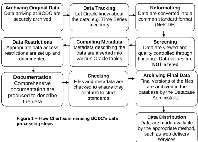
Moored instrument data go through several steps at BODC before they are incorporated in the National Oceanographic Database (NODB). Our aims are to ensure the data are of a consistent standard and to guarantee their long term security and utilisation. The data banking procedure involves reformatting of data files, quality control, entering information into Oracle tables, compiling documentation, and checking. All processes must be completed satisfactorily before the files can be archived in the database.

The NODB consists of a series of metadata inventories/tables which are held in an Oracle RDBMS (Relational Database Management System) and NetCDF data files which are held separately in a LINUX archive system. The data processing steps are outlined in the flow chart (Figure 1) and are explained more fully below.

3.2 Archiving Original Data

When data are received at BODC they go through an Accession Procedure. The data files are archived securely in their original form along with any associated documentation. Information describing the data is added to Oracle tables so we can keep track of all data obtained.

Data Tracking Let Oracle know about the data, e.g. Time Series

Inventory

Archiving Original Data

Data arriving at BODC are securely archived

Compiling Metadata

Metadata describing the data are inserted into various Oracle tables

Data Restrictions Appropriate data access restrictions are set up and

documented

Documentation

Comprehensive

documentation are

produced to describe

the data

Checking

Files and metadata are checked to ensure they

conform to strict standards

Reformatting

Data are converted into a common standard format

(NetCDF)

Archiving Final Data

Final versions of the files are archived in the database by the Database

Administrator

Screening

Data are viewed and quality controlled through flagging. Data values are

NOT altered

Figure 1 – Flow Chart summarising BODC‟s data processing steps

Data Distribution

Data are made available by the appropriate method,

such as web delivery services

(9)

BODC accepts data in most formats provided that the format is adequately described and that mandatory metadata are included. Most data are received in some kind of ASCII format, though some are received in binary formats such as MATLAB (.mat files). Data can be sent by various methods as mentioned in section 2.2

.

3.3 Data Tracking

Data tracking procedures ensure that the Oracle database system know about the data. Moored instrument time series data that are known to BODC are catalogued in the Time Series Inventory. This includes one row per instrument and is not restricted to data held at BODC. It can also include instruments which were lost or failed and also data which is held by other organisations. It currently contains over 13400 entries from 86 organisations and is available for searching online.

3.4 Parameter Dictionary

The BODC Parameter Dictionary is used for labelling data as they are submitted to BODC. Instead of using non-standard descriptions for parameters, individual codes are assigned from the dictionary. The code gives information about what was measured and can include additional information such as how the measurement was made.

During the 1990s BODC was heavily involved in the Joint Global Ocean Flux Study (JGOFS), which required rapid expansion of the dictionary to about 9000 parameters. When BODC first started managing oceanographic data in the 1980s, we dealt with less than twenty parameters. This rapid increase in the number of parameters forced us to adopt a new approach to parameter management and develop the dictionary. There are now dictionary entries for more than 18,000 physical, chemical, biological and geological parameters. Sometimes a single water bottle sample has been analysed for several hundred parameters. The dictionary is freely available and can be downloaded from:

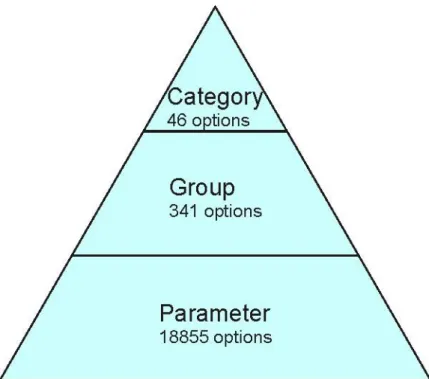
www.bodc.ac.uk/data/codes_and_formats/parameter_codes/bodc_para_dict.html Every Parameter is placed within a Group, linked by a 4-byte group code. To discover all Parameters within a particular Group, a search can be conducted using the group code. Groups are further classified into Categories to allow the user to focus a search starting at a very broad level. Examples of Categories are: acoustics, zooplankton, fatty acids. The top level of the hierarchy is the discipline (e.g. physics, chemistry, biology, etc.). Thus the hierarchy contains the following levels:

(10)

Figure 2: The data discovery hierarchy.

Each Category contains a subset of Groups. Each group contains a subset of Parameters. A user can focus a search for a Parameter or set of Parameters by navigating down the hierarchy.

3.5 Reformatting

As data arrive at BODC in various formats, the files need to be converted to a common standard format. It is important that all our data are held in one format as they can then be stored and distributed much more efficiently. It also ensures that parameter codes, flags, units, absent data values, etc. are consistent between files from different sources.

The format used for storing data at BODC is QXF (http://www.bodc.ac.uk/data/codes_and_formats/qxf_format/). QXF is based on the internationally recognised exchange format (NetCDF). It has the advantage of being able to handle multi-dimensional data from instruments such as moored Acoustic Doppler Current Profilers (ADCPs) and thermistor chains in one file. It is also platform independent and as it is array-based can be directly manipulated by MATLAB and other software packages. For further information on NetCDF, see http://my.unidata.ucar.edu/content/software/netcdf/index.html

.

MATLAB software, including the NetCDF and Database Toolboxes, is used for the reformatting of data. Although the main code relating the transfer procedure is generic, a new module is written to read in the data for each new format received. Therefore, it is very helpful if data are sent in a standardised format where possible as this makes the transfer procedure much more efficient. Eight-byte parameter codes from the BODC Data Dictionary are assigned to each data channel, data are converted to standard units and absent data values are set. If any quality control flags have already been applied by the data originator, these are kept in the QXF file.

(11)

Metadata (e.g. positions, depths) from file headers or additional files are also extracted to be loaded into Oracle tables later.

The transfer process is also the first line of quality control defence. Often problems or inconsistencies with the data/metadata are picked up at this stage as many checks are built in to the transfer software. Some automated data screening may also occur at this stage, such as the flagging of out-of-range values.

3.6 Screening

All data are manually screened at BODC by a data scientist using in-house visualisation software (Edserplo). This software can be used to display moored data as a time series. Current meter data are also be plotted as scatter plots and profiles can be plotted for ADCP (Acoustic Doppler Current Profiler) data.

Quality control is carried out through flagging. Parameters can be plotted concurrently and records from different instruments can be compared. Data values are NOT changed or removed, but may be flagged if they appear suspect. Data values that the originator regards as suspect are flagged with 'L'. BODC uses 'M' to flag suspect data. 'N' flag is used to indicate absent data. 'P' is used to indicate calm conditions (for e.g. wave height data), 'Q' is used to indicate indeterminate; for example for wave period data which cannot be satisfactorily determined during calm conditions.

3.7 Compiling Metadata

The metadata (information about the data), such as collection date and times, mooring position, instrument type, instrument depth and sea floor depth are loaded into Oracle relational database tables. These fields of the main ―series header‖ table for the National Oceanographic database are described in Annex 1. The values are carefully checked for errors and consistency with the data. The data originators may be contacted if any problems cannot be clearly resolved. Each data file has one row in the primary metadata table which is then linked to other tables that contain metadata relating more specifically to moorings, fixed stations, projects, cruises, etc.

3.8 Data Restrictions

Data may be restricted for a specified period or until a set date after the end of a project. It is important to ensure appropriate data access restrictions are set up to avoid data being supplied to a third party during the restricted period. Exceptions may be made for scientists working on the project or if authorisation has been given from the data originator to supply the data. All SIMORC data held in the BODC

(12)

ambiguity or uncertainty. The documentation is compiled using information supplied by the data originator (e.g. data reports, comments on data quality) and any further information gained by BODC during screening. It will include information such as mooring details, instrumentation, data quality, calibration and processing carried out by the data originator, and BODC processing and quality control. If any particular major problems are associated with the data, these can be described in a Problem Report. General comments are stored in Data Quality Reports.

A document management system is used to load and link the documents which are stored as tagged XHTML in Oracle tables.

A Series Metadata Report for each data file containing all of its linked documentation is available on the internet at http://www.bodc.ac.uk/data/documents/series/ishref/, using Web Services, where ishref is the data series reference number.

e.g.http://www.bodc.ac.uk/data/documents/series/702665/

3.10 Quality Checking

Before the data set can be loaded to the database, the QXF files and Oracle metadata are thoroughly checked to ensure they conform to stringent BODC standards. MATLAB software is used through a GUI interface to do this. Checks include:

 Channel limits are within the prescribed range for the parameter or are flagged if they are out with the range

 Time channel is increasing

 Null flags correspond with absent data values

 File doesn‘t begin or end with null data cycles

 Start and end time in data file and Oracle table agree

 No problems with QXF data file format

 Data series linkages

 Checks for gaps in data

Google Earth is also used to check positions. The screening and documentation are then also audited by a second person, as this can be helpful in highlighting any inconsistencies in flagging.

3.11 Archiving Final Data

Once the files have been screened and checked, the archiving of the final data set is performed by the BODC Database Administrator. The files are renamed and archived into the file system and the Oracle tables are updated to indicate the banked status of the data.

3.12 Data Distribution and Delivery

The data can then be distributed by a method appropriate for the project, such as through web delivery services or on CD ROM. If the user requires data in an

(13)

alternative format, the data can be translated into a specific ASCII formats or other NetCDF formats, such as WOCE NetCDF before supplying.

In the case of SIMORC, the data will not be available from BODC, as it will be made available by MARIS via the SIMORC website. Any enquirers requesting the data from BODC will be redirected to the website.

(14)

4.0 Current Meter Data - Quality Control

4.1 Checklist of Metadata Required for Processing/QC/Documentation

The checklist and example information below shows the information used by BODC to ensure that the data are adequately described.

Owner Details

Name of country responsible for data e.g. UK Name of organisation responsible for data e.g. POL

Project Name (if applicable) e.g. Coastal Observatory Data Type (e.g. current, wave, sea level, met) e.g. Current Meter

Mooring/Instrument Details Instrument category (e.g. current meter, wave recorder)

e.g. Paddle wheel current meter

Mooring/Rig Number e.g. 1234

Instrument model and manufacturer e.g. Aanderaa RCM7

Principle of measurement? e.g. Vector averaged currents Any instrument modifications? e.g. N/A

Additional notes on mooring structure (e.g. buoyancy measures, number of sensors)

e.g. In total 4 current meters on the mooring, subsurface buoyancy

Additional notes on performance of mooring (incl. condition on recovery, events which may have affected the data etc.)

e.g. weed found close to current meter, possible fouling of data

Latitude of mooring (degrees) e.g. 53.85° Longitude of mooring (degrees) e.g. -3.26°

Time zone e.g. GMT/UTC

Site Area and Name of Site e.g. Irish Sea, ABC site

Method of position fix e.g. GPS

Water column Depth (m) e.g. 352m

Sea Floor Depth Qualifier (e.g. echo sounder, GEBCO)

e.g. GEBCO Depth of meter or shallowest sensor (e.g. ADCP

bin)

e.g. 300m Depth of deepest sensor (can be same as above)

(m) – (Specific for ADCPs and thermistors) e.g. N/A Interval depth between successive bins (m) –

(Specific for ADCPs and thermistors)

e.g. 20m Series Depth Field Qualifier? (e.g. Sea floor

reference etc)

e.g. Mean Sea Level

Timing Details

Date and Time of Deployment (UTC) e.g. 25/08/04, 10:00 Date and Time of start of usable data (UTC) e.g. 25/08/04, 10:20 Date and Time of Recovery (UTC) e.g. 14/04/05, 16:30 Date and Time of end of usable data (UTC) e.g. 14/04/05, 16:10 Nominal time interval between successive data

cycles in series (seconds)

(15)

Type of sampling (e.g. instantaneous, averaged) Current direction – vector averaged Temperature – instantaneous

Parameter Details Parameters measured and any definitions where the parameter is not obvious (See 3.3. BODC Parameter Dictionary below)

e.g. Current speed (LCSAEL01), current direction (LCDAEL01), temperature (TEMPPR01), salinity (PSALPS01), pressure (PREXPR01)

Data Processing Details

Originator's Data Format e.g. ASCII, .mat

Description of calibrations

Description of any data processing that has occurred (manufacturers and in-house)

4.2 BODC Parameter Dictionary codes

To get a comprehensive list of our parameter codes and their definitions, you can go to our online parameter dictionary at:

http://www.bodc.ac.uk/data/codes_and_formats/parameter_codes/bodc_para_dict.html From here you can download the Parameter code list, the Parameter Group code list and the Units of Measurement code list, among others.

To aid your search we have included the most frequently used Parameter Group codes and Parameter codes for current meter data below:

Frequently Used Parameter Group Codes for Current Meter Data: Parameter Group

Code

Description

RFVL

Parameters expressing the velocity (including scalar speeds and directions) of water column horizontal movement, commonly termed currents

LRZA Vertical water movement parameters including non-directional speeds TEMP Temperature of the water column

PSAL Salinity of the water column

Frequently Used Parameter code for Current Meter Data: Parameter Code Description

(16)

shipborne acoustic doppler current profiler LCEWZZ01 Eastward current velocity in the water column

LCEWEL01 Eastward current velocity (Eulerian) in the water column by in-situ current meter

LCEWLA01 Eastward current velocity (Lagrangian) in the water column by tracked drifting buoy

LCEWAP01 Eastward current velocity (Eulerian) in the water column by moored acoustic doppler current meter

LCEWAS01 Eastward current velocity (Eulerian) in the water column by shipborne acoustic doppler current profiler

LCDAZZ01 Current direction in the water column

LCDAEL01 Current direction (Eulerian) in the water column by in-situ current meter and correction to true North

LCDAEL02 Current direction (Eulerian) in the water column by in-situ current meter and correction to true North

LCDALA01 Current direction (Lagrangian) in the water column by tracked drifting buoy

LCDAAP01 Current direction (Eulerian) in the water column by moored acoustic doppler current meter and correction to true North

LCDAAP02 Current direction (Eulerian) in the water column by moored acoustic doppler current meter and correction to true North

LCDAAS01 Current direction (Eulerian) in the water column by shipborne acoustic doppler current profiler and correction to true North

LCSAZZ01 Current speed in the water column

LCSAEL01 Current speed (Eulerian) in the water column by in-situ current meter LCSAEL02 Current speed (Eulerian) in the water column by in-situ current meter LCSALA01 Current speed (Lagrangian) in the water column by tracked drifting

buoy

LCSAAP01 Current speed (Eulerian) in the water column by moored acoustic doppler current meter

LCSAAP02 Current speed (Eulerian) in the water column by moored acoustic doppler current meter

LCSAAS01 Current speed (Eulerian) in the water column by shipborne acoustic doppler current profiler

RFVLDR01 Downstream current velocity in a river by direct reading current meter

4.2.1 Web Services

BODC‘s parameter vocabulary can be accessed using web services.

A web service is a collection of protocols and standards used for exchanging data between applications or systems. Software applications written in various programming languages and running on various platforms can use Web services to exchange data over the Internet, in a manner similar to inter-process communication on a single computer. This interoperability (e.g. between Java and Python, or Windows and Linux applications) is due to the use of open standards.

Further information is available from the BODC Web Services home page: http://www.bodc.ac.uk/products/web_services/

(17)

4.3 Glossary



Acoustic Doppler Current Profiler (ADCP) – A current meter which measures

current direction in 3 dimensions. As opposed to the average current meter, an ADCP can measure current speeds and direction at varying depths using a principle known as the Doppler Shift



Bin (ADCP) – A depth where an ADCP will measure current direction and speed using the Doppler Shift principle. An ADCP will measure current speeds and directions at a number of ‗bins‘ above or below it, which are placed at regular depth intervals. Data gathered at those ‗bins‘ furthest away from the instrument is generally of a poorer quality than that data collected at closer ‗bins‘



Channel – Generally represents measurements of a particular parameter (e.g.

temperature): the term channel is used in preference to parameter because there can be more than one measurement of a particular parameter within a datacycle



Current – Regular flow of a mass of water. The flow is generally consistent and is

dependent on the properties of the water mass



Mooring Knockdown – High speed currents can cause the mooring to ‗fall over‘.

This can be seen in the time series as an increase in pressure, a result of the sensor being pushed down to a deeper depth than it was positioned at



Mooring/Rig – deployment holding various oceanographic instruments including

current meters, ADCPs, thermistors, wave riders etc



Trawling – This is a result of a ship/boat catching the subsurface buoyancy of the

mooring carrying it from its mooring location



u, v components – breakdown of velocity – northerly travel and easterly travel



Velocity – 2 dimensional property of a moving object, incorporating the speed at

which it travels and the direction in which it is travelling

4.4 Screening Procedure

BODC‘s in-house software for quality controlling current meter data comprises a visualisation tool called SERPLO (SERies PLOtting), developed in response to the needs of BODC, whose mandate involved the rapid inspection and non-destructive editing of large volumes of data. SERPLO allows the user to select specific data sets and view them in various forms, to visually asses their quality. Displays include timeseries, depth series, a scatter plot for current meter data, an X-Y plot and a year‘s display for tidal data. There is also a world map covering the locations of series. Screening essentially allows the quality control of data that we receive with checks being made to ensure that the data are free from instrument-generated spikes, gaps, spurious data at the start and end of the record and other irregularities, for example long strings of constant values. These problems are not immediately obvious when just looking at large columns of data. When suspicious values are seen, flags are applied to the data points

(18)

4.4.1 Time Series

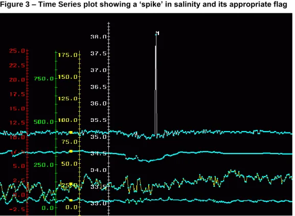
The most useful screening-view for current meter data is the time series; a plot of the parameters measured over the time of the record. This is useful as the user can get an idea very quickly about whether the data looks reasonable or not judging by the average values of the parameter measured and the overall ‗noisiness‘ of the plot. Using the time series all parameters can be visually ‗screened‘ with the aim of detecting anomalous values. Anomalous values are those which are out of character with the rest of the series and therefore unlikely to be a true representation. The most common are found as ‗spikes‘, usually caused by a problem with the instrument as opposed to a sudden rapid change in the water conditions. ‗Spikes‘ are usually singular points which are completely out-of-range when compared to the immediate surrounding values. It is possible that when there are a few data points within a single ‗spike‘ the values may represent a true event and as such these points making up the spike are not generally flagged unless they are hugely out of character with the rest of the series.

The figures below show examples:

Figure 3 – Time Series plot showing a „spike‟ in salinity and its appropriate flag

Figure 3 gives an example of a ‗spike‘ in salinity within a series. The spike has been flagged as suspect with the customary ‗M‘ flag. As can be seen only one point is out-of-range indicating it is likely to be an instrumental error.

(19)

Figure 4 – Time series plot showing „noisy‟ temperature, salinity and speed data

Figure 4 is an example of a situation where it is difficult to identify spikes because the surrounding data are noisy indicating a natural phenomenon having an effect on the localised water conditions.

It is helpful to screen related parameters, such as current speed and current direction together, to identify spurious values. It is common for related changes to occur with related parameters. If this is not seen it is often an indication that the event is not genuine and should be marked accordingly. For instance salinity is calculated from temperature. If there is a sudden change in salinity which is not seen in temperature it could just be due to a calculation error.

The derived velocity components can also be screened and indeed it is useful to check any suspect values in the speed or direction against the associated point in the u- and v-components.

(20)

Figure 5 - Example of a time series with a possible rotor problem

(Legend: Current Speed (ms-1), North velocity component (ms-1), East velocity component (ms-1), Current Direction (°), Temperature (°C) (not shown))

Figure 5 shows a typical time series plot of current speed and direction. In this specific example the current speeds are at the meter threshold level throughout the series, as can be seen by the period near the end of the plot where current speed and the velocity components ‗flatten out‘ to read near zero. This could mean that the rotor is being hindered in some way, therefore not turning freely and this should be noted in subsequent documentation.

Optical parameters such as transmittance can be compared with fluorescence or chlorophyll measurements. If there is an increase in chlorophyll levels for instance, you might expect to see a decrease in transmittance as light is blocked by the layer of chlorophyll. However, if this is not seen in the data the increase in chlorophyll may be a result of instrument error. However, in the same instance it may be the chlorophyll levels which are wrong and it is useful in these situations to check any accompanying documentation for additional information.

Where data series are noisy, perhaps a combined result of turbulent waters and the sensors not being able to adjust fast enough to changing conditions, it is harder to identify erroneous values. In cases like this only the extreme out-of-range data points are flagged, our policy being if unsure it is best not to flag the data point in question (see Figure 3).

Comparisons can be made between data from meters on the same rig by overlaying the time series plots on the workstation and by comparing the maximum and minimum

(21)

values of individual parameters. Similar comparisons are also made between data from neighbouring current meter moorings. Automatic checks are also made to ensure the time channel progresses forwards at equal intervals, problems have been encountered with time channels which jump backwards by a number of hours. In addition, the sampling interval is checked in conjunction with the number of data cycles in the series and the start/end time of the series. This is particularly useful when the time channel has not been supplied with the data (Rickards, 1989).

4.4.2 Data Limit Tests

Below are a range of tests taken from the IOC/CEC‘s ‗Manual of Quality Control Procedures for Validation of Oceanographic Data‘, 1993, which we can use to gauge whether the data is realistic or not:

a) Gross Error Limits i) Current Speed

Current speeds should not exceed the maximum speed which the current meter can measure based on the sampling period and scaling factor used, or 4ms-1, whichever is the smaller. The current speed should not be negative.

ii) Current Direction

All current directions should lie between 000º and 360º iii) Temperature

All temperatures should lie within the range of the sensor iv) Conductivity/Salinity

All conductivity values should lie within the range of the sensor

b) Rate of Range Checks i) Current speed and direction

Rate-of-change checks for current speed and direction are best applied to orthogonal components of the current velocity, since these can be considered to be cosine functions with definable expected differences between sampling points.

The theoretical differences between two consecutive current speed samples u1 and

u2 for various sampling intervals (∆t), assuming a smooth sinusoidal semi-diurnal

(22)

∆t (min) Theoretical |u1 – u2| Factor Allowable |u1 – u2| 5 0.0422 u 2.0 0.08ms-1 10 0.0843 u 1.8 0.15ms-1 15 0.1264 u 1.6 0.20ms-1 20 0.1685 u 1.5 0.25ms-1 30 0.2523 u 1.4 0.35ms-1 60 0.5001 u 1.2 0.60ms-1

:where u is the orthogonal tidal current amplitude. In order to allow for some inherent variability in current speed and direction signal and for asymmetric tidal current speed curves, these differences will have been increased by the above factors whilst u has been set at 1.0ms-1 since the variability will increase with decreasing u. The resulting allowable maximum difference between samples for particular sampling intervals is provided above.

ii) Sea Temperature |T1 – T2| ≤ ∆t

60

:where T1 and T2 are consecutive temperature measurements and ∆t is the sampling

interval in minutes.

iii) Conductivity/Salinity |S1 – S2| ≤ ∆t

60

:where S1 and S2 are consecutive salinity measurements and ∆t is the sampling

interval in minutes.

c) Stationarity Checks

The occurrence of constant values of data depends on the variable being measured, the sampling interval used and the resolution of the sensor.

i) Current Speed

Constant current speeds are uncommon although, theoretically, two consecutive values may be the same. A flag is set against each current speed which is equal in value to the two previous values, regardless of the sampling interval.

(23)

ii) Current Direction

Almost constant directions may be generated by topographic effects. The following numbers of consecutive equal values are allowed depending on sampling interval:

∆t (min) Number of Consecutive Equal Values 5 12 10 6 15 4 20 3 30 2 60 2

A flag should be set against each current direction point which is equal in value to the previous 12, 6, 4, 3 or 2 previous values (as applicable).

iii) Temperature

Constant temperature values are relatively common in well-mixed water, and the number of consecutive equal values allowed is thus large, being:

24 x 60 (i.e. up to one day is allowed) ∆t (min)

:where ∆t is the sampling interval in minutes. A flag should be set against all data points that are preceded by at least a day of constant values.

iv) Conductivity/Salinity

Constant salinity values are also relatively common in well-mixed water and a similar stationarity check to that for temperature is applied:

24 x 60 (i.e. up to one day is allowed) ∆t (min)

: where ∆t is the sampling interval in minutes. A flag should be set against all data points which are preceded by at least a day of constant values.

(24)

scatter plot allows you to find out more about the following: the extent and orientation of the current ellipse, the presence of outlying points and the relative size of the respective plots. They can be used in conjunction with the time series plot to check that outliers have been flagged.

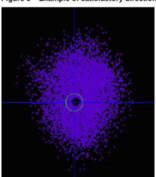
These plots can also show irregularities in the data, mainly as a result of mechanical malfunction. Examples of malfunctions show up as larger-than-anticipated holes, abnormal symmetry in the tidally-dominated regimes, gaps where a range of speeds or directions are not registered due to meter malfunction, or preferential directions where the compass was not functioning correctly. A typical scatter plot should show symmetry as tides often have regular patterns (e.g. diurnal) with regular speed minima and maxima and directions showing cycles of alternating opposing flow. The orientation and rotation of the tidal ellipse are compared for meters on the same rig and sometimes when possible with meters from neighbouring rigs.

Examples of scatter plots are shown below in Figures 6 and 7:

Figure 6 – Example of satisfactory directional data from a data series

Figure 6 shows an example of a ‗good‘ scatter plot. There seems to be an even array of current directions indicating that the compass was not being hindered.

However, Figure 7 below is an example of a record with suspect directions, as there are very few measurements from approximately 40° to 180°. This specific problem was attributed to the influence of the angle of the Earth‘s magnetic field on the compass of an Aanderaa RCM5 current meter.

(25)

Figure 7 – Example of unsatisfactory directional data from a data series

4.4.4 Common Problems Associated with Current Meters

There are a number of things that can go wrong with a deployed current meter which can affect the quality of the data. This is one of the main reasons why we visually screen data because instrumental errors can be picked up easily. Some of the more common instances when a meter has malfunctioned, resulting in a large loss of data, are:

 Rotor turns, but there is either a breakdown of magnetic coupling between the rotor and follower or reed switch which then fails to register rotations

 Rotor not turning due to fouling with weed or suchlike. This results in a sudden drop in speed to zero or near zero.

 Directions not being resolved. This could result from a stiff meter suspension or a meter being fouled by its mooring wire.

 Compass sticking. This may occur if the meter is inclined too far from the horizontal plane and can be a problem in fast tidal streams when in-line instruments are used. This is commonly known as ‗mooring-knockdown‘. This is

(26)

 Sticking encoder pins. These cause spikes in all parameters and are often manifested by the appearance of the value of the pin(s) in the listing (e.g. 0, 256, 512, 768 or 1023).

 Underrated power supply. This often shows in the compass channel first because of the extra current drain during clamping.

 Electronic failure (e.g. dry joints, circuitry broken). This does not always produce a total loss of data however.

 Poor quality recording tape. This is indicated by the appearance of suspect data at regular intervals in all parameters.

 Sensor drift. This is a slow change in the response of the sensor.

4.4.5 Differences in Screening Procedure for ADCPs and Thermistors

ADCPs and thermistor chains are different to current meters in that they sample in three dimensions. While ADCPs essentially measure the current in the horizontal plane, they are also able to measure the current at different depths, commonly known as bins, above or below the positioning of the instrument. This is done using the principle of the Doppler shift. An example of an ADCP profile is shown in Figure 8 below:

(27)

Thermistors chains are similar, but sample temperature at different bin levels. The screening procedure for these three dimensional data types is similar in principle to that for the normal current meter. The aim is to check for instrument-generated spikes, gaps, repetitive values, and spurious data types at the start and end of the series. Often, the data for one parameter will be observed on the screen at all its measured bin levels. This is useful to show up spikes which may occur up or down the water column. If a spike is present throughout the vertical it may be a valid point due to actual changes in the water properties. However if it is a one-off point in a single bin then the likelihood of it being valid is reduced.

4.6 Accompanying Documentation

At BODC we include a set of standard documentation with every data series. Using in-house software this documentation is ‗linked‘ to the data series in Oracle and when data is requested the accompanying documentation is provided. Example documentation can be found in Annex 2. The most common documents written for each dataset are as follows:

 Data Activity – this document describes the ‗event‘. In the case of current meters it generally gives the dates of deployment, description of the location of the mooring and its setup, including the latitude and longitude, and the depths and meter numbers of all the other sensors present on the mooring. Any other information to the event is included in this document. This document is linked to every data series which has been collected from the same mooring.

 Data Quality Document – this document is linked to individual series and is not generic. Any comments or problems relating to the data series are included in this document as well as any steps taken to resolve the problem. Often this is provided by the data originator, where they have taken steps to improve the quality of the data, and our input is generally made up of comments from the screening process.

 Project Report – This is a document describing the project for which data is collected. This is a generic document which is linked to every data series involved with a particular project.

 Fixed Station Document – This gives information on a particular station which is used consistently for measurements over time.

(28)

 Instrument Document – This is a generic document linked to every series which has been produced from a particular instrument. The document includes information on how the instrument works, its sensitivity, accuracy and links to the manufacturer‘s website where applicable.

(29)

5.0 Wave Data - Quality Control

Owner Details

Project Name (if applicable) e.g. Coastal Observatory Data Type (e.g. current, wave, sea level, met) e.g. Wave Statistics

Mooring/Instrument Details

Instrument category (e.g. current meter, wave recorder)

e.g. Wave recorder

Instrument model and manufacturer e.g. Datawell Waverider Principle of measurement? e.g. Accelerometer Any instrument modifications? e.g. N/A

Additional notes deployment e.g. Any known data gaps / dropout problems

Additional notes on performance of mooring e.g. high-frequency cut-off Latitude of mooring (degrees) e.g. 53.85°

Longitude of mooring (degrees) e.g. -3.26°

bin)

e.g. 300m

Timing Details

Date and Time of Deployment (UTC) e.g. 25/08/04, 10:00 Date and Time of start of usable data (UTC) e.g. 25/08/04, 10:20 Date and Time of Recovery (UTC) e.g. 14/04/05, 16:30 Date and Time of end of usable data (UTC) e.g. 14/04/05, 16:10 Nominal time interval between successive data

cycles in series (seconds)

(30)

Frequently Used Parameter Group Codes for Wave Data: Parameter Group

Code

Description

GTDH Parameters expressing the significant wave height GTZA Zero upcrossing period

GCMX Maximum recorded wave height GTPK Spectral peak wave period.

Frequently Used Parameter Codes for Wave Data:

Code Description

GPEDFA01

Spectrum peak energy direction of waves on the water column by waverider and Fourier analysis

GPSPFA01

Directional spreading at spectral peak of waves on the water column by waverider and Fourier analysis

GSPKFA01

Spectral peakedness factor of waves on the water column by waverider and Fourier analysis after Goda (1970)

GSWDFA01

Spectral width of waves on the water column by waverider and computation from moments as defined by Cartwright and Longuet-Higgins (1956)

GTPKFA01

Spectral maximum period of waves on the water column by waverider and Fourier analysis

GAVGEV01 Average height of waves on the water column by visual estimation GAVGVA01 Average height of waves on the water column by waverider GAVHCA01

Average height of waves (highest 1/3rd) on the water column by waverider and automated record analysis

GAVHCS01

Average height of waves (highest 1/3rd) on the water column by wavestaff and automated record analysis

(31)

GAVHMA01

Average height of waves (highest 1/3rd) on the water column by waverider and manual record analysis

GCARFA01

Characteristic height of waves {Hrms*4} on the water column by waverider and Fourier analysis

GCARMA01

Characteristic height of waves {Hrms*4} on the water column by waverider and manual record analysis

GCMXCA01

Maximum height of waves on the water column by waverider and automated record analysis

GCMXVA01 Maximum height of waves on the water column by waverider GHSWEV01 Height of swell waves on the water column by visual estimation GMNLCA01

Minimum level of waves on the water column by waverider and automated record analysis

GMX1CA01

Maximum height of waves (in 1-hour period) on the water column by waverider and automated record analysis

GMXACA01

Maximum level plus minimum level of waves on the water column by waverider and automated record analysis

GMXHCA01

Maximum height of waves (in 3-hour period) on the water column by waverider and automated record analysis

GMXHFA01

Maximum height of waves (in 3-hour period) on the water column by waverider and Fourier analysis

GMXHMA01

Maximum height of waves (in 3-hour period) on the water column by waverider and manual record analysis

GMXHTD01

Maximum height of waves (in 3-hour period) on the water column by water level recorder pressure sensor

GMXLCA01

Maximum level of waves on the water column by waverider and automated record analysis

GPSWEV01 Swell period of waves on the water column by visual estimation GRMSCA01

Root mean square displacement of waves on the water column by waverider and automated record analysis

GRMSVA01

Root mean square displacement of waves on the water column by waverider

GTCACA01

Average crest period of waves on the water column by waverider and automated record analysis

GTCACP01

Average crest period of waves on the water column by water level recorder pressure sensor and automated record analysis

GTCAEV01

Average crest period of waves on the water column by visual estimation

GTCAZZ01 Average crest period of waves on the water column GTDHCA01

Significant height of waves {Hs} on the water column by waverider and automated record analysis

GTDHCS01

Significant height of waves {Hs} on the water column by wavestaff and automated record analysis

(32)

attenuation correction

GTDHVA01 Significant height of waves {Hs} on the water column by waverider GTDHZZ01 Significant height of waves {Hs} on the water column

GTKCMA01

Second maximum level of waves on the water column by waverider and manual record analysis

GTKCMP01

Second maximum level of waves on the water column by water level recorder pressure sensor and manual record analysis

GTKDMA01

Second minimum level of waves on the water column by waverider and manual record analysis

GTKDMP01

Second minimum level of waves on the water column by water level recorder pressure sensor and manual record analysis

GTZACA01

Average zero crossing period of waves {Tz} on the water column by waverider and automated record analysis

GTZACP01

Average zero crossing period of waves {Tz} on the water column by water level recorder pressure sensor and automated record analysis GTZACS01

Average zero crossing period of waves {Tz} on the water column by wavestaff and automated record analysis

GTZAFA01

Average zero crossing period of waves {Tz} on the water column by waverider and Fourier analysis

GTZAFB01

Average zero crossing period of waves {Tz} on the water column by shipborne wave recorder and Fourier analysis

GTZAFP01

Average zero crossing period of waves {Tz} on the water column by water level recorder pressure sensor and Fourier analysis

GTZATD01

Average zero crossing period of waves {Tz} on the water column by pressure sensor

GTZAUP01

Average zero crossing period of waves {Tz} on the water column by water level recorder pressure sensor and Fourier analysis with NO depth attenuation correction

GTZAVA01

Average zero crossing period of waves {Tz} on the water column by waverider

GTZAZZ01 Average zero crossing period of waves {Tz} on the water column GTZHCA01

Average zero crossing period (highest one third) of waves on the water column by waverider and automated record analysis

GTZHCS01

Average zero crossing period (highest one third) of waves on the water column by wavestaff and automated record analysis

GTZMCA01

Maximum zero crossing period of waves on the water column by waverider and automated record analysis

GTZMCS01

Maximum zero crossing period of waves on the water column by wavestaff and automated record analysis

GZMXCA01

Maximum zero crossing height of waves on the water column by waverider and automated record analysis

GZMXCS01

Maximum zero crossing height of waves on the water column by wavestaff and automated record analysis

GZMXFA01

Maximum zero crossing height of waves on the water column by waverider and Fourier analysis

GDSWEV01 Direction of swell waves on the water column by visual estimation GDSWZZ01 Direction of swell waves on the water column

GSPRFA01

Directional spread of waves on the water column by waverider and computation from cross spectra

(33)

GWDRZZ01 Direction of waves on the water column

5.2.1 Web Services

BODC‘s parameter vocabulary can be accessed using web services.

A web service is a collection of protocols and standards used for exchanging data between applications or systems. Software applications written in various programming languages and running on various platforms can use Web services to exchange data over the Internet, in a manner similar to inter-process communication on a single computer. This interoperability (e.g. between Java and Python, or Windows and Linux applications) is due to the use of open standards.

Further information is available from the BODC Web Services home page: http://www.bodc.ac.uk/products/web_services/

(34)

5.3 Glossary

 Hs : Significant wave height - measure of the average height of the highest one third of waves during the record in metres

 Tz: Zero upcrossing period - the mean wave period (taken as the average time between consecutive crossings of the mean sea level line in an upwards direction) in seconds

 Tmax: Maximum wave height - maximum recorded wave height in metres  Tcrest: Crest period - time taken between consecutive crossings of wave crests  Tpeak: Peak period also known as dominant wave period - it is the period corresponding to the frequency band with the maximum value of spectral density

5.4 Screening and QC Procedures – All Wave Data

After reformatting using BODC‘s in house Transfer system, data will be screened on a graphics workstation. BODC‘s in-house software for quality controlling current meter data comprises a visualisation tool called SERPLO, developed in response to the needs of BODC whose requirement involved the rapid inspection and non-destructive editing of large volumes of data. SERPLO allows the user to select specific data sets and to view them in various forms, to visually asses their quality. Screening essentially allows the quality control of data that we receive with checks being made to ensure that the data are free from instrument-generated spikes, gaps, spurious data at the start and end of the record and other irregularities, for example long strings of constant values. These problems might not otherwise be picked up if just viewing large columns of figures. When suspicious values are seen, flags are applied to the data points in question as a warning to end users. BODC uses two types of flag, M and N. The M flag is assigned to suspicious values, whereas the N flag is assigned to those values that are null. These flags do not change the data; they purely highlight potential problems with the data, allowing the end user to make the decision as to whether to use the data or not. 'P' is used to indicate calm conditions (for e.g. wave height data), 'Q' is used to indicate indeterminate; for example for wave period data which cannot be satisfactorily determined during calm conditions

5.4.1 Time Series Plots

Using the time series plot all parameters can be visually ‗screened‘ with the aim of looking for anomalous values. Often, related parameters, such as significant wave height and maximum wave height, are screened together to identify spurious values. This is because if there is a sudden change in one of the parameters you might expect to see a change in the other in agreement that it is a genuine event.

(35)

Figure 9 – Time Series of Zero Upcrossing Period and Significant Wave Height

The time series plot shown in this example is that of zero upcrossing period shown in red and significant wave height shown in green.

The time series plots will be used to identify:

 Instrument failure test (10 or more consecutive points of identical value)

 Wandering mean test (interval between successive upcrossings of >25 seconds)  Check that Tz falls within the range 2-16 seconds

 Check that Tpeak falls within the range 3 -20 seconds  Check that Tz not less than Tcrest

(36)

 Check for stationarity: assuming that the wave field is not rapidly evolving or decaying, records of wave height and period should be broadly similar from one record to the next

5.4.2 Scatter Plots

Another useful tool provided by SERPLO is the ability to produce scatter plots of wave height against (zero upcrossing or crest) period, as shown below:

Figure 10 – Scatter plot of wave height against period

These plots can show unrealistically steep waves with a slope of more than 1:10. They can also show outliers from the cluster of Tz vs. Hs values. Similarly, wind speed versus wave height scatter plots can be used to identify outliers from the clusters (NB make allowances for swell waves, which will show higher than expected wave heights for a given wind speed).

Checks will be made for:

 Definition of unacceptable steepness and appropriate flagging (ratio of Hs/Tz)  Outliers of clusters of Ts/Hz and of Ts versus wind speed

(37)

5.4.3 Frequency Plots

A useful tool provided by SERPLO is the ability to produce frequency distributions of significant wave heights. The tail ends of the distributions can be analysed to identify where instrument noise becomes detectable, and a threshold or filter set accordingly.

5.4.4 QC Procedures – 1D and Directional Wave Spectra

 Check slope of energy density spectrum – should follow a set slope due to transfer of energy from lower to higher frequencies

 Check that energy in the spectrum at frequencies below 0.04 Hz is not more than 5% of the total spectral energy

 Check that energy in the spectrum at frequencies above 0.6 Hz is not more than 5% of the total spectral energy

 Check mean direction at high frequencies, which should correspond to the wind direction (assuming coincident meteorological data.

 For 1D spectra, calculate zeroth spectral moment from spectral variance densities and check that it corresponds to the given value

 For 1D spectra, calculate Te as the zeroth divided by first negative spectral moment and check that it correlates with (peak or zero upcrossing) period

5.5 Problems Associated with Wave Data

The main problems are expected to be constant values and possibly wandering means, which will be identified as above.

5.6 Accompanying Documentation

At BODC we include a set of standard documentation with every data series. Using in-house software this documentation is ‗linked‘ to the data series in Oracle and when data is requested the accompanying documentation is provided. Example documentation can be found in Annex 2. The most common documents written for each dataset are as follows:

 Data Activity – this document describes the ‗event‘. In the case of wave buoys or similar it generally gives the dates of deployment and description of the location including the latitude and longitude. Any other information to the event is included in this document. This document is linked to every data series that has been collected from the same mooring.

(38)

 Project Report – This is a document describing the project for which data is collected. This is a generic document which is linked to every data series involved with a particular project.

 Fixed Station Document – This gives information on a particular station that is used consistently for measurements.

 Restrictions Document – This document outlines any restrictions imposed on particular datasets and who the main contact is for any questions relating to the data.

 BODC Screening Document – This is a generic document linked to all datasets giving a brief summary of the screening procedure BODC undertakes for each dataset, so the external user is aware of the broader quality control that takes place.

 Instrument Document – This is a generic document linked to every series which has been produced from a particular instrument. The document includes information on how the instrument works, its sensitivity, accuracy and links to the manufacturer‘s website where applicable.

(39)

6.0 Sea Level Data – Quality Control

Owner Details

Project Name (if applicable) e.g. Coastal Observatory Data Type (e.g. current, wave, sea level, met) e.g. pressure/water level

Mooring/Instrument Details

Instrument category (e.g. current meter, wave recorder)

e.g. Water Level Recorder

Instrument model and manufacturer e.g. Aanderaa WLR Principle of measurement? e.g. pressure sensor Any instrument modifications? e.g. N/A

Additional notes deployment e.g. Any known data gaps / dropout problems

Additional notes on performance of mooring e.g. high-frequency cut-off Latitude of mooring (degrees) e.g. 53.85°

Longitude of mooring (degrees) e.g. -3.26°

bin)

e.g. 300m Depth of deepest sensor (can be same as

above) (m) – (Specific for ADCPs and thermistors)

e.g. N/A

Interval depth between successive bins (m) –

(Specific for ADCPs and thermistors)

e.g. 20m Series Depth Field Qualifier? (e.g. Sea floor

reference etc)

(40)

Type of sampling (e.g. instantaneous, averaged)

Parameter Details

Parameters measured and any definitions where the parameter is not obvious (See 6.2. BODC Parameter Dictionary below)

e.g, pressure (PREXPR01)

Data Processing Details

Frequently Used Parameter Group Codes for Sea Level Data: Parameter Group

Code

Description

AHGT All vertical spatial parameters including depth, height and pressure when used as an independent variable.

ASLV Measurements and predictions of the displacement of the water column surface from a fixed, stable reference

CAPH

Measurements of air pressure as the dependent variable (ie excluding air pressure measured to specify the z co-ordinate of a balloon or sonde), including derived parameters such as tendency (rate of change) and related parameters such as air density.

PREX

Measurements of the displacement of the water column surface from a fixed, stable reference expressed as either total pressure or sea pressure