method was used, and the adsorption isotherm of CH4on snow at 77 K was recorded. The
data were analyzed by the Brunauer-Emmett-Teller method to yield SSA andQCH4, the
mean heat of adsorption of the first CH4 monolayer. SSA values obtained were between
100 and 1580 cm2/g. The reproducibility of the method is estimated at 6%, and the accuracy is estimated at 12%. We propose thatQCH4= 2240 ± 200 J/mol should be used
as a criterion of reliability of the measurement. The method is described in detail to promote its use. Aged snow samples have lower SSA than fresh ones. The lowest values were found for faceted crystals and depth hoar, and the highest values were found for fresh rimed dendritic snow. A method that field investigators can use to estimate SSA from a visual examination of the snow and from a density measurement is suggested. Snow samples are classified into 14 types based on snow age and crystal shapes. Within each type, a density versus SSA correlation is determined. Our data indicate that, depending on snow type, SSA can then be estimated within 25 to 40% at the 1sconfidence level with the method proposed. Preliminary data suggest that SSA spatial variability of a given snow layer is low (<5%), but metamorphism can increase it. INDEXTERMS:1863 Hydrology: Snow and ice (1827); 3947 Mineral Physics: Surfaces and interfaces; 0399 Atmospheric Composition and Structure: General or miscellaneous; 0320 Atmospheric Composition and Structure: Cloud physics and chemistry;KEYWORDS:surface area, snow, adsorption, chemistry, air-snow exchange
Citation: Legagneux, L., A. Carbanes, and F. Domine´, Measurement of the specific surface area of 176 snow samples using methane adsorption at 77 K,J. Geophys. Res.,107(D17), 4335, doi:10.1029/2001JD001016, 2002.
1. Introduction
[2] Some aspects of atmospheric chemistry above snow-covered surfaces are not well understood. Among these aspects is springtime ozone depletion [Barrie et al., 1988]. Despite years of investigation, modeling this complex chemistry remains uncertain, and the actual role of the snowpack still has to be elucidated [Michalowski et al., 2000]. Recently, the interest in studying the impact of the snowpack on the chemical composition of the lower tropo-sphere has increased, because new observations have shown that significant exchanges of reactive trace gases were taking place between the snow and the overlying air. Formaldehyde has been observed to come out of the snowpack in Greenland and in the Canadian high Arctic [Hutterli et al., 1999;Sumner and Shepson, 1999]. Fluxes of acetaldehyde and acetone coming out of the seasonal snow cover in Michigan were measured by Couch et al.
[2000]. Various nitrogen oxides were also observed to be exchanged between the snow and the atmosphere in Green-land and Antarctica [Dibb et al., 1998;Honrath et al., 1999;
Weller et al., 1999]. Ozone was found to be destroyed in
snow [Peterson and Honrath, 2000]. Snow chamber experi-ments, where air of controlled composition was passed through snow, confirmed that emission of carbonyls and nitrogen oxides by snow was taking place [Couch et al., 2000;Honrath et al., 2000].
[3] Thus because snow can cover up to 50% of landmasses in the Northern Hemisphere [Robinson et al., 1993;Frei and Robinson, 1998], the impact that this ground cover may have on the chemical composition of the lower troposphere is potentially very important on a global scale. The main reason why an accurate and reliable model of atmospheric chemistry in the presence of a snow cover does not exist is because the processes involved are not understood [Michalowski et al., 2000]. These processes include adsorption/desorption from the snow surface, which have been invoked to explain formaldehyde emission [Hutterli et al., 1999], photolysis of a dissolved precursor that has been postulated as the source of NOx coming out of the snow [Honrath et al., 1999;Weller et al., 1999] and which has been confirmed by laboratory experiments [Honrath et al., 2000], cocondensa-tion of trace gases with water vapor, with subsequent sub-limation of the solid solution formed [Weller et al., 1999], and solid state diffusion in and out of ice crystals [Domine´ and Thibert, 1996;Thibert and Domine´, 1998].
Copyright 2002 by the American Geophysical Union. 0148-0227/02/2001JD001016$09.00
[4] Determining which process is predominant requires the quantification of each one of them, which will neces-sitate many careful studies. The purpose of this study is to help quantify adsorption/desorption processes and the rates of heterogeneous reactions by reporting data that will aid in evaluating the surface area (SA) of a given volume of snow. By surface area we mean, followingGregg and Sing
[1982], the area of snow that is accessible to gases, and this area is expressed in square meters (or square centi-meters for small values). The SA of snow is evaluated from the measurement of the specific surface area (SSA) of snow samples, i.e., the SA of the sample divided by its mass, and this is expressed in square meters per gram (or rather in square centimeters per gram, as values of SSA for snow have been found to be small). The product of the density, SSA, and volume of the snow under consideration yields the SA of the snow. Values of snow SA, together with the knowledge of the adsorption isotherms of the atmospheric trace gas of interest on ice, can be used to quantify the amounts of trace gases adsorbed on ice and the rates of heterogeneous reactions.
[5] The method used here to measure snow SSA is CH4 adsorption at 77 K. The principle and merits of this method have been briefly described in previous publications [Hanot and Domine´, 1999; Domine´ et al., 2000, 2001], and we believe that it can yield reliable and reproducible results and that it is perhaps one of the fastest methods to obtain SSA values. Although the principle of the method is simple, performing reliable measurements is delicate, and we wish to report here a detailed protocol, propose selected values of parameters that could a priori be chosen somewhat arbitrarily in data analysis, suggest reliability tests, and mention com-monly encountered artifacts, so that other authors can use this method to obtain results that can be intercompared with ours. [6] Another objective of this work is to report the results of 176 snow SSA measurements, performed in the Alps and in the Arctic, and to attempt to find a correlation between snow types and SSA values, so that the values reported here can be used to estimate the SA of snow encountered in field studies.
2. Experimental Methods 2.1. Principle of the Method
[7] To determine snow SSA, the adsorption isotherm of CH4 on the snow sample is measured at liquid nitrogen temperature (77.15 K at atmospheric pressure), using a volumetric method [Gregg and Sing, 1982]. The isotherm is then analyzed by using a Brunauer-Emmett-Teller (BET) method [Brunauer et al., 1938] to obtain the SA of the sample and the net heat of adsorption of CH4 on ice, QCH4.
[8] Most SA measurements using the volumetric method have dealt with materials of high SSA and used N2as the adsorbent [Gregg and Sing, 1982]. The use of a commercial apparatus designed for high SSA materials to measure snow SSA, has been attempted byHoff et al.[1998], but as was mentioned by Hanot and Domine´ [1999], numerous arti-facts were encountered in that study, resulting in large errors. Because snow samples used here had a SA of only about 1 m2, modifications had to be made to the conven-tional volumetric apparatus. The apparatus used and the protocol followed have been briefly described by Chaix
et al. [1996] and Hanot and Domine´ [1999] and will be discussed in more detail here.
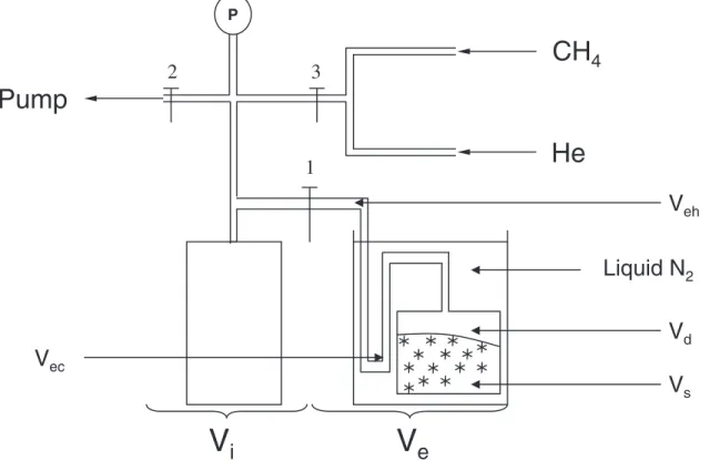
[9] The apparatus is shown in Figure 1. It consists of an introduction volumeVi kept at room temperature and
con-nected to a capacitance manometer (MKS Baratron, 10-torr full scale) and to an expansion volumeVethat contains the
snow sample and is immersed in liquid N2.
[10] The adsorption isotherm is recorded as follows. A given pressure of CH4,P10, is introduced intoVi. Knowing
Vi and P10, the number of molecules of CH4 in Vi, N10, is calculated by using the ideal gas equation. The valve betweenViandVeis then opened. The CH4pressure drops owing to expansion and adsorption. The new pressure,P001, is used to calculateN001, the number of CH4molecules still in the gas phase. The number of adsorbed molecules after this first CH4 increment is then Nads1 = N10 N001. Further increments are added, and the total number of molecules adsorbed after the addition ofnincrements of CH4is
Nntads¼ Vi RTh X n 1 P0kP 00 k P 00 n R Veh Th þVd Tc ! A; ð1Þ
where R, A, Th, and Tc, are the ideal gas constant, the
Avogadro number, and the ambient and liquid nitrogen temperatures, respectively.Vehis the part of the expansion
volume that is at room temperature, and Vd is the dead
volume (see Figure 1 for details). Pk0 and Pk00 are the
pressures before and after expansion of gas incrementk. [11] The adsorption isotherm can then be plotted, and an example is shown in Figure 2. The adsorption isotherm is of type II in the classification ofBrunauer et al.[1940] and lends itself to the BET treatment [Brunauer et al., 1938]. Briefly, a function Y = f(PCH4/P0) is plotted, where P0 is the saturating vapor pressure of CH4 at liquid nitrogen temperature. The plot of Y yields a linear portion, whose slopeSand interceptIyield the monolayer capacity of the sample, Nm = 1/(S + I), and the so-called BET constant,
C = (S + I)/I. The SA of the sample is then deduced as SA =Nmsm, wheresm= 19.1810
20
m2[Chaix et al., 1996] is the molecular cross-sectional surface area of CH4 on ice. The net heat of adsorption of CH4on snow,QCH4, i.e., the mean heat of adsorption of the first CH4 mono-layer, can also be derived from QCH4 = RT ln (C), whereRis the gas constant. The mass of the snow sample is then determined by weighing, and the SSA is obtained as the ratio of SA over mass. The BET transform of the isotherm of Figure 2 is shown in Figure 3. The linear part is roughly in the relative pressure P/P0region 0.07 to 0.22. 2.2. Apparatus and Data Treatment Optimization
[12] Measuring small SA values required changes to the standard volumetric equipment. First of all, CH4was used as the adsorbent rather than N2for five main reasons: (1) its low saturating vapor pressure, P0= 1294 Pa, justifies the use of the ideal gas equation without any correction; (2) low pressures minimize the amount of CH4 used, which is an advantage for field campaigns in remote areas; (3) the low
P0means that smaller amounts of CH4than N2need to be introduced intoVe, thus reducing the risk of snow annealing
relative pressure changes will be greater than those for N2, which will improve the accuracy of the measurements, and this aspect was found to be crucial to obtain quality measurements; and (5) methane is a spherical molecule that has neither a dipole nor a quadrupole moment, in agreement with the approximations of the BET theory [Brunauer et al., 1938].
[13] Another important aspect is the ratio Vi/Ve, which must be chosen adequately to optimize data quality. Two opposite effects come into play to determine the optimum ratio: (1) ifViis too high, expanding the gas fromVitoVe
will not change the pressure enough to produce a detectable effect on the manometer; this loss of sensitivity will also increase the impact of the manometer thermal drift in that a
Figure 1. Experimental setup. The introduction volumeViis delimited by valves 1 to 3 and is at room
temperature. The expansion volume Veconsists of Veh at ambient temperature andVec at 77 K.Vec is
subdivided into the snow volumeVs and the dead volumeVd. P is the manometer.
Figure 2. Example of an adsorption isotherm of CH4on snow. The number of molecules adsorbed per gram of snow,Nntads, is plotted as a function of the reduced CH4pressure,P/P0, whereP0is the saturating vapor pressure at liquid nitrogen temperature.
drift of one unit will represent a larger proportion of the pressure change, which will decrease data reliability; and (2) ifViis instead too small, reaching the pressure required
to use the BET treatment would necessitate more incre-ments; since errors caused by each increment add up, a smallViwill increase the uncertainty.
[14] Determining the optimum ratio by considering equa-tions is not simple. Moreover, the optimum is different for each snow sample, as what actually comes into play is notVe,
but the dead volume Vd = Ve Vs, where Vs is the snow
volume, andVdvaries with each snow sample. The expansion
ratioP0/P00during adsorption also comes into play and varies with each snow sample as it depends on sample SA. Empiri-cally, we observed that usingVi/Vebetween 0.5 and 2 gave
good quality data. The apparatus used to obtain most of the data presented here usedVi= 287.3 cm3andVe= 263.3 cm3,
and the volumes were connected by a tubing with a 4-mm inner diameter, which is sufficiently large to avoid thermal transpiration problems, as detailed in the next section.
[15] The use of the BET treatment requires the selection of a linearP/P0range in the BET transform (Figure 3). This selection and the number of data points obtained in this portion of the isotherm are somewhat arbitrary. Both SA and QCH4 were slightly affected by the selection of the linear range. It is essential to propose a range that is common to all experimentalists to facilitate intercompari-sons and to allow a test of the reliability of the measure-ments. Moreover, Domine´ et al. [2000] proposed that the value ofQCH4could be used to test the reliability of SA measurements. If this test is to be reliable, then arbitrary choices that cause variations inQCH4must be minimized. [16] By searching the optimum correlation coefficient of the least squares fit of the BET transform, it appeared that the best range for P/P0 was 0.07 to 0.22. The number of
data points within this range is also important. It has to be sufficient to obtain a reliable fit, but since errors add up at each data point, there is also an optimum number. Using nine data points within thisP/P0range was found to be a good compromise, and we recommend using this number. Under those conditions, 176 measurements done by two different experimentalists yieldedQCH4±s= 2240 ± 100 J/mol. We then recommendQCH4±s= 2240 ± 200 J/mol as a test of measurement reliability. Shifting theP/P0range by 0.02 induced about 3% changes inQand 2% changes in SSA.Domine´ et al.[2000], on the basis of a limited data set, had temporarily proposedQCH4= 2100 ± 150 J/mol. The new recommendation is consistent with the previous one but is based on a much larger data set.
2.3. Common Artifacts and Sources of Errors
[17] Artifacts and large sources of error can be encoun-tered at several stages of SSA measurements with the present method. These include the formation of amorphous ice of very high surface area during sample cooling, snow annealing by rapid injection of warm gas, perturbation of the snow during sampling, errors in temperature measure-ments or temperature instabilities, errors in pressure meas-urements, and errors in the determination of the dead volume above the snow. These are detailed below.
[18] Amorphous ice formed at 77 K is microporous and can have a SSA of several hundred square meters per gram [Mayer and Pletzer, 1987]. Because our snow samples had SA of around 1 m2, even the formation of a small fraction of a gram of amorphous ice can considerably increase the SA of the sample. SSA values found were between 100 and 1580 cm2/g. Values above about 5000 cm2/g should in general be considered suspect, and a desorption isotherm should then be measured to check for the presence of porosity. For example,
Figure 3. BET transform of the isotherm of Figure 2. A linear portion can be seen. The least squares fit in theP/P0region 0.07 to 0.22 is shown and has been used to obtain the snow sample SA and QCH4. The ordinateYis the BET transform (see text).
the snow used to obtain the hysteresis loop of Figure 4 was aged hard wind-packed snow, with an expected SSA of around 200 cm2/g. The SSA found was 20,800 cm2/g, which led us to measure desorption. An examination of the snow under a microscope is another method to check the validity of a very high SSA [Domine´ et al., 2001].
[19] Microporous ice could be formed by the condensa-tion of the water vapor in equilibrium with the snow in the container. However, simple calculations show that the amount of water vapor present in the expansion volume is much too small to yield detectable amounts of microporous ice. On the contrary, when the container with the snow sample is immersed in liquid nitrogen, large temperature gradients are established, which produce water vapor gra-dients and fluxes. To avoid amorphous ice formation, water vapor fluxes must be limited [Kouchi et al., 1994], and the snow sample must be cooled under a total pressure of about one atmosphere. The water vapor flux is proportional to the diffusion coefficient of water vapor in the gas filling the container, and this is inversely proportional to the total pressure. Keeping the snow under atmospheric pressure during cooling was found to be sufficient to prevent the formation of detectable amounts of microporous ice. The fact that optical and electron microscopy images of the snow yielded reasonable estimates of the SSA measured by CH4adsorption [Domine´ et al., 2001] also supports the fact that microporous ice formation can indeed be prevented by following this simple protocol.
[20] In our system, Viis at room temperature rather than at 77 K to minimize liquid N2 consumption during field experiments. Repeated injections of warm gas during adsorption measurements could anneal the snow and reduce its SSA. This was avoided by inserting a U-shaped tubing, which was immersed in liquid N2, betweenVi andVe(see
Figure 1). The efficiency of this procedure was checked by
measuring several consecutive isotherms and observing no changes in SSA.
[21] Sampling can perturb snow. Appropriate sampling must preserve the snow structure. That means, in particular, avoid breaking fresh snow crystals, avoid creating new contacts between snow grains by packing, and avoid creat-ing new surfaces by loosencreat-ing up sintered grains. For example, hard dense snow has to be broken into pieces to be inserted into the container. The maximum impact of breaking up hard snow on its SSA was measured. A very hard wind-packed snow layer with a density of 0.48, near the surface of the Arctic snowpack, was used. The snow was sampled in two ways: (1) the container was filled by loosening up grains from the vertical face of a pit dug in this snow layer; and (2) large chunks of at least 2 cm3 were broken up and inserted into the container; any small grains that may have inadvertently been placed in the container were removed by placing the container upside down. The first sampling method yielded a SSA of 312 cm2/g, while the second one yielded 147 cm2/g, showing that great care must be taken while sampling. No tests have been per-formed to evaluate the effect of packing fresh snow into a container on its SSA, but we checked on several occasions that density increases of fresh snow due to careful sampling were less than 10%, and we then suggest that careful sampling of fresh snow can minimize the creation of extra contacts between snow crystals.
[22] Drifts in the manometer gain can cause a systematic error in the pressure measurement. An ambient temperature different from that at which the manometer was calibrated can cause such drifts. We tested the effect of a systematic pressure error of the type given in equation (2) on SSA and QCH4:
PMeasured¼ð1þaÞ Preal: ð2Þ
Figure 4. Hysteresis loop on an adsorption isotherm, revealing the presence of microporous ice formed during the cooling of a snow sample (see text) under a low gas pressure.
Table 1. Simulated Impact of Variations in the Manometer Gain on SSA andQCH4 a
a, % SSA = 125 cm2/g SSA = 400 cm2/g SSA = 800 cm2/g
(Q), % SSA, % (Q), % SSA, % (Q), % SSA, %
0.5 0.05 0.3 0.01 0.3 0.01 0.3
2 0.1 1.3 0.03 1.2 0.04 1.3
a
Table 1 shows the effect of systematic errors of 0.5% and 2% on the manometer reading, caused by gain drift. The test was performed on snow samples of low to moderately high SSA. Table 1 shows that even large systematic pressure errors result in errors on SSA that are 1.3% at the most.
[23] As our method relies on pressure measurements and molar budgets using the ideal gas equation, errors caused by temperature measurements need to be investigated. A sen-sitivity analysis showed that a 1.5C error on the ambient temperature resulted in a 0.5% error on the SSA and no detectable error onQCH4. Random temperature variations during the isotherm measurement or temperature variations between the measurements of the dead volume and the isotherm can also cause errors that will be greater for samples with low SA. Using a sensitivity analysis, it was found that variations of 0.3C between the measurement of the dead volume and of the isotherm caused errors on SSA of 0.7% for an SA of 1.9 m2and caused an error of 2.5% for a SA of 0.64 m2. Errors about half as large were observed on QCH4. It is then clear that a stable temperature is crucial, while an accurate measurement of ambient temper-ature is much less important. We recommend maintaining the temperature constant within ±0.3 K for accurate meas-urements. Using a thermostated manometer caused more problems than it solved, because it produced temperature gradients in the line connectingVito the manometer, and an
accurate molar budget was then difficult to perform. [24] Temperature gradients exist in the tubing connecting ViandVe, and this can result in an error in the molar budget,
as detailed byDomine´ et al.[2000]. In the present system, this tubing had an inner diameter of 4 mm. Thus the volume where a temperature gradient is present was only about 1 cm3, while the total volume was 600 cm3, and the error caused by this transition volume is negligible. Thermal transpiration has negligible effects here, as detailed by
Domine´ et al. [2000]. The mean free path of CH4 at 0.1 torr is about 0.45 mm at 298 K and half as much at 77 K, and this is much smaller than the tubing diameter.
[25] Vdis measured by expanding helium fromVitoVi+ Vd. Helium does not adsorb on ice at 77 K [Haas et al., 1971].
Consecutive measurements ofVdusually yielded increasing
values that stabilized after two or three operations. During the first measurement, pressureP0 before expansion stabilized fast, within 10 s, whereas pressureP00after expansion some-times kept decreasing for 10 min. This effect could be caused by (1) helium diffusion into the ice lattice [Klinger and Ocampo, 1983], (2) the presence of small amounts of water vapor inside the part of the expansion volume at room temperatureVeh, or (3) too short thermalization times. Cause
1 had to be discarded. Using the data ofHaas et al.[1971], we found that the pressure decrease due to diffusion should be 5
105Pa at the most, which is well below the manometer detection limit. Cause 2 could be caused by snow being entrained during the evacuation ofVe. The snow that would
be inVehwould then melt. Its evaporation would increase the
pressure. This pressure increase would be reduced with time because of cryopumping. The amount of water would decrease at each measurement of Vd, thus resulting in
increasing measured values. Careful and slow evacuation of Ve can suppress this problem. Careful tests showed that
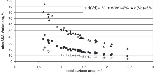
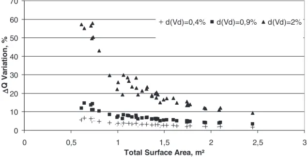
perfect thermalization is in fact quite slow, and we conclude that the main cause is cause 3, though cause 2 could occa-sionally enhance the problem in the case of very light snow. [26] An accurate measurement ofVdis crucial. Figures 5 and 6 show the simulated impacts of errors onVdon the
measured values of SA and QCH4. This was done by changing the value of Vd used in the calculations. Since
most SA values were around 1 m2, it appears that errors on
Vdare amplified at least tenfold in the final SA andQCH4 determination. In most of our measurements, the standard deviation on Vd was 0.1% or better. Therefore the
uncer-tainty on SA and QCH4 caused by errors on Vd were
usually around 1%.
[27] The importance of an accurate measurement ofVdis illustrated by the work ofHoff et al.[1998]. Those authors used a commercial volumetric apparatus to measure the SSA of fresh snow samples using N2 adsorption. They had difficulties in measuring Vd directly and estimated it by
using two different methods. In both methods, they had to neglect the closed porosity of the snow. It is well known that
Figure 5. Sensitivity of the SSA value on the error on the dead volumeVdversus sample surface area. A
snow crystals almost always contain air bubbles that reduce the density (see, e.g.,Domine´ et al.[2001]). ThusHoff et al.
[1998] overestimated Vd, which should introduce a bias in
the Q value. The sign of this bias depends on the experimental setup. This apparently significantly affected their QN2 values, which are systematically much lower than the recommended valueQN2= 2700 J/mol [Domine´ et al., 2000]. Note that measurement inaccuracies are enhanced by the use of N2rather than CH4, as detailed above.
[28] To conclude on the measurement of Vd, we found that the most reliable method was to perform repeated measurements until a stable Vd value was obtained. It is
crucial that the ambient temperature remains stable during the measurement of bothVdand the adsorption isotherm.
2.4. Reproducibility and Accuracy
[29] Tests were conducted on snow sampled at Les Deux Alpes, about 50 km ESE of Grenoble to determine the reproducibility of our method. Results are presented in Table 2. Three points were investigated.
[30] The repeatability of a measurement performed by a given experimentalist on a given sample was investigated. Experimentalist 1 performed five measurements on sample 2 and obtained a standard deviations= 1.2% on the SSA. Experimentalist 2 performed six measurements on sample 1 and obtained s= 1.4%. Repeatability is then 2s= 2.8% or better.
[31] The reproducibility of the measurement performed by two different experimentalists on the same sample was investigated. Seven samples were analyzed successively by each of the two experimentalists, yielding a reproducibility of 2s= 6.3%. We derived the reproducibility 2sas
2s¼2 ffiffiffiffiffiffiffiffiffiffiffiffiffiffiffiffiffiffiffiffiffiffiffiffiffiffiffiffiffiffiffiffiffiffiffiffiffiffiffiffiffiffiffiffiffiffiffiffiffiffiffiffiffiffiffiffiffiffiffiffiffiffiffiffiffiffiffiffiffiffiffiffiffiffiffiffiffiffiffiffiffi 1 7 X7 k¼1 SSA SSA m SSA SSA k 2! v u u t ; ð3Þ
where (SSA/SSA)k is the difference between the values
obtained by both experimentalists for samplekandSSA/
SSA)m is the mean of all (SSA/SSA)k values, which is
2.3%.
[32] These results invite two comments: (1) there is a positive correlation between the difference in Vd and the
difference in SSA measured by both experimentalists, which confirms that an accurate determination of Vd is
critical to obtain reliable results; and (2) for these measurements, special care was taken to always select the same P/P0 range, with the same number of points, and to follow the various recommendations made above as closely as possible. The value ofQCH4obtained from this data set is 2280 ± 40 J/mol, in agreement with our current recommendation. The low standard deviation supports the
Figure 6. Sensitivity of theQCH4 value on the error on the dead volumeVdversus sample surface
area.
Table 2. Summary of Reproducibility Tests
Experimentalist Sample Mass, g Vd, cm3 Q, J/mol SSA, cm2/g Total SA, m2 1 1 41.2 212.2 2294 240 0.989 2 212.8 2276 240 0.989 2 212.6 2274 238 0.981 2 212.7 2200 235 0.968 2 213.0 2244 233 0.960 2 212.7 2207 239 0.985 2 212.6 2265 235 0.968 1 2 35.8 225.7 2278 261 0.934 2 225.9 2232 266 0.952 1 225.7 2276 257 0.920 1 225.6 2305 256 0.916 1 225.6 2285 263 0.942 1 225.5 2247 264 0.945 1 3 26.9 228.4 2362 307 0.826 2 228.4 2248 311 0.837 1 4 28.1 233.6 2345 327 0.919 2 234.5 2306 317 0.891 1 5 48.1 206.6 2329 266 1.279 2 207.1 2331 256 1.231 1 6 26.5 236.0 2289 326 0.864 2 237.0 2317 307 0.814 1 7 39.2 214.4 2286 269 1.054 2 215.5 2298 255 1.000
importance of our previous recommendations, and the slightly higher value may actually be closer to the real value, but this should be confirmed by more measure-ments.
[33] To evaluate the total uncertainty on our SSA measure-ments, the contribution of systematic errors that are inherent to the BET method must also be included. The method accuracy is limited by the knowledge of the molecular surface area, by the choice of the BET linear part, and by the approximations of the BET theory, which include (1) that all the adsorbed layers but the first one are equivalent and (2) that the molecular surface area am does not depend on the
adsorbent/adsorbate and adsorbate/adsorbate interactions. FollowingGregg and Sing[1982], we estimate the system-atic uncertainty at about 10%, even though some tests on well-characterized solids showed that in some cases, system-atic errors as low as 2% could be obtained.
[34] The overall uncertainty on the SSA for a given sample is then
Total uncertainty¼pffiffiffiffiffiffiffiffiffiffiffiffiffiffiffiffiffiffiffiffiffiffiffiffiffiffiffiffiffiffiffiffiffiffiffiffiffiffiffiffiffiffiffiffiffiffiffiffiffiffiffiffiffiffiffiffiffiffiffiffiffiffiffiffiffiffiffiffiffiffiffiffiffiffiffiðReproducibility2þSystematic error2Þ
¼12%: ð4Þ
2.5. Density Measurements
[35] Density was measured as often as possible to inves-tigate SSA-density correlations. In most cases, this was done by weighing snow samples whose volumes were known by the use of a calibrated sampling volume. In this case, the accuracy is 5 to 10%, depending on the snow type. For thin surface layers (i.e., less than 5 mm) resting on hard wind-packed layers, as is often encountered in the Arctic, 400 cm2 of snow were scraped and weighted, after the thickness had been measured in about 10 spots within the 400 cm2 sampled [Domine´ et al., 2002]. The accuracy is then estimated at 15 to 20%. For very irregular or very thin layers, density could not be measured. Upper limits of density were nevertheless obtained in some of these cases by scraping snow into a calibrated volume.
3. Results
3.1. Measured Values of Snow SSA
[36] The SSA of 176 snow samples was measured: 85 were collected in the French Alps between 1998 and 2001; 58 were collected near Alert, Canadian Arctic, during the ALERT2000 campaign in February and April 2000; and 33
Table 3. SSA Values of 176 Snow Samples Classified Into 14 Types
Type Group Type SSA, cm2/g Mean SSA ±s
SSA Type
Code
Figure Freshly fallen snow Dendritic, from
Lightly rimed to graupel (Arctic, Alps) 1527, 1300, 1070, 1028, 1022, 730, 690, 666, 627 962 ± 310 F1 7a Columns, bullet combinations (Arctic,T<25C) 1460, 802, 779, 770 953 ± 340 F2 7a
Plates, needles, and columns (Alps, Arctic) 1580, 853, 840, 800, 780, 714, 700, 650, 640, 630, 620, 610, 600, 600, 600, 560, 530, 500, 470, 440, 430, 430, 400, 400, 360 629 ± 240 F3 7a Air temperature above 0C (Alps, Arctic) 672, 594, 489, 400 539 ± 120 F4 n.t.a Snow with recognizable particles Dendritic, variably rimed (Alps, Arctic) 1015, 579, 575, 540, 470, 456, 435, 410, 400, 329, 257 497 ± 200 R1 7a Columns, bullet combinations (Arctic) 770, 760, 725, 690, 690, 680, 608, 600, 570, 560, 550, 535, 530, 500, 460, 452, 444, 439, 408, 405, 404, 357, 341, 341, 326 526 ± 140 R2 7b
Plates, needles, and columns (Alps, Arctic) 670, 607, 600, 560, 500, 499, 495, 470, 450, 430, 420, 391, 376, 374, 370, 350, 340, 324, 322, 322, 317, 313, 309, 300, 290, 290, 288, 280, 270, 262, 261, 261, 257, 237, 180 373 ± 120 R3 7b
Wet snow (Alps) 550, 290 420 ± 180 R4 n.a.b
Aged snow, no more recognizable particles Mostly rounded grains (Alps, Arctic) 400, 380, 370, 280, 270, 270, 263, 252, 240, 216, 187, 168, 150, 150, 146 249 ± 80 A1 7b Mostly faceted crystals (Alps, Arctic) 231, 174, 170, 168, 161, 161, 146, 136, 134, 130, 127, 116, 113, 106, 101, 100 151 ± 50 A2 7b
Depth hoar (Arctic) 240, 200, 175, 171, 160, 150, 132, 123, 113 163 ± 40 A3 7b Melt-freeze layer
or sun crust (Alps)
300; 290; 270; 270; 260; 260; 250; 240; 240; 225; 220; 180; 134; 118
233 ± 50 A4 7b
Surface hoar (Arctic) 590; 354; 316; 315 394 ± 130 S1 7a Airborne or
recently wind-blown (Alps, Arctic)
650; 473; 408 510 ± 130 W1 n.t.a
a
Snow crystals of these types can have any shape. No typical picture exists.
b
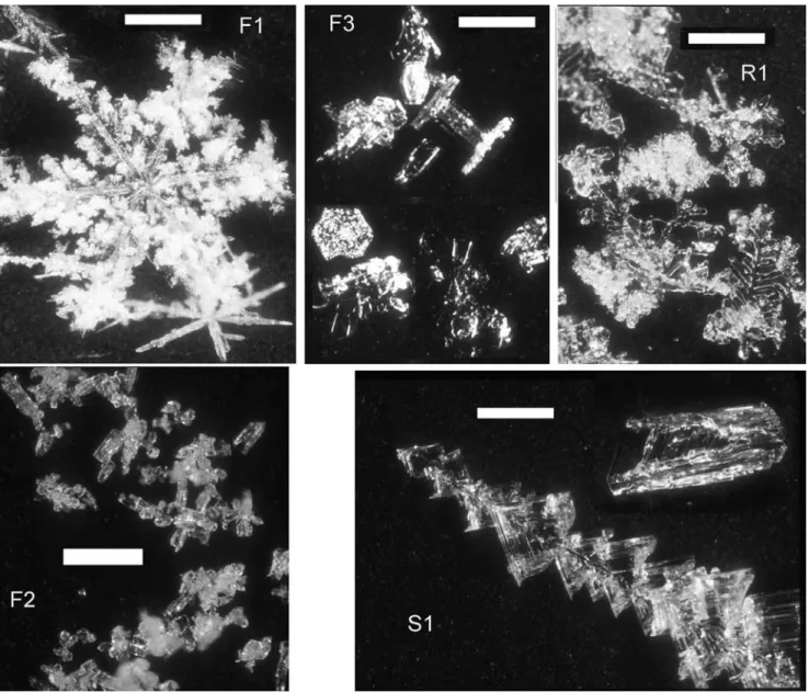
[38] The nomenclature of Table 3 and the classification used need several comments. Classifications of snow crys-tals have already been proposed bySommerfeld and LaCha-pelle [1970] and by Colbeck [1986], among others, and these should in principle be respected. However, we had difficulties applying them to our problem. For example, type I ofColbeck[1986] is ‘‘precipitation’’ and is not very detailed, while we found that dendritic snow had often higher SSA than plates or needles, and there is clearly a need for us to separate these two types. Also, we believe that it is often easier to use a classification that does not require the knowledge of the metamorphic history of the snow. The snow types chosen are therefore based on a cursory visual examination of the snow in the field, with the help of a magnifying glass. We then propose a classification with 14 types, illustrated by pictures shown in Figure 7. This classification is in no way meant to be substituted for existing ones. First of all, it is not complete, as not all snow types were encountered, and second, it is intended to be applied to our purpose, i.e., the rapid estimation in the field of the SSA of observed snow samples.
[39] The first classification criterion is the age of the snow. Freshly fallen snow is sampled within 24 hours of its fall, and usually much less. Freshly fallen snow was subdivided into dendritic snow, columns, and bullet combi-nations as are often observed in the Arctic under cold (<25C) conditions; plates, columns, and needles, ob-served in the Alps and the Arctic under moderate temper-ature conditions; and wet snow, i.e., snow falling when the air temperature was >0C. This last type includes all shapes, and this is justified by the assumption that melting removes rapidly all small structures that are expected to explain a large part of SSA variations from one type to the other. It was usually not simple to optically distinguish wet fresh snow from dry fresh snow, and the criterion actually used is the air temperature. This appears meaningful, however, as this type has the lowest mean SSA value. These four types are numbered F1 to F4 (F stands for fresh). Except for the wet character, a visual determination of these types is usually trivial. Dendritic snow in most cases had some observable rime, but no classification according to the degree of riming was attempted, as this is difficult to evaluate accurately. Cold Arctic columns and bullets never had rime. Small plates, needles, and columns usually had little or no rime. One precipitation in Svalbard consisted of heavily rimed needles that fell atT > 0C and had a SSA of 672 cm2/g. Another one consisted of a
crystals shape, which are determined by metamorphic history. Depth hoar is the result of high-temperature gra-dient metamorphism [Marbouty, 1980] and consists of large faceted crystals, with at least some of them cup-shaped and hollow. The density of this type was always <0.25. Faceted crystals are produced by metamorphism of lower temperature gradient and usually form in snow with density >0.25, that is, too high to allow depth hoar formation. Facets are clearly visible, but rounded edges were almost always present and often formed a large fraction of the visible shapes. This type contains very few or no hollow shapes. Snow with rounded grains shows a predominance of rounded shapes, but facets were almost always present, so that the border between these latter two types is not well defined and will certainly depend on the observer. Table 3 clearly shows, however, that faceted crystals have lower SSA than rounded grains. In the Arctic, snow with rounded grains had usually been hard wind-packed; grains were highly sintered and formed hard layers, sometimes so hard that even a pencil could not penetrate them. In the Alps, such snow could also be formed by low-temperature gradient metamorphism over extended periods. Finally, aged snow samples that had been subjected to melting episodes were sampled in the Alps. These four aged snow subtypes are numbered A1 to A4 (A stands for aged).
[42] Surface hoar has been classified separately (type S1, S standing for surface). It consists of readily recognizable particles that in the cases studied formed continuously, and it is therefore composed of both recent crystals and older ones. No buried surface hoar was studied. The sample with SSA = 590 cm2/g was actually hoar frost growing at Alert on antenna guy wires in February, about 2 m above the ground [Cabanes et al., 2002]. Surface hoar was forming at the same time, but much slower, and could not be sampled separately from surface snow. Photomacrographs suggest that hoar frost and surface hoar were similar in structure, and the evolution in SSA of surface snow appears consistent with the suggestion that hoar frost and surface hoar had similar SSA [Cabanes et al., 2002], but we are not entirely certain that this similarity is real. The other three surface hoar samples came from April Arctic campaigns and con-sisted of long feather-shaped crystals, as shown in Figure 7. Surface hoar formed by large clusters of hexagonal, hollow crystals were observed in the Alps but are not discussed here. Feather-shaped surface hoar is numbered S1, thus leaving room for additional types.
[43] The last type consists of snow being wind blown or very recently deposited by wind. The sample with SSA = 650 cm2/g was sampled in February at Alert while airborne, and this was done by placing a container on the snow surface, with its opening facing the wind, and letting the wind fill the container. This sample consisted of a mixture of many layers. A small fraction of the crystals could be recognized as rounded and broken surface hoar, columns, and bullets. The other samples were taken after being deposited by wind but before efficient sintering had taken place. This type is numbered W1 (W standing for wind).
[44] Table 3 clearly shows that there is a correlation between snow type and SSA and confirms our previous statement that SSA almost always decreases with time. Table 3 also shows that standard deviations are usually in the 25 to 40% range and show no trend with snow age, so that metamorphism does not seem to have a homogenizing effect.
[45] Density can also be used to facilitate the estimation of SSA. A correlation between SSA and density has already
been proposed by Narita [1971], who used stereological methods to measure SSA. However, his method was appli-cable mainly to aged snow, and very few data for fresh snow were presented. Figure 8 shows SSA versus density plots for each snow type, except for surface hoar (type S1), whose density could never be measured. Density was not measured in all cases, usually because layers were too thin. Least squares fits obtained for each snow type yielded equations (5) to (17), where d is density and where the correlation coefficient has been added (Table 4).
[46] Regarding fresh snow (types F1 to F4), only types F1 (dendritic snow) and F3 (plates, columns, and needles) have sufficient data for the correlations to be meaningful. For type F1, there is a reasonable correlation coefficient, 0.484, and using Figure 8a can lead to the estimation of the SSA of dendritic snow, knowing its density, within about 25% at the 1slevel. This relationship could be strengthened with more data, however. For type F3 (plates, needles, and columns) there is no correlation between density and SSA, and Table 3 only can be used to determine SSA, within 38%
Figure 7a. Photomacrographs of snow crystals representative of snow types F1, F2, F3, R1, and S1. Scale bars: 1 mm.
at the 1slevel. Similarly, for types F2 and F4, only the use of Table 3 is possible, but there are clearly too few data to suggest a level of confidence.
[47] Equations (9) to (11) show a weak decreasing trend of SSA with density for types R1 to R3. R4 obviously has insufficient data. The decreasing trend is visually clear for types with the most data points: dendritic snow and plates and columns. Using the plots of Figures 8c and 8d can then lead to a more accurate value than just using Table 3, and an estimation within 25 to 35% at the 1s level appears possible.
[48] Equations (13) for type A1 and (14) for type A2 indicate a significant correlation for rounded and faceted
grains, and using Figures 8e and 8f will lead to an estimation within 20 to 30% at the 1slevel. For depth hoar (equation (15)), there are insufficient data for a meaningful correlation and we recommend using Table 3, with a 25% uncertainty at the 1s level. For melt-freeze layers and sun crusts, measuring density is often delicate, as these layers are often thin. Insufficient data in Figure 8 lead to a poor correlation, and we recommend using Table 3, with a 25% uncertainty at the 1slevel. For surface hoar, note that the three values obtained in the springtime in the Arctic are within about 10% of each other, while the winter hoar frost value is much higher. Finally, both values obtained for recently wind blown snow are lower than the value of the
Figure 7b. Photomacrographs of snow crystals representative of snow types R2, R3, A1, A2, A3, and A4. Scale bars: 1 mm.
airborne snow, possibly because contact between grains and the start of the sintering process had decreased SSA, but data are too few and this is speculative.
3.2. Spatial Variability of Snow SSA
[49] Since one of the objectives of the present work is to allow the derivation of snow SSA for use in atmospheric modeling, it is crucial to test whether measurements per-formed at one location are representative of larger areas. Only limited data are presented to address this question, and the answer appears different for fresh snow and for snow that has undergone metamorphism.
[50] A preliminary test of spatial variability was made at Col de Porte (French Alps, just north of Grenoble). We collected two samples consisting of unsintered rounded
grains 1 cm under the surface of the snowpack and separated by 1 m horizontally. The measurement of their SSA was repeated by the same experimentalist 3 times for one sample and 2 times for the other one. Results indicate that the difference between both samples was 3.6%. Considering a repeatability of about 2.8% and using an equation similar to (4), we deduce that the actual SSA difference was about 2%. [51] Another test was done at Alert, where we monitored the SSA evolution of a snow layer that precipitated on 3 February 2000 [Cabanes et al., 2002] and that consisted of columns and bullet combinations. Sampling was done at two sites during 17 days: on land and on the sea ice about 7 km away. No simultaneous sampling was done at both sites. However, a plot of SSA versus time shows that the two data points obtained on the sea ice fall almost exactly
Figure 8. SSA-density correlations for the snow types of Table 3, except for surface hoar, whose density was not measured.
on the curve drawn with the six data points obtained on land [Cabanes et al., 2002], from which we infer that, for this fresh snow layer, the difference in SSA measured at both sites was less than 5%. Since the repeatability is 2.8%, the actual difference in SSA in this snow layer between two sites 7 km apart was less than 4%.
[52] A last test was performed with snow from Les Deux Alpes. We used the seven snow samples described in Table 2 that came from a layer 3 cm under the surface that had been wind blown 2 days before. Samples were taken from spots about 1 m apart. Two experimentalists measured the SSA of each sample, and the sample SSA is given as the mean value. For the whole layer, SSAlayer= 281 ± 34 cm
2 /g. The spatial reproducibility is then equal to 2s= 24% for this layer, which is only reduced to 23% if the reproducibility is taken into account. This high value may be explained by the fact that the samples were taken on an exposed slope where strong winds up to 100 km/h had blown 2 days ago. Local variations in wind effects, which include wind speed and accumulation, may therefore have resulted in different metamorphic scenarios for two adjacent spots, and this would have been enhanced by the high temperatures, which remained close to 0C during that period.
[53] From these preliminary data, we suggest that the spatial variability of fresh undisturbed snow is low, so that SSA spatial variations <5% can probably be expected, while metamorphism, including wind-induced effects, can lead to much larger spatial variations. Of course, it is clear that more extensive studies using larger data sets are needed before these numbers can be confirmed.
4. Discussion
4.1. Comparison with Other Methods and Previous Work
[54] Numerous methods can be used to measure snow SSA. Among them are stereology, grains sieving, image analysis, and the adsorption of gases other than CH4.
[55] Narita [1971] used stereology to measure snow SSA. Only his abstract is in English, and only some of the details, which are in Japanese, could be translated. He apparently studied various types of snow and plotted 113 values in a density-SSA diagram similar to ours. He divided his data into three groups according to their density (d< 0.15, 0.15 <d< 0.55, and 0.55 <d< 0.83) and performed distinct fits for these three regions, with apparently
reason-able correlation coefficients, although he had only eight points ford< 0.15. As we have no data ford> 0.55, only two of his fits are reported in Figure 8. In general, his fits indicate lower SSA values than ours, especially for fresh snow. Three possible reasons stand out: (1) fresh snow of low density sampled by Narita [1971] was already a few days old and is not of type F1 nor of type R1; (2) his method is not sensitive to small structures; indeed, his optical technique makes it difficult to take into account structures in the size range of 10mm or smaller, while CH4adsorption will detect even molecular-sized structures; hence it is not surprising to note that the higher the SSA, the greater the difference between his fits and ours; (3) accurate stereo-logical measurements require isotropy of particle location and orientation [Davis et al., 1987], which is not true for surface hoar and depth hoar and possibly also for some fresh snow types. We then suggest that for the snow types studied here, stereology will tend to underestimate SSA. A comparison using the same samples is necessary to confirm this suggestion. Stereology may be efficient to measure low SSA values, in deep firn and very dense snow, where isotropy is expected. Furthermore, such samples would have no microstructures, as these are eliminated by meta-morphism, and the systematic error that they probably cause would then not exist.Narita[1971] reports 15% uncertainty for every snow type he studied. Most of our samples had a total SA of around 1 m2. For such samples, our reproduci-bility is 6% and our accuracy is 12%. We estimate that this remains essentially true for samples with total SA of around 0.75 m2. For lower total SA, the accuracy will be reduced. Narita reports SSA values as low as 7 cm2/g, obtained when
d= 0.7. In our system, such a sample would have a total SA of 0.12 m2. Although CH4adsorption would definitely be detected, our accuracy would be 50%, at best. CH4 adsorp-tion and stereology may then be complementary techniques, to be used on different snow samples.
[56] Granberg[1985] used grain sieving to evaluate the SSA of snow samples in Quebec. Crystals were equated to spheres of equivalent radius and SSA was multiplied by 1.5 to account for nonsphericity. He obtained low SSA values between 60 cm2/g in deep snow and 200 cm2/g close to the surface. In the absence of more details on the snow studied byGranberg[1985], we cannot make any comparison with our data. However, his results do seem much lower than ours, most likely because this simple method cannot take into account microstructures.
[57] The potential of image analysis to determine SSA had been discussed at length by Domine´ et al.[2001] and has also been attempted byFassnacht et al.[1999]. A major problem with that technique is that it is extremely tedious and time consuming, even if sophisticated software is used. One SSA measurement using CH4adsorption takes 3 hours with an accuracy of 12%, while selecting and analyzing a representative number of pictures of one snow sample is much longer and only results in an accuracy of 30 to 50%. By comparison, a moderately trained eye can obtain SSA estimates with the same 30 to 50% accuracy using the data presented in Table 3 and Figure 8, and this will be rapid.
[58] Previous authors have measured the SSA of a few snow samples using N2adsorption.Adamson et al.[1967] obtained 13,000 and about 2000 cm2/g for two snow samples. TheQN2values obtained were zero or negative. According toDomine´ et al.[2000] aQN2value of around 2700 J/mol is a necessary condition for a reliable measure-ment, and these results have to be questioned. The very high values obtained also suggest that the formation of amor-phous ice of high surface area may have taken place during sample cooling. Similarly, Jellinek and Ibrahim [1967] obtained 77,700 cm2/g and QN2 = 605 J/mol for one unspecified snow sample. For the same reasons as above, this high value is certainly unreliable and perturbed by amorphous ice formation. Such a formidable value, equiv-alent to that of ice spheres of less than 1 mm in diameter, appears impossible for snow. Hoff et al. [1998] measured the SSA of six snow samples and obtained values in the range 600 to 3700 cm2/g, withQN2values in the range of 1334 – 2483 J/mol, mostly much lower than the recommen-ded value of 2700 J/mol. A low value ofQN2leads to an overestimate of SSA, and this may explain why they obtained values higher that the highest one found in this study.
[59] CH4adsorption has been used byChaix et al.[1996] and Hanot and Domine´[1999]. Chaix et al. obtained one value of 570 cm2/g for fresh snow sampled under an air temperature of – 2C. This appears consistent with type F3 snow, even though theirQCH4value was a bit low, 1919 J/ mol.Hanot and Domine´[1999] studied the evolution of the SSA of a snow layer and of surface hoar and found values in the range 22,500 to 2500 cm2/g, with a meanQCH4value of 2195 J/mol, i.e., within the range recommended here. Their values appear very high, and formation of amorphous ice during sample cooling is a clear possibility. It is troubling, however, that if such an artifact took place, it is reproducible. Two measurements on two distinct surface hoar samples yielded similar values: 2500 and 2600 cm2/g. Moreover, SSA variations show the expected trends, that have been confirmed in subsequent studies [Cabanes et al., 2002]; i.e., they decrease with time. Microstructures in the 3-mm size range are necessary to explain the high values encountered. Such small structures have been observed by
Wergin et al.[1995], but it is difficult to imagine that they could make up most of a snow sample. Hanot and Domine´ did not take photomacrographs of their samples to support their high values. Nor did they perform desorption measure-ment, to test for the presence of a hysteresis loop, as shown in Figure 4. In this study, we obtained values greater than 10,000 cm2/g twice. Each time a hysteresis loop was detected, and we realized that a leak in one of the valves
had caused the evacuation of our container before the snow was cooled, and that caused amorphous ice formation. Our preferred conclusion on the data of Hanot and Domine´ is then that amorphous ice formation probably took place. We cannot explain why their results are reproducible and the observed trends make sense. Perhaps the procedure fol-lowed was always identical, and amorphous ice formation acted as an amplification of SSA. Indeed, the flux of water vapor that will form amorphous ice is, to a first approx-imation, proportional to SSA. Of course, we are not certain that those values are not valid, but a positive confirmation of the existence of snow with such high SSA will require new measurements, whose reliability should be confirmed by the absence of a hysteresis loop and by adequate photo-graphs.
4.2. Potential Impact on Atmospheric Chemistry
[60] The impact on atmospheric chemistry of adsorption/ desorption process on snow surfaces has already been discussed in previous studies [Hanot and Domine´, 1999;
Domine´ et al., 2002;Cabanes et al., 2002]. Briefly, the total surface area (TSA) of the seasonal snowpack is a few thousand square meters per square meter of ground. At Alert, TSA values between 1160 and 3710 (dimensionless) were determined. In Svalbard near Ny-Aalesund, values between 1610 for very wind-blown coastal areas and 7600 in the upper part of the ablation zone of glaciers were estimated, as will be detailed in future publications. In the Alps, TSA values can be even higher. In the spring of 2001, the seasonal snow thickness at 3000-m elevation was 3.5 m. Using a mean density of 0.3 and a mean SSA of 250 cm2/g, the TSA was then 26,200. These values are sufficient to lead to the important sequestration of trace gases that have a moderate affinity for the ice surface, such as acetone [Domine´ et al., 2002], and the snowpack may then affect the atmospheric mixing ratios of a wide range of species.
5. Conclusion
[61] We have measured the SSA of 176 snow samples and found values between 100 and 1580 cm2/g. Snow samples were classified by age and by crystal shapes to define 14 snow types, and correlations were found between type and SSA. Using these correlations allows the estima-tion of the SSA of snow observed in the field within 40% or better at the 1s level, although more data for some snow types are needed to confirm some values. Correlations were also found between SSA and density for most snow types where sufficient data exist. Using these correlations together with the classification proposed reduces the uncertainty in SSA estimation. More measurements are required to improve our ability to estimate snow SSA, as some snow types have not been sufficiently sampled. This is the case for cold Arctic precipitation and surface hoar, for fresh or recent wet snow, and for recently wind-blown snow. The method proposed here appears reproducible (6%) and accu-rate (12%) and is more rapid than image analysis. We argue that for snow with SSA greater than about 100 cm2/g, which includes all the seasonal snow samples studied here, our method may be more accurate than stereology, because it detects the tiniest details. For older snow with lower SSA, and whose small structures have been removed by
meta-References
Adamson, A. W., L. M. Dormant, and M. Orem, Physical adsorption of vapors on ice, I, Nitrogen,J. Colloid Interface Sci.,25, 206 – 217, 1967. Barrie, L. A., J. W. Bottenheim, P. J. Schnell, P. J. Crutzen, and R. A. Rasmussen, Ozone destruction and photochemical reactions at polar sun-rise in the lower Arctic atmosphere,Nature,334, 138 – 141, 1988. Brunauer, S., P. H. Emmet, and E. Teller, Adsorption of gases in
multi-molecular layers,J. Am. Chem. Soc.,60, 309 – 319, 1938.
Brunauer, S., L. S. Deming, W. E. Deming, and E. Teller, On a theory of the van der Waals adsorption of gases,J. Am. Chem. Soc.,62, 1723, 1940. Cabanes, A., L. Legagneux, and F. Domine´, Evolution of the specific sur-face area and of crystal morphology of fresh snow near Alert during ALERT 2000 campaign,Atmos. Environ.,36, 2767 – 2777, 2002. Chaix, L., J. Ocampo, and F. Domine´, Adsorption of CH4on
laboratory-made crushed ice and on natural snow at 77 K: Atmospheric implications,
C. R. Acad. Sci., Ser. II,322, 609 – 616, 1996.
Colbeck, S. C., Classification of seasonal snow cover crystals,Water Re-sour. Res.,22, 59S – 70S, 1986.
Couch, T. L., A.-L. Sumner, T. M. Dassau, P. B. Shepson, and R. E. Honrath, An investigation of the interaction of carbonyl compounds with the snowpack,Geophys. Res. Lett.,27, 2241 – 2244, 2000.
Davis, R. E., J. Dozier, and R. Perla, Measurement of snow grain proper-ties, inSeasonal Snowcovers,NATO ASI Ser. C211, pp. 63 – 74, N. Atl. Treaty Organ., Brussels, 1987.
Dibb, J., et al., Air-snow exchange of HNO3and NOyat Summit, Green-land,J. Geophys. Res.,103, 3475 – 3486, 1998.
Domine´, F., and E. Thibert, Mechanism of incorporation of trace gases in ice grown from the gas phase,Geophys. Res. Lett.,23, 3627 – 3630, 1996. Domine´, F., L. Chaix, and L. Hanot, Reanalysis and new measurements of N2and CH4adsorption on ice and snow,J. Colloid Interface Sci.,227,
104 – 110, 2000.
Domine´, F., A. Cabanes, A.-S. Taillandier, and L. Legagneux, Specific surface area of snow samples determined by CH4adsorption at 77 K,
and estimated by optical microscopy and scanning electron microscopy,
Environ. Sci. Technol.,35, 771 – 780, 2001.
Domine´, F., A. Cabanes, and L. Legagneux, Structure, microphysics, and surface area of the Arctic snowpack near Alert during ALERT 2000,
Atmos. Environ.,36, 2753 – 2765, 2002.
Fassnacht, S. R., J. Innes, N. Kouwen, and E. D. Soulis, The specific surface area of fresh dendritic snow crystals,Hydrol. Processes, 13, 2945 – 2962, 1999.
Frei, A., and D. A. Robinson, Evaluation of snow extent and its variability in the Atmospheric Model Intercomparison Project,J. Geophys. Res.,
103, 8859 – 8871, 1998.
firn transfer studies of HCHO at Summit, Greenland,Geophys. Res. Lett.,
26, 1691 – 1694, 1999.
Jellinek, K., and S. Ibrahim, Sintering of powdered ice,J. Colloid Interface Sci.,25, 245 – 254, 1967.
Klinger, J., and J. Ocampo, Apparent solubility of helium in snow and ice,
J. Phys. Chem.,87, 4114, 1983.
Kouchi, A., et al., Conditions for condensation and preservation of amor-phous ice and astrophysical ices,Astron. Astrophys.,290, 1009 – 1018, 1994.
Marbouty, D., An experimental study of temperature gradient metamorph-ism,J. Glaciol.,26, 303 – 312, 1980.
Mayer, E., and R. Pletzer, Amorphous ice, a microporous solid: Astrophy-sical implications,J. Phys.,48, C1-581 – C1-586, 1987.
Michalowski, B. A., J. S. Francisco, S.-M. Li, L. Barrie, J. W. Bottenheim, and P. Shepson, A computer model study of multiphase chemistry in the Arctic boundary layer during polar sunrise, J. Geophys. Res., 105, 15,131 – 15,145, 2000.
Narita, H., Specific surface of deposited snow, II,Low Temp. Sci.,A29, 69 – 81, 1971.
Peterson, M. C., and R. E. Honrath, Observations of rapid photochemical destruction of ozone in snowpack interstitial air,Geophys. Res. Lett.,28, 511 – 514, 2000.
Robinson, D. A., K. F. Dewey, and R. R. Heim Jr., Global snow cover monitoring: An update,Bull. Am. Meteorol. Soc.,74, 1689 – 1696, 1993. Sommerfeld, R. A., and E. LaChapelle, The classification of snow
meta-morphism,J. Glaciol.,9, 3 – 17, 1970.
Sumner, A. L., and P. B. Shepson, Snowpack production of formaldehyde and its effect on the Arctic troposphere,Nature,398, 230 – 233, 1999. Thibert, E., and F. Domine´, Thermodynamics and kinetics of the solid
solution of HNO3in ice,J. Phys. Chem. B,102, 4432 – 4439, 1998.
Weller, R., A. Minikin, G. Ko¨nig-Langlo, O. Schrems, A. E. Jones, E. W. Wolff, and P. S. Anderson, Investigating possible causes of the observed diurnal variability in Antarctic NOy,Geophys. Res. Lett.,26, 601 – 604, 1999.
Wergin, W. P., A. Rango, and E. F. Erbe, Observations of snow crystals using low-temperature scanning electron microscopy,Scanning,17, 41 – 49, 1995.
A. Cabanes, F. Domine´, and L. Legagneux, Laboratoire de Glaciologie et Ge´ophysique de l’Environnement, CNRS, BP 96, 38402 St. Martin d’He`res, Cedex, France. ([email protected])