Behavioral/Systems/Cognitive
Trade-Off between Object Selectivity and Tolerance in
Monkey Inferotemporal Cortex
Davide Zoccolan, Minjoon Kouh, Tomaso Poggio, and James J. DiCarlo
McGovern Institute for Brain Research, Department of Brain and Cognitive Sciences, Center for Biological and Computational Learning, Massachusetts Institute of Technology, Cambridge, Massachusetts 02142
Object recognition requires both selectivity among different objects and tolerance to vastly different retinal images of the same object, resulting from natural variation in (e.g.) position, size, illumination, and clutter. Thus, discovering neuronal responses that have object selectivity and tolerance to identity-preserving transformations is fundamental to understanding object recognition. Although selectivity and tolerance are found at the highest level of the primate ventral visual stream [the inferotemporal cortex (IT)], both properties are highly varied and poorly understood. If an IT neuron has very sharp selectivity for a unique combination of object features (“diagnostic features”), this might automatically endow it with high tolerance. However, this relationship cannot be taken as given; although some IT neurons are highly object selective and some are highly tolerant, the empirical connection of these key properties is unknown. In this study, we systematically measured both object selectivity and tolerance to different identity-preserving image transformations in the spiking responses of a population of monkey IT neurons. We found that IT neurons with high object selectivity typically have low tolerance (and vice versa), regardless of how object selectivity was quantified and the type of tolerance examined. The discovery of this trade-off illuminates object selectivity and tolerance in IT and unifies a range of previous, seemingly disparate results. This finding also argues against the idea that diagnostic conjunctions of features guarantee tolerance. Instead, it is naturally explained by object recogni-tion models in which object selectivity is built through AND-like tuning mechanisms.
Key words:inferotemporal cortex; monkey; object recognition; multiple objects; trade-off; tolerance
Introduction
The key computational problem of object recognition is attaining both selectivity among different visual objects and tolerance to variation in each object’s appearance (e.g., as a result of changes in position, size, illumination, clutter, etc.). The primate visual system has solved this problem: primates robustly and effortlessly discriminate among visual objects over the wide range of images that each object produces during natural vision (Potter, 1976; Intraub, 1980; Rubin and Turano, 1992; Logothetis and Shein-berg, 1996; Thorpe et al., 1996; Edelman, 1999; Rousselet et al., 2004). What neuronal architecture and computations create such a selective and tolerant representation of visual objects? Because previous work indicates that these properties are built by a hier-archy of cortical stages (the ventral visual stream) (Logothetis and Sheinberg, 1996; Tanaka, 1996; Rolls, 2000; Rousselet et al., 2004), experimental studies can shed light on this question by
examining the strength, variation, and relationship of object se-lectivity and tolerance across the ventral visual stream.
Here we focus on the culmination of the ventral visual stream, the anterior portion of the inferotemporal cortex (IT). Although object selectivity and tolerance are found in IT, these properties are highly varied both within and across studies (Logothetis and Sheinberg, 1996; Tanaka, 1996; Rolls, 2000; Rousselet et al., 2004), and their connection at the level of single IT neurons is not understood. One possibility is that, as signals propagate through the visual system, neurons become highly selective for unique combinations of features that also guarantee high tolerance to identity-preserving transformations of those features. This no-tion derives from the grandmother or gnostic cell concept of Lettvin and Konorski (Gross, 2002), and has been recently invig-orated by the observation that some neurons in the human me-dial temporal lobe (Quiroga et al., 2005) respond only to specific visual objects regardless of size, pose, and visual clutter. This notion also seems consistent with previous physiological results: sharpness of object selectivity and tolerance (e.g., to position or size changes) both increase along the ventral visual stream (Ko-batake and Tanaka, 1994; Logothetis and Sheinberg, 1996; Tanaka, 1996; Edelman, 1999; Rolls, 2000; Rousselet et al., 2004). Nevertheless, however appealing, this notion cannot be taken as given; we do not yet know whether individual IT neurons attain high values of both selectivity and tolerance. More generally, we do not even know whether these properties are connected in any Received April 26, 2007; revised Sept. 20, 2007; accepted Sept. 24, 2007.
This work was supported primarily by the National Institutes of Health. Additional support was provided by Defense Advanced Research Projects Agency, Office of Naval Research, The Pew Charitable Trusts, The McKnight Foundation, Eastman Kodak Company, Honda Research Institute, Siemens Corporate Research, Sony, and the Mc-Dermott chair (T.P.). D.Z. was supported by a Postdoctoral Fellowship of The International Human Frontier Science Program Organization and by a Charles A. King Trust Postdoctoral Research Fellowship. We thank J. Maunsell, N. Li, and N. Rust for comments on this manuscript; D. Cox, T. Serre, and G. Kreiman for discussion; C. Hung for help in stimulus preparation; and J. Deutsch for technical support.
Correspondence should be addressed to James J. DiCarlo, McGovern Institute for Brain Research, Massachusetts Institute of Technology, 77 Massachusetts Avenue, Cambridge, MA 02139. E-mail: [email protected].
DOI:10.1523/JNEUROSCI.1897-07.2007
Copyright © 2007 Society for Neuroscience 0270-6474/07/2712292-16$15.00/0 12292•The Journal of Neuroscience, November 7, 2007•27(45):12292–12307
way, because no study has systematically measured both proper-ties in the same IT neuronal population.
To address this issue, we systematically measured both object selectivity and tolerance to different identity-preserving image transformations within the same IT neuronal population in two monkey subjects engaged in a simple object detection task. For each neuron, we measured (1) how selectively it responded across a large object set (object selectivity) (see Fig. 1A, top); and (2) how well preserved its response was to a very effective reference object that underwent different transformations: position, size, and contrast changes and addition of visual clutter (absolute tol-erance) (see Fig. 1A, bottom). Although another way to measure tolerance is to check how well relative object preference is pre-served across transformations (relative tolerance) (Tovee et al., 1994; Ito et al., 1995), we focused here on absolute tolerance of neuronal responses because it provides a bound on other toler-ance metrics and measures the ability of individual neurons to support recognition without further processing (see Discussion). Contrary to the appealing idea that IT contains neurons that are both highly shape selective and highly tolerant, we discovered that selectivity and tolerance trade off across the IT population: neurons with high object selectivity typically have relatively low tolerance, and vice versa.
Materials and Methods
We used standard procedures for surgical preparation, behavioral task and training, eye position monitoring, and single-unit electrophysiolog-ical recording in awake monkeys, and details are described by Zoccolan et al. (2005). Here we briefly describe those methods that are most relevant to the present study. All animal procedures were performed in accord with National Institute of Health guidelines and the Massachusetts Insti-tute of Technology Committee on Animal Care.
Visual stimuli and behavioral task
All recorded neurons were probed with a fixed set of 213 grayscale pic-tures of isolated real-world objects, mostly modified from the Caltech 101 database (Fei-Fei et al., 2004), but including also (1) five fixed object prototypes from each of three spaces of parameterized objects (see be-low); (2) five patches of texture; (3) four low-contrast images of one of the objects; and (4) a blank frame (used to measure neuronal background rate). The full set is shown in supplemental Figure 1 (available at www. jneurosci.org as supplemental material). Some neurons were also tested using additional objects drawn from the three spaces [cars, faces, and two-dimensional (2-D) silhouettes] with parametrically controllable shape similarity within each space. Each object space consisted of 14 morph axes (for a total of 42 morph axes), and each morph axis was composed of five shapes resulting from blending two object prototypes (e.g., two car brands) in different proportions (see examples in Fig. 2B) (for details, see Zoccolan et al., 2005). All objects subtended⬃2°.
During recordings, both monkeys were engaged in a simple recogni-tion task that required the detecrecogni-tion of a fixed, red target shape (a red triangle) that was presented at the end of a temporal sequence of object conditions drawn from our stimulus set (see Fig. 1B). The total number of stimulus conditions presented on each behavioral trial ranged from 3 to 20. The target was always the last in the sequence, and each monkey was rewarded for maintaining fixation (⫾1.5° fixation window) until the appearance of the target and then making a saccade to a fixed visual field location (7° eccentricity) within 800 ms after the appearance of the target. The size of the fixation window was chosen to be small enough to guarantee that the monkeys could not make a saccade to any of the eccentric positions that were tested during the mapping of the receptive field (RF) (see below) without leaving the fixation window and, there-fore, aborting the trial. This was guaranteed by the fact that the closest positions to fixation were⫾2.5° from the fixation spot (see below), i.e.,
⫾1° beyond the edge of the fixation window.
Single objects from the fixed stimulus set and identity-preserving transformations of a very effective reference object (see Fig. 1A) were
pseudorandomly interleaved. Visual stimuli were presented at a rate of 5 per second; i.e., each stimulus condition was shown for 100 ms, followed by 100 ms of a gray screen (no stimulus), followed by another stimulus condition for 100 ms, etc. (see Fig. 1B). This task was meant to obtain a large amount of data, while still engaging the animal in a recognition task. We have previously shown that clutter suppression during such tasks is not simply explained by variation in spatial attention (Zoccolan et al., 2005).
Neuronal recordings
During each recording session, a single extracellular metal electrode was advanced into IT. Over⬃6 months of daily recording sessions in the two monkeys, we sampled neurons over an⬃5⫻4 mm area of the ventral superior temporal sulcus and ventral surface lateral to the anterior mid-dle temporal sulcus (Horsey-Clark coordinates: anteroposterior, 13–17 mm; 18 –21 mm mediolateral at recording depth).
Screening procedures. Each isolated neuron was tested for responsive-ness across the fixed set of 213 stimuli plus 30 additional object proto-types belonging to the parameterized morphed spaces (Zoccolan et al., 2005) using a very inclusive criterion: a neuron was considered respon-sive if its mean firing rate was significantly higher than background rate for at least one of these stimuli (ttest,p⬍0.005, which impliesp⬍0.7 corrected for multiple tests). All stimuli were presented at the center of gaze. Two to four presentation repetitions were collected for each stim-ulus. This screening procedure was used to identify a very effective ref-erence object (the object that produced the strongest neuronal response, higher than background rate according to thettest) and six poorly effec-tive flanking objects (the objects that produced the smallest response, not significantly higher than background rate according to thettest). Note, however, that, because of trial-by-trial noise, in the final testing in which more repetitions were used (see below), the chosen objects did not always turn out to be the most effective (and ineffective) objects. Only respon-sive neurons for which these reference and flanking objects could be found were selected for further testing and recordings. The screening procedure was also used to decide whether the neuron was responsive to any of the object prototypes belonging to the parameterized morphed spaces (a total of 45 prototypes were used, 15 of which belonged to the fixed set of 213 visual stimuli; see above).
If selected for recordings (see above), a neuron was further screened to identify its preferred receptive field location (RF center) within a narrow span of visual angle around the center of gaze. Our goal was not to map each neuron RF over the whole visual field, but rather to optimize the location in which to present our single object conditions during the main testing session (see below). To achieve this, the most effective (reference) object and the least effective object were presented over a span of 2° around the fixation spot (8 –10 repetitions). More specifically, six visual field locations (in addition to fixation) were tested. Four of these loca-tions were the extremes of a “cross” centered on fixation (i.e., 2° above and below fixation and 2° left and right to fixation). The other two locations were⫾2° in elevation and 2° in azimuth, in the contralateral hemifield with respect to the recording chamber. The visual field location in which the response produced by the reference was higher was chosen as RF center of the neuron. Within this 2° span, most neurons (75/94) had their RF center at the center of gaze.
Recording session.Complete recordings were obtained from each neu-ron using pseudorandomly interleaved stimuli from our entire battery of stimulus conditions: (1) single objects belonging to the fixed object set and presented in the neuron’s RF center (see Fig. 1A, broad sampling); (2) identity-preserving transformations of the reference object to test clutter tolerance (CT), position tolerance (PT), size tolerance (ST), and contrast tolerance (CrT) (see Fig. 1A). If the neuron was responsive to any of the 45 morphed object prototypes that were probed during screen-ing (see above), it was also tested with five objects belongscreen-ing to the morph axis that included the effective object prototype (see Fig. 1A, local sampling).
Tolerance to position changes was assessed by mapping the response to the reference object across a vertical⬃12° span of visual field (see Fig. 3A). The reference object was presented in the RF center (see above) and in eight additional positions: (1)⫺2.5° below the RF center; and (2) 2.5,
3.5, 4.5, 5.5, 7.5, 9.5, and either 11 (73/94 cells) or 12° (21/94 cells) above the RF center. Position tolerance was not mapped in full 2-D space be-cause it would have been too time consuming (see below). Based on results in the literature (Tovee et al., 1994; Ito et al., 1995; Op De Beeck and Vogels, 2000), our testing should provide a reasonable estimate of position tolerance, and we have no reason to believe that a full 2-D map of the RF field would lead to qualitatively different results.
Tolerance to size changes was measured by presenting the reference object at four different sizes (1, 2, 4, and 6°) at the RF center (see Fig. 3B). Object conditions to measure ST were tested for all neurons from mon-key 2 (n⫽34) but only for a subset of neurons from monkey 1 (18/60). Tolerance to contrast changes was assessed by presenting the reference object at three low contrasts (1.5, 2, and 3%), in addition to its default contrast (mean default contrast across reference objects⫾SD⫽33⫾ 12%), at 2.5° above the RF center (see Fig. 3C). The reason that contrast tolerance was not measured at the RF center is that the data presented in this study are part of a larger experimental design, in which, among other things, the relationship between clutter tolerance and the contrast of the flanker objects was tested. To measure such a relationship, flankers at different low contrasts were presented 2.5° above the RF center. To save time (see below), the same low-contrast conditions were not presented also at the RF center. Stimulus contrast was defined as follows: [med
(pix⬎Lbackground)⫺med(pix⬍Lbackground)]/[med(pix⬎Lbackground)
⫹med (pix⬍Lbackground)], where med indicates the median taken over
the pixel values either above or below the monitor background lumi-nance level (Lbackground).
To test clutter tolerance, the reference object was presented both in isolation and along with each of the six, poorly effective flanking objects (see above) (see Fig. 3D). Objects in the pairs used to test clutter tolerance were 2.5° apart (center to center), with the effective reference object in the neuron RF center and the flanking object located 2.5° either above or below the RF center.
As described above, given the time limitations of awake recording, only a limited amount of object conditions could be used to measure each tolerance property. Therefore, our goal was not to obtain the best possi-ble estimate of each tolerance property per se, but rather to collect enough data to understand how these properties covaried with object selectivity and with each other.
The transformations of the reference object described above allow measuring the absolute tolerance of each neuron, i.e., how well preserved the response to the effective reference object across each transformation (see below for a definition of the tolerance metrics) is. Alternatively, tolerance can be defined in terms of how well preserved the rank order of object selectivity across the tested transformations (relative tolerance) is. Although our study was not meant to provide an accurate estimate of relative tolerance (see Introduction and Discussion), in addition to mea-suring how the response to the effective reference object changed by varying its position, size, and contrast, we also measured how these same transformations affected the response to a very ineffective object (one of the flanking objects). This allows a first-order assessment of relative tol-erance across the recorded population (see below).
Five to thirty presentation repetitions were collected for each object condition (see supplemental material 1.B for details, available at www.jneurosci.org).
Data analysis
Choice of the spike count window.To get the most statistical power from the data, average firing rates were computed over a time window (relative to stimulus onset) whose extremes were optimally chosen for each neu-ron by an apposite algorithm. Briefly, epochs of the neuneu-ronal response were identified in which the background corrected response was at least 20% of its peak value. If multiple such epochs existed, they were merged to the epoch containing the response peak if they were within 25 ms from it. This algorithm is completely described in supplemental material 1.A and supplemental Figure 2 (available at www.jneurosci.org as supple-mental material). Analyses performed using either such neuron-specific spike count windows (mean onset across neurons⫾SD⫽101⫾18 ms; mean offset⫽236⫾48 ms) or count windows that were held fixed across the recorded neuronal population yielded very similar results
(supple-mental Tables 1, 2, available at www.jneurosci.org as supple(supple-mental ma-terial). The neuron-specific spike count windows were used to estimate latency and duration of the neuronal responses in the analysis shown in supplemental Table 6 (available at www.jneurosci.org as supplemental material). For such analysis, onset and offset of the response were com-puted considering epochs in which the background corrected response was at least either 20% (as for our standard spike count window) or 10% (for a better comparison with previous studies) (Brincat and Connor, 2006) of its peak value.
To assess the dependency of the selectivity and tolerance properties (see below) from the time course of the neuronal response, firing rates were also computed in overlapping time windows of 50 ms shifted in time steps of 25 ms (see Fig. 6).
Analyses were performed using absolute firing rates, but very similar results were obtained when driven (i.e., “background subtracted”) rates were used (supplemental Tables 1, 2, available at www.jneurosci.org as supplemental material).
Selectivity and tolerance metrics.The selectivity of each neuron across the fixed set of 213 stimuli was quantified by the sparseness of its response (Rolls and Tovee, 1995a; Vinje and Gallant, 2000; Olshausen and Field, 2004):S⫽{1⫺[(⌺Ri/n)2/⌺(Ri2/n)]}/[1⫺(1/n)], whereRiis the
neu-ron response to theith stimulus andnis the number of stimuli in the set.
Sranges from 0 (no object selectivity) to 1 (maximal object selectivity). Neuronal selectivity within each morphed set was quantified by the fol-lowing morph tuning index (Rainer et al., 1998): MT⫽[n⫺(⌺Ri/
Rmax)]/(n⫺1), whereRiis the neuron response to theith morphed object,Rmaxis the maximal response within the morphed set, andnis the number of objects in the set. As sparseness, MT ranges from 0 (no shape selectivity) to 1 (maximal shape selectivity).
For each neuron, PT was defined as two times the SD of the Gaussian function that best fitted the normalized driven rates across the tested RF positions. Operationally, we subtracted the background activity from the neuron responses across the tested RF positions, and we normalized (1.0) the resulting RF profile. Then, we fit a Gaussian function to the RF profile, with the peak of the Gaussian centered on the peak of the RF. As a goodness-of-fit measure, we used the sum of the absolute residuals SR. Only neurons such that SR⬍1.5 were included in the analyses presented throughout the paper. For the analysis shown in Figure 5C(top left), only neurons such that SR⬍0.8 were included in the population-averaged RF profiles, to guarantee that only RFs with homogeneous shapes (i.e., all strictly Gaussian) contributed to the average. Note that in Figure 5C(see legend), before being averaged, the receptive field profiles were aligned to the position (elevation) of their peak values. Because the tested elevations were not located in an equally spaced grid (see above), aligning the peaks produces a misalignment of the elevations at which each neuron was tested. Thus the RF profiles in Figure 5Cwere averaged in overlapping windows of⬃3°, shifted in steps of⬃1°. Depending on what elevations fell in a given averaging window, the average elevation in that window may be different between subpopulations.
ST was quantified by normalizing (1.0) the size tuning curves to their maximal values (see Fig. 3B, bottom) and then averaging the resulting tuning curve values that were⬍1, i.e., ST⫽冓Rtest size/max(Rtest size)冔,
where Rtest size is the mean response to a given tested size of the
reference object, and 冓䡠冔 is the average over the sizes such that
Rtest size⬍max(Rtest size). Contrast tolerance (CrT) was similarly
mea-sured, but after normalizing each contrast tuning curve to the original contrast of the reference object (see Fig. 3C, bottom, leftmost point), i.e., CrT⫽冓Rtest contrast/Rref contrast冔, whereRtest contrastis the mean response to
a given tested contrast of the reference object,Rref contrastis the mean
response to the reference object presented at its original contrast, and冓䡠冔is the average over the tested contrasts (3, 2, and 1.5%) (see Fig. 3D). ST and CrT measure the amount of response that is preserved, on average, when the reference object is transformed by changing, respectively, its optimal size or its reference contrast. Both metrics range between 0 (no tolerance) and 1 (complete invariance).
We quantified the clutter tolerance of each neuron with the following clutter tolerance (CT) metric: CT⫽冓(Rref & flanker⫺Rflanker)/(Rref⫺
Rflanker)冔, whereRref & flankeris the mean response to a given pair
refer-ence/flanker,RrefandRflankerare the mean responses to the constituent
objects of that pair (i.e., the reference and flanker objects presented alone), and冓䡠冔is the average over the included flanker conditions (for most analyses, only flankers such thatRflanker⬍50%Rrefor less were
considered) (but see Fig. 7A). CT values near 0 indicate very poor clutter tolerance (strong suppression by flanker objects), whereas values near 1 indicate complete clutter invariance (CCI; no effect of flanker objects). CT⬎1 indicates facilitation by clutter. It is important to note that, because the response to the isolated flanker objects is subtracted from
bothRref & flankerandRrefin the definition of CT, the metric is unbiased
with respect to either a CCI or a clutter averaging rule (Zoccolan et al., 2005) (see Fig. 7Afor details).
Significance and SE of the correlation coefficients reported through this manuscript were computed, respectively, using a one-tailed permu-tation test (5000 samples) and bootstrap analysis (500 samples).
Presentation repetitions of the reference object were split to guarantee complete independence of the datasets over which selectivity and toler-ance metrics were computed (see supplemental material 1.B, available at www.jneurosci.org). The number of neurons included in the different analyses presented throughout the paper (see Figs. 4 –7; supplemental Tables 1–3, available at www.jneurosci.org as supplemental material) was selected according to specific criteria that are fully described in sup-plemental material 1.C (available at www.jneurosci.org).
To obtain a measure of the relative tolerance of object selectivity across the tested transformations, for each of the position, size, and contrast changes, we computed the difference between the response (average fir-ing rate) to the effective reference object (Rref) and the response to one of
the poorly effective flanker objects (Rflanker), normalized by the mean of
the standard deviations (refandflanker) of the two response rates. In
other words, we computed ad⬘index, defined as follows:d⬘ ⫽(Rref⫺
Rflanker)/, with⫽(ref⫹flanker)/2. This index tells how far apart the
responses to the effective and ineffective objects are. Negative values indicate that, for a given transformation, the tuning of the neuron has reversed (i.e., the ineffective flanker produced a response larger than the effective reference).
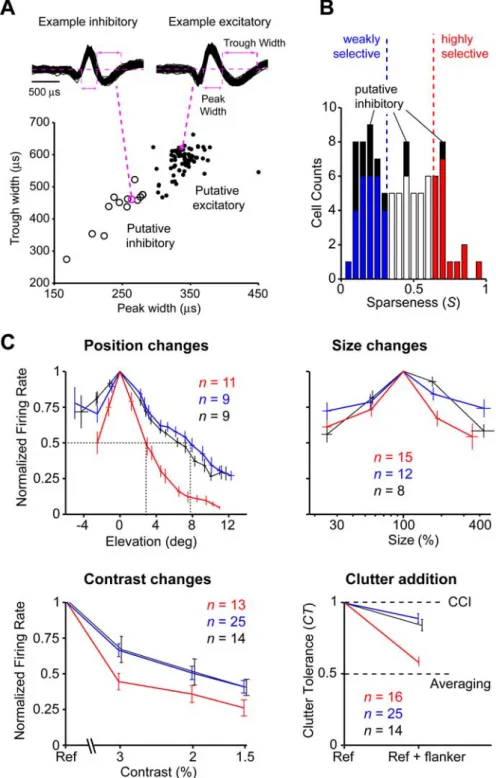
Spike waveform analysis.Putative inhibitory and excitatory neurons were identified across the recorded neuronal population based on the waveform of the action potentials collected for each cell. Previous studies
performed in cortical slices and anesthetized animals (McCormick et al., 1985; Connors and Gutnick, 1990; Nowak et al., 2003) and addi-tional studies based on cross-correlation analy-sis of spike trains (Bartho et al., 2004; Tamura et al., 2004) have shown the reliability of such an approach in identifying neuronal typing. As a consequence, many authors have distinguished between putative excitatory and inhibitory neu-rons recorded in different brain areas of awake animals (such as hippocampus, somatosensory cortex, lower and higher visual cortical areas, and rat barrel cortex) using only the temporal features of the spike waveforms (Mountcastle et al., 1969; Gur et al., 1999; Frank et al., 2001; Bruno and Simons, 2002; Andermann et al., 2004; Mitchell et al., 2007). In this study, fol-lowing Bruno and Simons (2002), two compo-nents of the waveform were taken as distinctive features of the neuron type: (1) the duration (width) of the central peak (negative or posi-tive); and (2) the width of the following trough (corresponding to the spike afterhyperpolariza-tion). Figure 5Ashows a scatter plot with the mean width of the peak and trough for our pop-ulation of 94 neurons. The cluster of neurons with shorter mean widths (empty circles) was identified as putative inhibitory. The cluster with longer mean widths (filled circles) was des-ignated as excitatory. Waveforms of one exam-ple neuron from each cluster are shown in Figure 5A(top).
Monte Carlo simulations to check that the sparseness and clutter tolerance metrics are not implicitly correlated.Monte Carlo simulations were run to check that the inverse relationship be-tweenSand CT (see above) could not arise by chance as the result of an implicit correlation between these metrics computed over a population of noisy neuronal responses (see Fig. 7B). For any given neuron, re-sponses to the single object conditions were simulated using Poisson spike generators with mean rate equal to the actual mean firing rate that was recorded for each single object condition (the same number of rep-etitions collected for each object condition were simulated). The selec-tivity (sparseness,S) of each neuron was computed based on these Pois-son simulated responses to single objects. A simulated response to clutter (i.e., to the tested object pairs) was implemented either assuming an averaging rule or assuming CCI. Two versions of the averaging rule were implemented: (1) one exact, i.e.,Rref & flanker⫽0.5 (Rref⫹Rflanker); (2)
the other approximate, i.e., withRref & flankerrandomly sampled between
Rflanker andRref(in both cases, Poisson statistics of spike trains were
assumed). The CT of each neuron was computed based on these Poisson simulated responses to object pairs. Each Monte Carlo simulation was repeated 500 times, yielding the null distributions of regression lines and correlation coefficients shown in Figure 7B.
Model simulations
The hierarchical object recognition model used to generate Figure 9Eis fully described in previous reports (Riesenhuber and Poggio, 1999; Serre et al., 2005, 2007a,b). See supplemental material 2 and supplemental Figure 7 (available at www.jneurosci.org as supplemental material) for details about model simulations and additional modeling results.
Results
To examine the relationship between object selectivity and toler-ance in IT, we performed extracellular microelectrode recordings in two monkeys that viewed grayscale images of real-world ob-jects presented at a rate of 5 images/s, while the animals were engaged in a simple object detection task (Fig. 1B) (see Materials and Methods). Well isolated neurons were randomly sampled Figure 1. Rationale of the experimental design and behavioral task.A, For each neuron, we measured (1) its object selectivity,
i.e., its sensitivity to changes in object identity (measured both across a large set of real-world objects, and, when possible, across local, parameterized sets of morphed shapes); and (2) its tolerance to different identity-preserving image transformations of an effective reference object.B, During recordings, monkeys were presented with rapid sequences of pseudorandomly interleaved grayscale objects used to measure selectivity and tolerance (see above). The monkey’s task was to respond to the red triangle at the end of each sequence. The number of objects presented before the triangle was random (between 3 and 20).
throughout anterior IT and tested for responsiveness across a fixed, large set of visual objects (see Materials and Methods). Each responsive neuron was then tested with a battery of object con-ditions to measure (1) its object selectivity, i.e., its sensitivity to changes in object identity (Fig. 1A, top); and (2) its tolerance to different identity-preserving transformations of a reference ob-ject, including position, size and contrast changes, and presence of clutter (Fig. 1A, bottom). Complete recordings were obtained from 94 IT neurons (60 in monkey 1, 34 in monkey 2). We took special care to obtain independent data and design independent metrics for selectivity and tolerance so as to guarantee no implicit relationship among these properties (see Materials and Methods and supplemental material 1B, available at www.jneurosci.org). Broad range of object selectivity across the IT
neuronal population
To get a first-order measure of each neuron’s object selectivity, we estimated the fraction of objects in a large, fixed set of 213 stimuli (see supplemental Fig. 1, available at www.jneurosci.org as supplemental material, Fig. 2A) that produced a response (sparseness, described immediately below). For most neurons (see Materials and Methods), we also measured shape selectivity within several predefined parameterized object shape spaces (Fig. 2B, morph tuning, described in detail later in Results) (see also
Zoccolan et al., 2005). Both methods uncovered a remarkably broad spectrum of sensitivity to shape changes within IT. For example, although many neurons responded strongly to their preferred object within the fixed shape set (population mean⫾ SD⫽49.5⫾21.2 spikes/s) (see supplemental Fig. 5, available at www.jneurosci.org as supplemental material), the population was highly varied in the number of objects that elicited a strong response. This can be visually appreciated by ranking, for each neuron, the 213 test stimuli based on the response they evoked (Fig. 2A, bottom). For example, some neurons were weakly se-lective in that they showed a strong response to many objects [Fig. 2A, blue curve and peristimulus time histograms (PSTHs)]. Other neurons were highly selective in that they responded well to only a handful of objects (Fig. 2A, red curve and PSTHs). These example neurons illustrate the broad range of selectivity seen across the IT population (Fig. 2A, gray lines). Note however, that even the least-selective neurons within our IT population typically showed some (nonzero) object selectivity in that some objects elicited little or no response (Fig. 2A). In fact, all neurons that fired at least 10 spikes/s to the effective reference object (see Materials and Methods) and were included in further analyses (91/94 cells), responded significantly more to the reference object than to one of the weakly effective flanker objects chosen during Figure 2. Broadness of object selectivity in IT.A, Normalized firing rate profiles (bottom) across a fixed set of 213 objects for a population of 94 neurons. For each neuron, objects in abscissa are ranked based on the mean response they evoked. The figure highlights data from two example neurons (blue and red curves) and their responses (blue and red PSTHs) to five objects chosen at equally spaced intervals along the abscissa (dashed lines). Gray boxes indicate the spike count window.B, Normalized tuning profiles (bottom) across five parametrically morphed objects (49 cells; each cell was tested using one of 42 possible morphed object sets). The same example neurons and color code are used as inA.Sand MT values are indicated for the example cells.
the screening procedure (see Materials and Methods; one-tailedt test,p⬍0.05).
We quantified each neuron’s selectivity across the stimulus set by the sparseness (Rolls and Tovee, 1995a; Vinje and Gallant, 2000; Olshausen and Field, 2004) of its response (0⬍S⬍1; see Materials and Methods), which is a well established metric to quantify the fraction of stimuli in a given stimulus set that pro-duce a response. A value of Snear 0 indicates that a neuron responds nearly equally to many objects in the stimulus set (low object selectivity), whereas a value near 1 indicates that a neuron responds well to only a few objects (high object selectivity). The sparseness distribution across the neuronal population extended over a very broad range of values (from 0.05 to 0.94; mean⫾ SD⫽0.4⫾0.22,n⫽94) (see Fig. 5B). This systematic quantifi-cation of the object selectivity of each IT neuron allowed us to look across the population for any relationship between object selectivity and tolerance to identity-preserving transformations. Broad ranges of tolerance properties across the IT
neuronal population
To quantify each neuron’s tolerance to identity-preserving image transformations of its highly preferred objects, we measured its change in firing rate in response to identity-preserving transfor-mations of a reference object. This reference object was chosen for each neuron from among the objects that most effectively drove the cell during a screening procedure preceding the record-ing session (see Materials and Methods). The tested image trans-formations of the reference object were pseudorandomly inter-leaved with the testing of selectivity (Fig. 1B), and they included changes in object position and size (position and size tolerance),
changes in object contrast (contrast tolerance), and the addition of other objects (a test of tolerance to visual clutter) (Fig. 1A).
Tolerance to position changes was assessed by mapping the response to the reference object across a vertical 12° span of visual field (Fig. 3A). Tolerance to size changes was measured by pre-senting the reference object at four different sizes (1, 2, 4, and 6°) at the RF center (Fig. 3B). Tolerance to contrast changes was assessed by presenting the reference object at three low contrasts (1.5, 2, and 3%), in addition to its default contrast (mean default contrast across reference objects⫾SD ⫽33⫾12%), at 2.5° above the RF center (Fig. 3C). As a first-order test of clutter tolerance, the reference object was presented both in isolation and along with a single, poorly effective flanker (clutter) object (Fig. 3D). Six such flanker objects were tested for each neuron. They were chosen, from the fixed set of 213 stimuli, among those objects that least effectively drove the neuron (see Materials and Methods). Only those flankers that produced little or no response (⬍50% of the response to the reference object) were included in further analysis (but see also Fig. 7A).
Like object selectivity (Fig. 2), we found that IT neurons var-ied greatly in their amount of tolerance to identity-preserving image transformations. This can be visually appreciated in Figure 3 (bottom panels), which plots the normalized responses of each neuron across each set of transformations of the reference object. For some IT neurons, the response to the reference object was only minimally altered when its position or size were varied, its contrast was lowered, or flanker objects were added, resulting in broad, slow-varying response profiles across the transformation axes (Fig. 3A–D, blue curves and PSTHs). Other neurons were much less tolerant to these same image transformations; their Figure 3. Broad ranges of tolerance properties in IT. Normalized tuning curves produced by four different identity-preserving transformations of neuron-specific reference objects are shown for the recorded neuronal population (gray) and for two example neurons (red and blue; same neurons and color code as in Fig. 2). Image transformations include changes in object position (A), size (B), and contrast (C), as well as addition of clutter (D). For the two example neurons, some raw neuronal responses (PSTHs) to the tested transformations of the reference object (a soccer ball and car, respectively) are also shown in matching colors. The contrast inCis for display purpose only and does not match the actual contrast of stimuli used during recordings.
response was drastically reduced by altering the position, size, and contrast of the reference object and by adding clutter shapes (Fig. 3A–D, red curves and PSTHs). These two example neurons (Fig. 3, blue and red) illustrate the broad ranges of tolerances seen across the IT population (Fig. 3, bottom panels, spread of gray lines).
We quantified the tolerance to position changes of a neuron (PT) by computing the size (in degrees) of its RF. This was done by fitting a Gaussian function to the RF profile and by taking twice the SD of the fitted Gaussian as a measure of the diameter of the neuron’s RF (see Materials and Methods for details). To quantify the tolerance to the other identity-preserving transfor-mations, we used a different approach. Under the premise that the neuron’s response signals the presence of a preferred object, the mean decrease in neuronal response caused by size or contrast changes or by addition of clutter objects was taken to be an in-verse measure of the neuron’s tolerance to each of these transfor-mations. Equations defining the ST, CrT, and CT metrics are provided in Materials and Methods, and important controls are provided for the clutter tolerance metric later in the Results. For each of these metrics, values near 0 indicate very poor tolerance (i.e., strong response reduction caused by the corresponding
im-age transformation), whereas values near 1 indicate maximal tol-erance (i.e., “invariance”; the corresponding image transforma-tion does not reduce the response to the reference object). ST and CrT ranges between 0 and 1, whereas CT can assume values⬎1 if the response to some of the object pairs (reference and flanker objects shown together) is higher than the response to the iso-lated reference object (see Materials and Methods). We found that all four tolerance metrics spanned a broad range of values across the population (see the spread of points along the ordinate axes in Fig. 4A).
Trade-off between object selectivity and tolerance to identity-preserving image transformations
By obtaining independent, quantitative measures of both object selectivity and tolerance to identity-preserving transformations for each IT neuron (above), we could examine their relationship. We found that object selectivity and tolerance were negatively correlated across the anterior IT population (Fig. 4A). That is, whereas high tolerance values were typically found in weakly shape-selective neurons (left-hand side of the sparseness axis), tolerance became proportionally lower for more sharply shape-selective neurons, dropping to very small values for some of the Figure 4. Trade-off between object selectivity and tolerance to identity-preserving transformations in IT.A, The scatter plots show the inverse relationship between sparseness (as a measure of object selectivity; see Fig. 2A) and each of the tested tolerance properties. Open and filled circles refer, respectively, to putative inhibitory and excitatory neurons, according to the analysis shown in Figure 5A. Regression lines through all data points (solid) and only putative excitatory neurons (dashed) are also shown.B, The scatter plots show the inverse relationship between shape selectivity measured within a set of parametrically morphed objects (see Fig. 2B) and each of the tested tolerance properties. The same symbols as inAare used. Neurons that fired at least 10 spikes/s to the reference object were included in the plots shown inAandB.C, Correlation coefficients⫾SE between object selectivity (either sparseness or morph tuning) and each of the tolerance properties (*pⱕ0.05; **pⱕ0.01; ***pⱕ0.001; one-tailed permutation test; SE computed by bootstrap). Subsets of neurons with different levels of minimal response to the effective reference object (Rref) are considered. Only flanker object conditions in whichRflanker⬍0.5Rrefcontributed to the clutter tolerance metric. The number of neurons contributing to each correlation is reported in parentheses.
most shape-selective neurons (right-hand side of the sparseness axis). The correlations between sparseness (shape selectivity) and each of the tolerance properties were all negative (range:⫺0.3 to ⫺0.46) and significant (Fig. 4C, first two rows) (one-tailed per-mutation test). These negative relationships did not depend on how well the neurons responded to the reference objects used to measure their tolerance properties (two neuronal subpopula-tions with response to the reference objectRref⬎10 or 30 spikes/s
were considered in Fig. 4C). In sum, the highest levels of shape selectivity and tolerance observed in IT neurons are not both found in individual IT neurons. Instead, selectivity and tolerance trade off across the IT population, suggesting that individual IT neurons gain object selectivity only at the expense of tolerance, and vice versa.
This trade-off result cannot be explained by differences in background firing rate across the population. First, the trade-off did not crucially depend on whether raw or driven firing rates (i.e., background corrected rates) were used to compute the tol-erance metrics (supplemental Tables 1, 2, available at www. jneurosci.org as supplemental material). Second, when both the sparseness and the tolerance metrics were computed after sub-tracting the minimal response across the 213 stimuli (which in-cludes the “background” blank image; see Materials and Meth-ods), we found inverse correlations nearly identical to those obtained using raw rates (see supplemental Table 4 and supple-mental Fig. 6, available at www.jneurosci.org as supplesupple-mental material).
As expected, given the negative correlation between selectivity and tolerance, the pairwise correlations between each tolerance property were positive, although not large and not always signif-icant (see supplemental Table 5, available at www.jneurosci.org as supplemental material). This weaker correlation may reflect a poor estimate of each tolerance property, given the relative small number of object conditions that were tested to estimate each property (see Materials and Methods), or, instead, may indicate that tolerance properties are built, at least at some extent, inde-pendently from one another along the ventral stream (Riesenhu-ber and Poggio, 1999; Serre et al., 2005, 2007b).
Does the trade-off depend on how object selectivity is determined?
Because object selectivity might be defined in many ways, we wanted to see whether the trade-off result depended on our par-ticular choice of object selectivity metric or object test set. First, in addition to sparseness (above), we considered a number of dif-ferent selectivity metrics computed on the responses to the set of 213 stimuli. In each case, we found the same result: a negative correlation between the object selectivity metric and all four types of tolerance (see supplemental Table 3, available at www. jneurosci.org as supplemental material).
We also considered the possibility that the inverse relationship between sparseness and some of the tolerance properties was the result of measuring selectivity over a set of objects that differed in low-level visual properties (i.e., nonshape properties), such as area and contrast. To test whether the trade-off between selectiv-ity and size (contrast) tolerance was an artifact of highly selective neurons being more sensitive to area (contrast) variations over the stimulus set, we measured how well each neuronal response profile correlated with variation in these low-level properties across the object test set. We considered the neuronal subpopu-lations within the first third (38 poorly selective cells) and the last third (17 highly selective cells) of the sparseness range (for addi-tional details, see Fig. 5) and we compared the average sensitivity
of each neuronal response to stimulus area and contrast (i.e., the average correlation between the property and the neuronal re-sponse). On average, the responses of poorly selective neurons were positively (but very weakly) correlated with stimulus area (average correlation⫽0.05⫾0.04 SE) and contrast (average correlation⫽0.08⫾0.02 SE). A still weaker and negative corre-lation was observed between the responses of highly selective neurons and stimulus area (average correlation⫽ ⫺0.02⫾0.05 SE) and contrast (average correlation⫽ ⫺0.03⫾0.01 SE). Thus, IT neuronal responses are only minimally affected by area and contrast of the tested objects. Even more importantly, poorly selective neurons are more sensitive than highly selective neurons to these low-level properties over the object set, which would tend to make poorly selective neurons less tolerant to object size and contrast (by definition), the opposite of the trade-off we observed. This conclusion was confirmed by comparing the squares of the correlation coefficients (r2, explained variance) between neuronal responses and low-level stimulus properties for the two populations of highly and weakly selective cells. On average, the amount of variance of the neuronal response ex-plained by variations of stimulus contrast and area was small and larger for weakly than highly selective cells (weakly selective cells: r2area⫽0.075⫾0.015 SE;r2contrast⫽0.023⫾0.005 SE; highly
selective cells:r2
area⫽0.039⫾0.022 SE;r2contrast⫽0.003⫾
0.001). Overall, this rules out the possibility that the trade-off between object selectivity and size/contrast tolerance is produced by variations in neuronal sensitivity to these low-level properties (also see next).
Finally, we also tested a subpopulation of 49 IT neurons using additional sets of test objects and an associated selectivity metric. Specifically, each of these neurons showed a response to any of 45 objects belonging to three sets of parameterized shapes [cars, faces, and two-dimensional silhouettes; see Materials and Meth-ods and Zoccolan et al. (2005)] and could therefore be tested for tuning along a continuous shape dimension (morph axis) that included the effective object (see Materials and Methods). Each of the 49 neurons fired at least 10 spikes/s to the most effective object within the tested morph axis. Selectivity within each morph axis (five continuously morphed shapes per morph axis) (see examples in Fig. 2B) was quantified by a morph tuning index [MT; see Materials and Methods and Rainer et al. (1998)]. MT ranges from 0 (the neuron responds equally to every shape along the morph axis) to 1 (the neuron responds only to one shape). Morph tuning and sparseness (S, above) provide two comple-mentary measures of neuronal selectivity for visual objects. Whereas sparseness quantifies neuronal responsiveness across a broad set of natural objects (that may vary in global shape, num-ber and complexity of features and textures, and low-level visual properties such as area, luminance, and contrast), morph tuning quantifies neuronal sensitivity to small, controlled shape trans-formations of an effective object (Fig. 1A). Therefore, the morph tuning allowed us to assess the relationship between almost “pure” shape selectivity and tolerance properties, independent of potential confounds of low-level stimulus properties such as area and contrast.
As shown in the top of Figure 2B(same example cells and color code as in Fig. 2A), the sensitivity to small shape changes of the preferred prototype (a face and a car, respectively, for the two example neurons) can be widely different for neurons within anterior IT. In fact, like sparseness, morph tuning spanned a large range of values across the recorded neuronal population (from 0.06 to 0.66; mean⫽0.31⫾0.17 SD,n⫽49), and it was well correlated with sparseness (r⫽0.51⫾0.12 SEM,p⫽0.0002,n⫽
49, one-tailed permutation test), suggest-ing that both measures tap into each neu-ron’s underlying shape selectivity. More-over, like the sparseness metric, the morph tuning reveals a broad range of variation across the recorded IT population and al-lows an assessment of its correlation with the tolerance properties. Similar to what we found for sparseness, we also observed a trade-off between morph tuning and each of the four tolerance properties (Fig. 4B): morph tuning was negatively and sig-nificantly correlated with all the tolerance metrics (Fig. 4C, last two rows).
Although these results do not allow us to claim that we have precisely measured the shape tuning of any individual IT neu-ron, they show that the uncovered trade-off between object selectivity and tolerance across the IT population is highly robust to the metric and stimulus set used to quan-tify object selectivity and holds also when selectivity to almost pure shape changes is considered. Together, the results shown in Figure 4 and supplemental Table 3 (avail-able at www.jneurosci.org as supplemental material) show the existence of a trade-off between object selectivity and a wide range of tolerances to identity-preserving image transformations in IT.
Contribution of putative inhibitory and excitatory neurons to the observed trade-off between selectivity and tolerance
We considered the possibility that the ob-served trade-off between object selectivity and clutter tolerance was caused by a mix-ture of excitatory and inhibitory neurons in the population (e.g., perhaps with in-hibitory neurons being less shape selec-tive). To examine this, the recorded neu-ronal population was divided into putative inhibitory and excitatory neurons based on extracellular measures of excitatory and inhibitory neuronal typing suggested previously (Mountcastle et al., 1969; Gur et al., 1999; Frank et al., 2001; Bruno and Simons, 2002; Constantinidis and Goldman-Rakic, 2002; Swadlow, 2003; Andermann et al., 2004; Hasenstaub et al., 2005; Mitchell et al., 2007) (Fig. 5A). As indicated in the scatter plots of Figure 4,A andB, inhibitory neurons had a marked tendency to be both less shape selective than excitatory neurons (lower sparseness and morph tuning values) (see also Fig. 5B, black bars) and more tolerant to identity-preserving image transformations. Al-though the putative inhibitory population is small, it showed a trend consistent with the trade-off between selectivity and toler-ance observed over the whole neuronal
Figure 5. Population-averaged tolerance profiles for inhibitory and for highly and weakly shape-selective excitatory neurons.
A, Two components of the action potentials produced by a given cell were taken as distinctive features of the neuron type (top): (1) the duration (width) of the central peak; and (2) the width of the trailing trough. Across the recorded population, the cluster of neurons with shorter mean widths (open circles) was designated as putative inhibitory. The cluster with longer mean widths (filled circles) was designated as excitatory.B, Distribution of sparseness values observed across the neuronal population. Blue and red bars show, respectively, putative excitatory neurons in the first and last third of the sparseness range. Black bars show putative inhibitory neurons.C, Population-averaged tolerance profiles for excitatory weakly selective (in blue) and highly shape-selective (in red) neurons and inhibitory neurons (in black), as defined inB. Before averaging, position and size tuning curves were aligned to the location of their peak values. For position, neuronal responses were averaged in overlapping windows of⬃3°, shifted in steps of⬃1° (only curves that were best fitted by Gaussian functions were averaged; see Materials and Methods). Size tuning curves were plotted as a function of the percentage of size change with respect to the most effective object size (100%) and then averaged in four nonoverlapping windows (approximately equally spaced on a logarithmic scale). For clutter tolerance, CT values in the first (in blue) and last (in red) third of the sparseness range were averaged. The small displacement of back curves in the bottom panels is for display purpose only.
population. More importantly, the full spectrum of selectivity and tolerance values was observed even among only putative ex-citatory neurons (see the spread of filled circles in Fig. 4A,B), as well as a significant negative correlation between selectivity and each tolerance (Fig. 4A,B) (correlation values computed using only excitatory neurons are reported in supplemental Tables 1, 2, available at www.jneurosci.org as supplemental material). In summary, the observed trade-off between selectivity and toler-ance does not depend on the putative subtype of the neurons whose responses were recorded (see also Fig. 5C, population average plots).
Population-averaged tolerance profiles for highly and weakly shape-selective IT neurons
To further examine the dependence of the amount of tolerance on each neuron’s object selectivity, we considered the least shape-selective neurons and the most shape shape-selective neurons in our population. Specifically, we focused on the neuronal subpopula-tion within the first third (0.05⬍S⬍0.35) (Fig. 5B, blue bars) and the last third (0.64⬍S⬍0.94) (Fig. 5B, red bars) of the observed sparseness range. For clarity, putative inhibitory neu-rons were excluded from both subpopulations and analyzed as a third, separate subpopulation (Fig. 5B, black bars), but results were nearly identical if this was not done (see below). The nor-malized neuronal responses across each set of transformations of the reference object (Fig. 3, bottom) were aligned according to their peak values (see legend for details) and averaged within each of the three neuronal subpopulations, yielding the population-averaged tolerance profiles shown in Figure 5Cfor weakly shape-selective (in blue), highly shape-shape-selective (in red), and inhibitory neurons (in black).
This analysis confirmed that weakly shape-selective excitatory neurons were, on average, more tolerant than highly shape-selective excitatory neurons to each of the four identity-preserving transformations (Fig. 5C, compare blue and red curves). It also shows that the amount of tolerance of putative inhibitory neurons was nearly identical to that of the weakly shape-selective excitatory neurons (Fig. 5C, compare black and blue). This means that the difference in the amount of tolerance between the populations of weakly and highly selective neurons is not affected by whether the putative inhibitory neurons are treated as a separate population or not.
Figure 5 also allows estimating the difference in the average amount of tolerance in weakly versus highly shape-selective neu-rons. For example, the average RF width (measured at one-half the peak response) (Fig. 5C, top left, dashed lines) was more than twice as large for weakly shape-selective neurons (relative to highly shape-selective neurons). Similarly, whereas weakly shape-selective neurons showed, on average, almost no effect of
clutter (CCI; CT⫽1), highly shape-selective neurons showed strong suppression by clutter (CT⬃0.5). This CT value means that, for more highly shape-selective IT neurons, the response to a pair of simultaneously presented reference and flanker objects (Rref & flanker) is close to the average of the responses to the reference (Rref) and flanker (Rflanker) objects presented in isolation, which is
consistent with the averaging rule reported in some recent studies (Zoccolan et al., 2005; De Baene et al., 2007) (described further below).
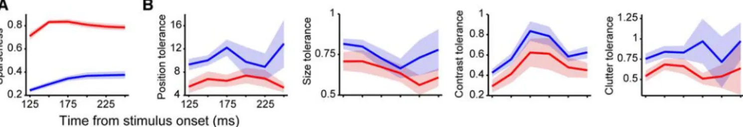
Latency of neuronal responses and time course of selectivity and tolerance properties
We asked whether the subpopulations of weakly and highly se-lective IT neurons show any significant difference in the latency and duration of their responses. In agreement with previous find-ings (Brincat and Connor, 2006), we found a weak but significant positive correlation between object selectivity (i.e., sparseness) and (1) latency of response onset and (2) response duration (see supplemental Table 6A, available at www.jneurosci.org as sup-plemental material). On average, weakly selective neurons fired ⬃10 ms before highly selective cells, and their responses were ⬃30 ms shorter (see supplemental Table 6B, available at www. jneurosci.org as supplemental material). Although the latency of the peak of the response had a tendency to be longer for highly selective neurons than weakly selective neurons, this difference was not significant (see supplemental Table 6B, available at www.jneurosci.org as supplemental material), and no significant correlation was found between peak latency and sparseness (see supplemental Table 6A, available at www.jneurosci.org as sup-plemental material).
Previous studies reported that object selectivity can substan-tially change (e.g., increase) as a function of time during the response epoch (Sugase et al., 1999; Matsumoto et al., 2005; Brin-cat and Connor, 2006). A detailed analysis of the information about object identity conveyed by different temporal epochs of the neuronal response was not the primary goal of this study. However, by measuring the time course of object selectivity as a function of time (using spike count windows of 50 ms that over-lapped of 25 ms) for the two subpopulations of weakly and highly selective neurons defined in Figure 5B, we found that sparseness was remarkably stable for the duration of the IT responses (Fig. 6A). That is, IT neurons that are very object selective in their initial response tend to remain very object selective, and vice versa. A similar analysis of the time course of the tolerance met-rics showed that, despite some modulations as a function of time, highly selective neurons were consistently less tolerant than weakly selective cells for the whole duration of the neuronal re-sponse (Fig. 6B). Overall, these analyses show that selectivity and tolerance metrics are largely independent of the spike count win-Figure 6. Time course of object selectivity (sparseness) and tolerance properties for the two populations of weakly and highly selective neurons.A,B, Sparseness and tolerance properties were computed in spike count windows (time slices) of 50 ms, shifted in steps of 25 ms. In each time slice, the average value (solid line) and the SE (shaded regions) of the sparseness and tolerance properties were computed for the weakly selective neurons (blue;n⫽38) and the highly selective neurons (red;n⫽17) defined in Figure 5 (putative inhibitory neurons were included in the two sets). For each time slice, outliers were removed before averaging (i.e., tolerance metric values larger than 95th percentile in the time slice).
dow (see also supplemental Tables 1, 2, available at www. jneurosci.org as supplemental material) and that the trade-off between selectivity and tolerance holds for the duration of the response.
Relative tolerance of object selectivity
Above, we measured tolerance in absolute terms. Although not the goal of our study, we also collected data that partially address the issue of how well preserved the rank order of object selectivity across different transformations (positions, sizes, and contrasts) is, independent of absolute response rate (i.e., relative tolerance). In particular, for each neuron, we asked how many times the response to the poorly effective object became higher than the response to the effective object, i.e., how many times the object preference of any given neuron reversed over our range of tested identity-preserving transformations (position, size, and con-trast). This was quantified by computing ad⬘index (see Materials and Methods) that measures, for each transformation (e.g., a given position or size), how far apart the responses to the two objects are. A negatived⬘indicates that a given transformation produced a reversal in the object preference of the neuronal re-sponse. Such reversal happened rarely: (1) for position changes, it happened 15% (7%) of the times for the subpopulation of highly (weakly) selective neurons; (2) for size changes, it happened 0% (4%) of the times for the subpopulation of highly (weakly) selec-tive neurons; (3) for contrast changes, the reversal happened 23% (14%) of the times for the subpopulation of highly (weakly) se-lective neurons. Interestingly, even when reversals occurred, they were typically small: the average of the reversedd⬘ for highly selective cells was (1)⫺0.60⫾0.33 (SD) for position changes; and (2)⫺0.64⫾0.50 for contrast changes. The average of the reversedd⬘for weakly selective cells was (1)⫺0.31⫾0.28 for position changes; (2)⫺0.24 ⫾0.17 for size changes; and (3) ⫺0.40⫾0.27 for contrast changes (for comparison, the average d⬘in the reference position was 3.97). This suggests that the re-versal of object preference typically happened when the response to the effective object became as small as the response to the poorly effective object (e.g., at the edges of the receptive fields or for the lowest contrasts), suggesting that the reversal was driven by the variability of two nearly identical neuronal responses, rather than by a true change of object preference. As expected based on our measurements of absolute tolerance (above), such reversals happened more often for the subset of very selective neurons, given the smaller size of their receptive fields and their lower contrast tolerance, compared with the poorly selective cells.
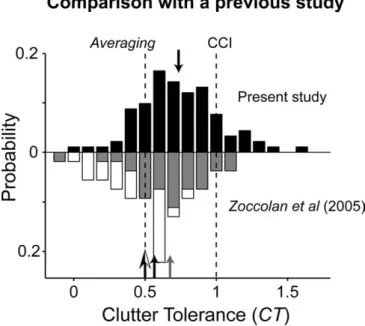
A deeper look into clutter tolerance
Clutter tolerance differs from the other three tolerances tested here because the image changes that one might expect IT neurons to be tolerant to are less well defined. For example, size change has only one degree of freedom, but there is an unlimited number of distractor (clutter) objects that one might add to the visual scene. Considering the overarching goal of the present study (examin-ing the relationship of shape selectivity and tolerance), the most important consideration was to be sure that our choices of flanker (clutter) objects did not produce artifactual dependency between shape selectivity and clutter tolerance.
First, we asked whether the observed strong tendency for weakly shape-selective IT neurons to be less suppressed by flanker objects could be explained by a tendency of those neurons to be more driven by the tested flanker objects when presented in iso-lation. Indeed, this tendency was found in our data (Fig. 7A,
leftmost data points, described further below). However, our clutter tolerance metric (CT; see Materials and Methods) was designed to account for these differences in flanker effectiveness, because the response to the flanker (chosen to be poorly effective in isolation) is subtracted in both the CT numerator and denom-inator (see Materials and Methods). That is, CT is 1.0 whenRref &
flanker⫽Rref(CCI), and CT is 0.5 whenRref & flanker⫽0.5 (Rref⫹
Rflanker) (averaging rule), independent of the effectiveness of the
isolated flanker (Rflanker). To show this lack of bias directly, we
performed Monte Carlo simulations with populations of the same size and response rate distribution as our neuronal data (see Materials and Methods for details). These simulations (Fig. 7B) showed that the observed inverse relationship between sparse-ness and clutter tolerance could not arise (p⬍0.002, one-tailed test) from an implicit correlation between these metrics com-puted over a population of noisy neuronal responses that were all equally tolerant to clutter [i.e., either all completely clutter invari-ant (CCI rule) or all equally suppressed by clutter (averaging rule); see Materials and Methods for details].
Thus, despite possible variations in flanker effectiveness, our CT metric remains unbiased with respect to either a CCI or an averaging rule in clutter. This can be directly appreciated by com-paring the amount of clutter tolerance in the two subpopulations of weakly and highly selective IT neurons (Fig. 5B) as we gradu-ally restricted our analysis to flanker objects with increasingly lower effectiveness (Fig. 7A). As already indicated for our stan-dard analysis (above), flanker objects were, on average, slightly more effective for weakly selective than for highly shape-selective neurons (Fig. 7A, bottom, compare blue and red Figure 7. Additional controls on the relationship between clutter tolerance and object se-lectivity.A, Average CT (top plot) and average effectiveness of the flanker objects relative to the reference objects (bottom plot) for the two subpopulations of weakly (in blue) and highly (in red) shape-selective neurons (as defined in Fig. 5B) as a function of the maximal response evoked by flanker objects (Rflanker) used to compute CT (Rflankerranges from 50 to 5% of the response evoked by the reference object,Rref).Rrefⱖ10 spikes/s for the four leftmost points in the plot. The two rightmost points refer to subsets of neurons with lower (10ⱕRref⬍30 spikes/s) and higher (Rrefⱖ30 spikes/s) effectiveness of the reference object andRflanker⬍ 20%Rref.B, Relationship between sparseness and clutter tolerance obtained from Monte Carlo simulations of two populations of neurons following different clutter rules: CCI and averaging. Each simulation produced a regression line and the regression lines from 500 such simulations are shown in black (CCI) and gray (averaging) in the top panel, together with the regression line through the observed data (dashed). The distributions of correlation coefficients obtained from those simulations are shown at the bottom, together with the correlation coefficient observed in the neuronal data (thick arrow). Two different versions of the averaging rule were imple-mented (see Material and Methods).