Lehigh University
Lehigh Preserve
Theses and Dissertations2013
Online Clinic Appointment Scheduling
Xin Dai
Lehigh University
Follow this and additional works at:http://preserve.lehigh.edu/etd Part of theEngineering Commons
This Thesis is brought to you for free and open access by Lehigh Preserve. It has been accepted for inclusion in Theses and Dissertations by an authorized administrator of Lehigh Preserve. For more information, please [email protected].
Recommended Citation
Online Clinic Appointment Scheduling
by
Xin Dai
A Thesis
Presented to the Graduate and Research Committee
of Lehigh University
in Candidacy for the Degree of
Master of Science
in
Industrial and Systems Engineering
Lehigh University
This thesis is accepted and approved in partial fulfillment of the requirements for the Master of Science. _______________________ Date ______________________ Dr. Robert H. Storer Thesis Advisor ______________________ Dr. Tamás Terlaky Chairperson of Department
iii
Xin Dai Copyright, 2013
ACKNOWLEDGEMENTS
I would like to express my deep gratitude to my thesis adviser, Professor Robert H. Storer, for his patient guidance and valuable suggestions during the development of the thesis.
In addition, I would like to thank my family and friends for their help and constant support.
Content
ACKNOWLEDGEMENT ... iv
LIST OF TABLES ... vii
LIST OF FIGURES ... viii
ABSTRACT ... 1
CHAPTER 1: INTRODUCTION ... 2
1.1. Background ... 2
1.2. Types of Appointment Scheduling ... 2
1.3. Methods of Appointment Scheduling ... 3
1.4. Objectives ... 5
1.5. Outline... 5
CHAPTER 2: LITERATURE REVIEW ... 6
2.1. Overview of Appointment Scheduling ... 6
2.2. Considerations of Appointment Scheduling ... 7
2.3. Measurements of an Appointment System’s Performance ... 11
2.4. Overview of General Papers ... 13
2.5. Review of Related Papers ... 15
CHAPTER 3: PROBLEM STATEMENT ... 19
3.1. Problem Description ... 19
3.3. Proposed Policies ... 21
CHAPTER 4: METHODOLOGIES ... 25
4.1. Problem Definition... 26
4.2. Conceptual Model Formulation ... 26
4.3. Input Data Preparation ... 27
4.4. Output Data Analysis ... 29
CHAPTER 5: RESULTS AND DISCUSSION ... 33
5.1. Preliminary Analysis ... 33
5.2. Simulation Setting ... 34
5.3. Data Analysis and Results Discussion ... 37
Chapter 6: CONCLUSIONS ... 64
6.1. Restatement of Project Objectives ... 64
6.2. Major Findings and Results ... 64
6.3. Future Work ... 67
REFERENCE ... 68
APPENDIX 1: SIMULATION RESULT FOR EACH POLICY ... 74
APPENDIX 2: CONFIDENCE INTERVAL FOR SUGGESTED SOLUTIONS ... 84
List of Tables
Table 5.1 Results of Preliminary Simulation ... 33
Table 5.2: All Scenarios of Analysis ... 36
Table 5.3 Detailed Results of Non-Dominated Solutions for Situation 1... 42
Table 5.4: Detailed Results of Non-Dominated Solutions for Situation 2 ... 49
Table 5.5 Detailed Results of Non-Dominated Solutions for Situation 3... 56
Table 5.6: Detailed Results of Non-Dominated Solutions for Situation 4 ... 63
List of Figures
Figure 5.1 (a): % of Overtime Patients V.S Expected preference for Scenario II in Situation 1 ... 38 Figure 5.1 (b): Expected preference V.S Variance of Preference for Scenario II in Situation 1 ... 38 Figure 5.1 (c): % of Overtime Days V.S % of Overtime Patients for Scenario II in Situation 1 ... 38 Figure 5.2 (a): % of Overtime Patients V.S Expected Preference for Scenario III in Situation 1 ... 39 Figure 5.2 (b): Expected Preference V.S Variance of Preference for Scenario III in Situation 1 ... 40 Figure 5.2 (c): % of Overtime Days V.S % of Overtime Patients for Scenario III in Situation 1 ... 40 Figure 5.3: Non-Dominated Solutions for Situation 1 ... 41 Figure 5.4 (a): % of Overtime Patients V.S Expected Preference for Scenario I in Situation 2 ... 43 Figure 5.4 (b): Expected Preference V.S Variance of Preference for Scenario I in Situation 2 ... 44 Figure 5.4 (c): % of Overtime Days V.S % of Overtime Patients for Scenario I in Situation 2 ... 44
Figure 5.5 (a): % of Overtime Patients V.S Expected Preference for Scenario II in Situation 2 ... 45 Figure 5.5 (b): Expected Preference V.S Variance of Preference for Scenario II in Situation 2 ... 45 Figure 5.5 (c): % of Overtime Days V.S % of Overtime Patients for Scenario II in Situation 2 ... 45 Figure 5.6 (a): % of Overtime Patients V.S Expected Preference for Scenario III in Situation 2 ... 47 Figure 5.6 (b): Expected Preference V.S Variance of Preference for Scenario III in Situation 2 ... 47 Figure 5.6 (c): % of Overtime Days V.S % of Overtime Patients for Scenario III in Situation 2 ... 47 Figure 5.7: Non-Dominated Solutions for Situation 2 ... 49 Figure 5.8 (a): % of Overtime Patients V.S Expected Preference for Scenario I in Situation 3 ... 50 Figure 5.8 (b): Expected Preference V.S Variance of Preference for Scenario I in Situation 3 ... 51 Figure 5.8 (c): % of Overtime Days V.S % of Overtime Patients for Scenario I in Situation 3 ... 51
Figure 5.9 (a): % of Overtime Patients V.S Expected Preference for Scenario II in Situation 2 ... 52 Figure 5.9 (c): % of Overtime Days V.S % of Overtime Patients for Scenario II in Situation 2 ... 52 Figure 5.9 (c): % of Overtime Days V.S % of Overtime Patients for Scenario II in Situation 2 ... 52 Figure 5.10 (a): % of Overtime Patients V.S Expected Preference for Scenario III in Situation 3 ... 54 Figure 5.10 (b): Expected Preference V.S Variance of Preference for Scenario III in Situation 3 ... 54 Figure 5.10 (c): % of Overtime Days V.S % of Overtime Patients for Scenario III in Situation 3 ... 54 Figure 5.11: Non-Dominated Solutions for Situation 3 ... 56 Figure 5.12 (a): % of Overtime Patients V.S Expected Preference for Scenario I in Situation 4 ... 57 Figure 5.12 (b): Expected Preference V.S Variance of Preference for Scenario I in Situation 4 ... 58 Figure 5.12 (c): % of Overtime Days V.S % of Overtime Patients for Scenario I in Situation 4 ... 58
Figure 5.13 (a): % of Overtime Patients V.S Expected Preference for Scenario II in Situation 4 ... 59 Figure 5.13 (b): Expected Preference V.S Variance of Preference for Scenario II in Situation 4 ... 59 Figure 5.13 (c): % of Overtime Days V.S % of Overtime Patients for Scenario II in Situation 4 ... 59 Figure 5.14 a): % of Overtime Patients V.S Expected Preference for Scenario III in Situation 4 ... 61 Figure 5.14 (b): Expected Preference V.S Variance of Preference for Scenario III in Situation 4 ... 61 Figure 5.14 (c): % of Overtime Days V.S % of Overtime Patients for Scenario III in Situation 4 ... 61 Figure 5.15: Non-Dominated Solutions for Situation 4 ... 62 Figure 6.1 All Non-Dominated Solutions for each Request Rate ... 65
ABSTRACT
Health care is a fast growing industry in the United States. Appointment scheduling is one of the key processes in this industry. This thesis focused on on-line appointment system for clinics. The objective of this thesis is to maximize patients’ preferences and the number of patients seen during normal business hours. This is a multi-objective problem to balance the trade-off between overtime and patients’ preferences.
To achieve the objective, a simulation model was built to compare four policies proposed. Emergent patient were always assigned to the same day they requested appointment. In the basic policy, non-emergent patients are assigned to their first preferred date until the reserved capacity for non-emergent patients is full. In Naïve policy,non-emergent patients are always assigned on their first preferred day. Non-emergent patients were assigned based on daily reserved capacity in Policy 1. In Policy 2, it forecasted the expected number of patients to be scheduled for each day and assigned patients to a highly preferred day with lower number of patients scheduled or forecast to be scheduled.
Based on simulation results, it was found that most of non-dominated solutions were close both minimum objective values, so policies proposed were helpful for the clinics to balance overtime and patients’ preferences.
CHAPTER 1: INTRODUCTION
1.1.
Background
Health care is a fast growing industry in the United States. In 2012, total health care expenditures were estimated to be $2.8 trillion and health care spending was about 17.9% of Gross Domestic Product (GDP), which is significantly higher than other developed countries.
Appointment scheduling is one of the key processes in health care industry. A well-designed appointment system can improve patients’ satisfaction and reduce the cost of clinics and hospitals. Outpatient appointment scheduling was first studied by Bailey in the 1950s. This process is most often treated as a queuing system when people study appointment scheduling ( Creemers & Lambrecht, 2009; Cayirli & Veral, 2003).
1.2.
Types of Appointment Scheduling
1.2.1. Traditional Appointment Scheduling
A patient is scheduled for a future appointment time and the number of patient granted an appointment has an upper limit each time period. The appointment lead time could be very long (several weeks or a month in advance), which may result in a high no-show probability.
1.2.2. Open Access Appointment Scheduling
The number of patients request per day is random. A patient is assigned to a time bucket within a relatively short time period (one or two days in advance from the time they request an appointment), since shorter appointment can help to reduce patients’ no-show probability and reduce uncertainty in clinic operations. Robinson and Chen (2009) examined two types of open access scheduling policies. The first policy assumes that all patients are assigned to the same day they request an appointment, and overtime is used to cover excess demand in a time period. The other policy assumes that some patients are assigned to other days if the demand is unusually high. Robinson and Chen also claimed open access scheduling outperforms the traditional appointment scheduling by different performance measurements of appointment system, including over time and idle time of physicians, and patients’ weighted average waiting time. However, this conclusion does not hold when the no-show probability is very small.
1.3.
Methods of Appointment Scheduling
The common methods of requesting an appointment include walk-in, call-in, and online request. When a patient arrives at a clinic or calls the clinic to make an appointment, some clinics will record the appointments by using a scheduling book or a simple online appointment calendar. This is the traditional method to make an
appointment, while online appointment scheduling is more popular nowadays. One Wall Street Journal survey pointed out that the majority of adults prefer the online appointment scheduling. Compared with other methods, the online scheduling system has three advantages: 1) 24-hour convenience: for most clinics, phone access is only available during office hours, while online system is more convenient for patients. 2) time saving: clinic staff spends less time on the phone booking and patients do not need to wait during peak hours in the clinics. 3) patient’s satisfaction: the online scheduling system allows patients to select physicians and time slots based on patients’ preference, which will reduce no-show probability and improve patient health outcomes (Bowser, Utz, Glick, & Harmon, 2010, Schectman, Schorling, & Voss, 2008).
There are two most common types of online scheduling. One is patients input their contact information and type of service requesting through an online request form. The clinic will contact patients and provide an available slot for appointments. Another one is patients can select a physician, type of service requesting and the available appointment slots. The system will automatically confirm the booking without any staff action. In this thesis, the second type of online appointment scheduling is assumed.
1.4.
Objectives
The objectives of this thesis are to propose a policy/ policies to maximize patients’ preferences and the number of patients seen during normal business hours. Thus, this is an multi-objective problem that needs to balance the trade-off between overtime and patients’ preferences.
1.5.
Outline
In this thesis, following this chapter, a literature review will be conducted in Chapter 2. Different ways to define appointment scheduling problem, measurements of appointment system’s performance, and general and related papers will be presented in Chapter 2. The problem definition, assumptions applied in this problem and different policies will be also stated in Chapter 3. Then the method of conducting a simulation model in this thesis will be discussed in Chapter 4. This will be followed by a result analysis and discussion in Chapter 5. At the end of thesis, a conclusion is drawn in Chapter 6.
CHAPTER 2: LITERATURE REVIEW
2.1.
Overview of Appointment Scheduling
Based on the health service required by patients, appointment can be divided into three main categories: primary care clinic, specialty clinic and surgery appointment scheduling (Gupta & Denton, 2008).
2.1.1. Primary Care Clinic Appointment
For primary care practices, the initial care is provided by a single physician or a small group of physicians for families when they faced medical problems. For a multi-physician clinic, when making appointments for patients, patients’ preferred time slots and physicians should be taken into consideration as well as physicians’ availability. The efficiency of clinic and patients’ satisfaction could be improved if a patient can be assigned to a preferred time slot and physician who is familiar with patients’ medical history. Two method of making primary care appointments including advance-schedule, which means patients called a given day before, or, for same-day schedule, which means patients called to schedule an appointment. The number and length of available appointment time slots are various based on the type of service request, medical urgency and providers’ panel (a group of patients that has designated the same provider).
2.1.2. Specialty Care Clinic Appointment
For specialty care clinics, they focus on diagnoses, treatment and recovery for some specialties such as cardiology, neurosurgery and Endocrinology. Some related tests or exams are provided to complete diagnoses or treatments, but they are not achieved by surgical techniques. Sometimes specialists require a referral from a primary care physician or other specialist for patients’ first appointment. The length of available appointment time slots is fixed for most of services. When making appointments for patients, the availability of examination facilities, such as MRI and Scans, should be taken into consideration as well.
2.2.
Considerations of Appointment Scheduling
The goal of appointment scheduling is to provide an optimal policy and achieve a good balance between patients’ satisfaction and the performance of providers or clinics. In the real world, some factors will have influence on the performance of an appointment system, such as punctuality and urgency of patients, no-shows or cancellations, and service process. Thus, when developing a well-designed appointment system, the following main factors should be taken into consideration (Cayirli & Veral, 2003).
2.2.1.
Unpunctuality
Unpunctuality of patients means the difference between patients’ arrival time and actual appointment time. Nuffield Trust studies (1955) implied that more than half of
the patients arrive early, which could cause the congestion of the patient’s waiting room and increase patients’ waiting time. Wijewickrama & Takakuwa (2008) discussed how the impact of no-shows on patients’ waiting time is higher than that of punctuality. Contrary to this result, Blanco White & Pike (1964) showed that the punctuality did not greatly affect performance of appointment systems. In addition, some studies also discussed unpunctuality of physicians as well, in which physicians were late for the first appointment. Vissers (1979) pointed out patients’ waiting time and physicians’ idle time were affected by the unpunctuality of both patients and physicians.
2.2.2. No-shows and Late Cancellations
Some patients are late for their appointments as mentioned in 2.2.2, and some patients miss their appointment as well. This results in a patient no-show problem, which increases underutilization of clinic capacity. Generally, 5-30% is used as a no-show probability in past studies (Ho and Lau, 1992 & 1999; Klassen and Rohleder, 1996; Yang, Lau and Quek, 1998; Cayirli, Veral, and Rosen, 2006 & 2008; Kaandorp and Koole, 2007). Some papers analyzed real data from clinics and pointed out that patients with relatively high no-show probability are younger, male, unmarried, uninsured, with psychosocial problems, of lower socioeconomic status, divorced or widowed and have a history of missed appointments (Neal, Hussain-Gambles, Allgar, Lawlor, and Dempsey, 2005). Daggy et al. (2010) pointed out transportation and appointment lead time affected the no-show probability as well. Similarly, some
papers implied that long appointment lead times increase the no-show rate. Dove and Schneider (1981), Lee et al. (2005) and Gallucci et al. (2005) reported that no-shows were the most influential factor on performance of AS among three environmental factors reviewed (Ho and Lau, 1992). To reduce no-show probability, changing patient behavior or applying overbooking and short lead-time scheduling are suggested (Daggy, etal., 2010).
2.2.3. Preferences of Patients
It has been shown that the accommodation of patients’ preferences can help ensure quality of service provided by primary clinic physicians and increase clinics’ revenues (O’hare and Corlett 2004). The no-show rate can also be reduced if patients’ preferences are matched.
2.2.4. Arrival Characteristics 2.2.4.1. Size of Arrival Units
A single arrival is only one unit, the smallest number handled, that arrive at the system and wait for service, typically a single patient.
A batch arrival is several units entering the system at the same time. In this situation, the time between successive arrivals of the batches may be probabilistic as well as the number of customers in a batch.
2.2.5. Service Characteristics 2.2.5.1. Number of Services
As mentioned before, appointment scheduling is one type of queuing process, so there are two types of queuing stages, including single-stage and multi-stage. Single stage means only one type of service requested when a patient visits the clinic, while multi-stage means a series of branched services may be required in the whole service process. Most papers focus on a single-stage system.
2.2.5.2. Number of Physicians
In queuing theory, queuing systems can be divided into single-server and multiple systems. Physicians are servers in the health care system. In primary care clinics, especially in a multi-physician clinic, physicians have their own panels. Similarly, when scheduling a specialty care clinic and surgery appointments, different physicians are required based on the different services required by patients. In these cases, appointment systems are multi-server systems. When studying the performance of an appointment system, multi-server systems are taken into consideration in some papers such as Wijewickrama & Takakuwa, (2008) and Chao et.al (2003).
2.2.5.3. Service Time
The service time can be random or constant. It can be assumed that the service time of routine appointment at primary care clinic is constant. On the other hand, surgery time is based on the types of surgery and physical conditions of patients, so service time is
randomly distributed. Generally, random service time for surgeries is often modeled by a negative exponential probability distribution (Gross D. and Harris M. ,1985).
2.2.5.4. Queue Discipline
The queue discipline is applied to determine the priority order for patients to be scheduled for an appointment. According to general queuing theory, queue discipline is divided into four main classes, FCFS (first come, first serve), LCFS (last come first served), SIRO (service in random order), and PR (priority ranking). In the appointment scheduling problem, it is assumed that patients are served FCFS in most of papers. In the real world, some clinics apply a priority ranking discipline when they scheduling appointments. For example, clinics give the first priority to emergent patients and second priority to readmission patients. Walk-in patients are usually given to the lowest priority.
2.3.
Measurements of an Appointment System’s Performance
Cayirli and Veral (2003) provided a comprehensive summary of the performance measurement such as patients’ waiting time, providers’ overtime and idle time, and the corresponding cost/penalty.
2.3.1.
Cost-Based
when studies focus on minimizing the cost of appointment cost. In most of cases, costs of patients’ waiting time and physicians’ idle time are the main considerations, such as in Vanden Bosch, Dietz and Simeoni (1999), Lau and Lau (2000), Robinson and Chen (2003).
2.3.2.
Time-Based
Patient’s waiting time and flow time, and physician’s idle time and overtime are measured in terms of mean, maximum, variance and frequency distribution. In general, it is assumed that patient’s waiting time is the difference between the scheduled appointment time and patient’s actual service start time, but waiting time due to early arrival of the patient is not taken into consideration. Patient’ flow time is the total time patient’ spent in the clinic. Physician’s idle time is defined as the waiting time caused by no patients waiting to be seen. Overtime time is the difference between actual and planned finish time of consults. Some papers studied the appointment system problem with time-based measurement, such as O’Keefe (1985), Walter (1973), Vissers and Wijingaard (1979), and Visser, (1979).
2.3.3.
Fairness
Fairness represents the uniformity of performance of an appointment system. It evaluates the mean waiting time of patients according to their place in the queue (Bailey, 1952), variance of waiting time and queue size (Blanco Whit and Pike, 1964, Fetter and Thompson, 1966, Yang, Lau and Quek, 1998).
2.4.
Overview of General Papers
Papers discussing the appointment issue focus on different considerations using different performance measurements. In general, the ways to achieve that could be divided into algorithm development and policy evaluation by simulation tools.
2.4.1.
Algorithm Development
Robinson and Chen (2003) and Mancilla and Storer (2012) focus on algorithm development. Robinson and Chen (2003) tried to balance waiting time and idle time using Monte Carlo integration, solve the problem approximately as a stochastic linear program and develop an atheoretic closed-form heuristic policy. Mancilla and Storer (2012) developed a stochastic scheduling problem considering waiting and idle time and overtime cost for operation room and surgery scheduling. A multi-stage stochastic integer program using sample average approximation was applied to solve this problem.
Erdogan, Denton and Gose (2011) also developed an algorithm to solve dynamic sequencing and scheduling of online appointments to a single stochastic server. The objective was to minimize patient waiting time (indirect and direct) and a clinic’s overtime. In this study, it was assumed that service time and the number of customers to be served are uncertain. A special case of two customers was developed to provide some insights to show tradeoff between the cost of waiting time and likelihood of additional customers arriving. In this special case, the online system scheduled one
customer at a time until the capacity limit was exceeded for a particular day. A two sequencing decisions were assumed. One is first-come- first-served (FCFS). The other one is add-on-first-served (AOFS), in which the second (urgent add-on) customer arrives after the first customer but schedule before the first customer. Two-stage stochastic mixed integer program was proposed to solve the problem. After experimental analysis, they claimed that when all customers have the same cost and service time distribution, FSFC is better than AOFS. If indirect waiting costs are high for add-on customers, they should be scheduled first, otherwise they should be scheduled last.
2.4.2.
Policy Evaluation by Simulation
Daggy et al. (2010) considered a problem that included no show probabilities for each patient the objective is to optimize the number of patients served, the utilization of physicians, and minimizing physician overtime. The patients’ no-show probabilities are estimated by applying a multivariable logistic regression model for each patient. Two policies are used to make a comparison. The one-slot policy is to assign one patient to each time slot without regard to no-show probability. The Mu-Law policy considers different no-show probabilities and assigns a weight to each type of patient. A simulation model was built to compare these policies based on physician utilization and overtime, number of patients served and patient’s waiting time.
appointment overbooking to increase physician productivity and overall clinic performance provide a function a no-show rate and clinic size. Based on simulation results, it turned out overbooking provides more utility when no-show rates are high.
Cayirli et al. (2006) studied the sequence of schedule for the new and returning patients in an ambulatory care system. They considered patient’s waiting time, physician’s idle time and overtime. A simulation model was built in this study to test different sequencing rules and scheduling rules. It was found that sequencing rules have more impact on scheduling rules.
2.5.
Review of Related Papers
The objective of this thesis is to maximize the number of patients seen each day and number of patients assigned to their top preferences. Scheduling of urgent patients is also the consideration in this thesis. Some related papers are reviewed as follows.
Wang and Gupta (2011) considered patients’ preferences and acceptable combinations of physicians and time blocks. They estimated patients’ preferences in terms of acceptance probabilities, which contained difference combinations of date, time and physicians. Second, they assumed an online appointment scheduling system is applied in which patients selected the one preferred date, time blocks and physicians. After receiving the request, the clinic scheduled one combination of date, time and physicians. This decision was made based on 1) patients’ acceptability and arrival
rates at the panel level, 2) average revenue of each appointment, 3) average cost of delaying an advance-book and same day appointment, 4) same-day demand distribution for each physician. If clinic responded that none of the combinations are available, patients can repeat the booking process until they were assigned to an available combination. Two approaches (policies) were presented associated with decision-making. One (H1) is patients are assigned to selected open slots. If more than one time slots are available, the slots with smallest value of appointment slots rank order. Another (H2) is similar with the previous one expect it tries to protect slots for same-day demand by avoiding assigning patients to slots reserved for same-day demand. Compared with the straw policy, they concluded that H1 and H2 can earn more revenue when no-show probability is low.
Feldman et al. (2012) considered an electronic appointment booking systems with patients’ preferences and no-show probability. The objective of this paper was to maximize the expected net “profit” for each day. The profit was the difference between the cost of number of patients that schedule an appointment and show up. They assumed a single physician in the clinic. It was also assumed that one patient can make an appointment on an available day or leave without any appointment if the preferences cannot be met. To estimate the no-show probability, it was assumed that patient choice behavior was followed by multinomial logit choice model. They developed static and dynamic appointment scheduling optimization models to solve the problem. The static model did not consider the state of the booked appointments
and the result pointed out this model is suitable when patient load is high. For dynamic model, it considered the state of booked appointments. An approximate method was proposed by applying a Markov decision process formulation. A simulation study was conducted to compare the four policies. The first and second policy were based on the static and dynamic models respectively. The third policy was a capacity controlled implementation of open access. The last policy was a complement of the third policy offering all days in the scheduling horizon. The criteria were based on expected profit per day and percentage gap between the expected profit per day for the second and other policies. The result pointed out the second policy-dynamic model was a better policy among all policies.
Vermealen et al. (2009) studied an online appointment system considering different urgency of patients and their preferences. This paper considered the situation when a patient made an appointment for a diagnosis test. The objective was to assign patients before their next consult date with the physician. Non-urgent patients were assigned based on minimum access time and urgent patients were assigned to any timeslots left over on days before minimum access time. When considering patients’ preference, three boolean-type preference models were considered work/non-work hours on one day, multiple preferred days and a combination of previous two. Three benchmark policies were proposed to make a selection based on a weighed combination of scheduling performance (capacity utilization) and patients’ preference fulfillment. The first was to assign patients strictly to capacity of urgent/non-urgent patients. The
second was to assign patients to capacity of equal or lower urgency. The last was to assign patients to capacity of equal or lower urgency with dynamic overflow. An experiment was conducted to compare the three policies above. The result showed the trade-off between schedule performance and patients’ preferences.
CHAPTER 3: PROBLEM STATEMENT
3.1.
Problem Description
The problem studied in this thesis is related to online appointment scheduling in a specialist/primary care clinic for both non-emergent patients and emergent patients. Thus, a hybrid approach is considered that accommodates both transitional and open access scheduling. Advance-scheduling is applied to non-emergent patient, while same-day scheduling is allowed for emergent patients. Preference of non-emergent patients’ is a main consideration when the clinic schedules appointments.
3.2.
Problem Assumptions
It is assumed that the daily request rates of all patients followed by a Poisson distribution. The mean request rate of non-emergent patient is 17 per day, while the mean request rate of emergent patient is 3 per day. It is assumed that the total capacity of the clinic is 20 for each day. A certain amount of capacity for emergent patient is reserved, so initially the scheduled capacity of non-emergent patients is 17 and capacity of emergent patients is 3. The clinic assigns patients based on the queuing principle of first come first served and patients’ preference.
assumed that 2-week is the open appointment period here.
For some specialist and primary care clinics, when patients request appointments though an online appointment system, they can choose a combination of preferred dates, time slots and physician. However, in most of clinics, especially in the small clinics, patients cannot choose those in the request form, which will affect patients’ satisfaction. In this thesis, patients are allowed to choose their preferred dates. In addition, since it is assumed that the clinic has multiple undifferentiated physicians and time slots, patients are served by any available physician and time slots. In this case, the preference of physicians and time slots for each patient is not considered, only the day of the appointment. Note that our approach extends to more refined scheduling. For example, instead of daily “time buckets”, our approach would apply to any division of time, for example daily am and pm buckets.
3.3.
Proposed Policies
We propose four different policies for the problem and attempt to balance the trade-off between clinic overtime and meeting patients’ preferences.
3.3.1. Basic Policy
The purpose of this policy is to assign patients based on their preference within limited capacity. This policy is a common policy applied in clinics. Patients can select only one date for each submission in the straw policy, but they can select multiple dates for each submission in the policy described here. In the basic policy, non-emergent patients are assigned to their first preferred date until the reserved capacity for non-emergent patients is full. Emergent patients are assigned on the same-day they requested the appointment. Overtime is allowed for emergent patients. For some patients who cannot be assigned to their most preferred day due to capacity limits of non-emergent patients, the number of already assigned patients for his/her first 5 preferred days will be checked, and he/she will be assigned to the day with the lowest number of assigned patients. The policy ensures that every patient will be assigned with a date, since if all 5 preferred days are over reserved capacity, the patients will still be given an appointment.
3.3.2. Naïve Policy
The purpose of this policy is to maximize patients’ preferences. In this policy, it is an extreme case and assumed the capacity limit is not applied. Thus, non-emergent patients are always assigned on their first preferred day.
3.3.3. Policy 1
The main purpose of this policy is to reduce clinic overtime. A limit of reserved capacity for each day is applied. This daily reserved capacity is fixed for every open appointment period (14 days), but the reserved capacity within these 14 days is different from day to day. For example, the reserved capacity of day 3 for patients requested appointments on day 1 is the same as that of day 4 for patients required appointments on day 2. Generally, the reserved capacity is decreased as we move later in the open appointment period. The way we decide the value of the daily reserved capacity is to calculate the average number of customers who select that day as first five preferences for each day based on multiple replications. For example, day 1-7 is the first open appointment period, and day 2-8 is the second period. For each period, the number of patients that select day 1 as first five preference is 8 and select day 2 as first five preference is 6. So the reserved capacity of first day in each open appointment period is assumed as 14 (if one replication applied).
The detailed procedure for applying this policy is explained as follows.
1. Assign the patients based on their preferences until the daily capacity is reached. That is, clinics assign patients to the most preferred day if the capacity is not exceeded. Otherwise, patients are assigned to the next most preferred day with remaining capacity.
2. If a patient cannot be assigned to his/her first 5 preferences within daily capacity, the procedure will go through his/her first five preferred day and assigned him/ her to a day within the actual capacity of non-emergent patients.
3. If step 2 still fails, the number of already assigned patients for his/her first 5 preferred days will be checked. Then he/she will be assigned to the day with the lowest number of assigned patients.
The purpose of step 2 and 3 is to ensure every patient is assigned and no one is assigned to a day lower than their 5th preferred day.
3.3.4. Policy 2
The purpose of policy 2 is to assign patients to balance patients’ preference and number of patients scheduled for a particular day. The principle of this policy is to forecast the expected number of patients to be scheduled for each day and assign patients to a highly preferred day with lower number of patients scheduled or forecast to be scheduled. The expected number of patients assigned is applied to balance the
patients’ preference and probability of overtime. For each day, the expected number of patients assigned is calculated for the next 14 days (the open appointment period). The way to calculate the expected number of patients is the probability of a day being selected as first preference for each day times the number of patients arriving for each day. The detailed procedure of this process is explained below.
1. Assign the patients based on their preferences until the expected number of patients exceeds capacity. In this case, if the expected number of patients assigned on day3 is 5, but actually 8 patients select day 3 as their first preferred day, then the last 3 patients who request appointments will be assigned to next preferred day if it still has available capacity to assign patients.
2. If a patient cannot be assigned first 5 preferences within the limit, the procedure will go through his/her first five preferred day and assign him/her to a day within the capacity of non-emergent patients.
CHAPTER 4: METHODOLOGIES
Simulation is the key method used to conduct this study. When dealing with complicated models, errors during simulation may occur. Therefore, to reduce these errors, it is necessary to establish a systematic procedure (Banks, 1991) as shown below. Within 11 procedures, the four main elements in a simulation process are selected and presented in detailed in this chapter.
1. Problem definition 2. Project planning 3. System definition
4. Conceptual model formulation 5. Preliminary experimental design 6. Input data preparation
7. Model translation
8. Verification and validation 9. Experimental design
10.Experimentation 11.Output analysis
4.1.
Problem Definition
The purpose of problem definition is to specify the objectives of the project and identify problems which need to be tackled. In addition, it is also helpful when choosing a suitable simulation tool. The objective and problem statement are described in Chapter 1 and 3.
4.2.
Conceptual Model Formulation
This process aims to screen simulation tools and determines the model requirements by comprehending the behavior of the actual system.
At the beginning of the study, the ARENA simulation software was proposed for this study. ARENA has some advantages especially for this study. Firstly, one main function of ARENA is that entities can process through a flow chart of process and seize certain resource as they are processed. It can provide animation when running the program so as-is results (such as current number of patients assigned to each day) can be showed clearly. Secondly, replication parameters (such as replication length, warm-up period and number of replications) can input directly through “Run Setup”. Lastly, a SIMAN summary report (including tally variables, discrete-change variables and counters) can be obtained easily without additional coding input.
However, ARENA’s main function is not to generate random number, although it can do that a few probability distributions. And a lot of “if” loop and “for” loop required for patients’ preference generation and different policy generation, which is not convenient to achieve using ARENA. Therefore, code-based software is preferred and MATLAB was selected for this study. MATLAB is a high-level language and interactive environment for numerical computation, visualization and programming. It allows analyzing data and building models as well. By using MATLAB, the logic of each policy and random number generation are represented easily and clearly. Compared with ARENA, one disadvantage of MATLAB is that extra coding is required for output analysis.
4.3.
Input Data Preparation
Three key input data in the simulation include the number of the two types of patients, who request an appointment each day and the patients’ preference generation. The first two data are discussed in chapter 3 and they can be generated by a simple command in MATLAB. The method for generation of patients’ preference is more complicated and is shown below.
Patients’ preferences are randomly generated as follows. For each patient, his /her preference is an array. The numbers in this array represent the appointment days he/she prefers and the index of the array represents the order of preferred day. For
for this patient is day 3 and second preferred day is day 4 and the third preferred day is day 2.
Based on the description above, the numbers shown in a patient’s preference list should be unique numbers and the value of the number should be less than or equal to 14 due to the 2-week limit of open appointment period in the online system. Firstly, an array (1x1000) of geometric random numbers with probability of 0.2 was generated. However, numbers in this array are not unique numbers nor are they necessarily 14 or less, moving from left to right, duplicated numbers and numbers out of range are removed from this array. Finally, the first 14 elements were selected to represent patients’ preferences. This method generates preferences in such a way that patients prefer days eerily in the 2-week period than later while also including randomness
Based on the method described above, a matrix of patients’ preferences can be generated for all patients requested appointments during the whole simulation horizon.
4.4.
Output Data Analysis
4.4.1. Steady State Simulation
In this stage, adequate information can be obtained through the simulation program with an appropriate model. Types of simulations related to output analysis include terminating simulation and non-terminating (steady state) simulation. Terminating simulation is used for a natural event that specifies the replication length. Initial transient is included in this simulation. Bank operation and military battles are examples of terminating simulation. Steady state simulation is used for no natural event to specify replication length for analyzing the performance of systems in the long run (t∞). In this case, the initial transient should not be taken into consideration for output analysis (Law, 2007). In this thesis, steady state simulation is preferred, since analysis of the systems’ performance after steady state is achieved is main focus for this study. On the other hand, selection of the length of initial transient is important as well. In this simulation model, it is assumed that 280 days are chopped off based on the plot of initial model built and initial transient should be a multiple of the open appointment period. In this case, since the scheduling horizon (the length of replication) is 1000days, the output analysis focused on 720 days which achieves the steady state.
4.4.2. Output Data Analysis - Single Systems
Some results (such as the percentage of overtime days) will be generated for each policy simulation model. However, these results are outcomes of random variables. One important and basic principle of statistics is that every estimate is useless unless accompanied by any measure of accuracy of the estimate. Therefore, more than one replication of the estimate are required and each replication should be independent from each other. In this way, confidence intervals can be obtained to specify estimate accuracy. In addition, if more replications are run, it helps to improve the accuracy of the estimate.
The replications with 95% confidence are applied in the simulation here. The formula used to construct confidence interval:
,where =the mean of
estimate, =0.05, n=20, S= standard deviation of estimate. The formula applied to
standard deviation is
20 1 2 1 i i n X X S .4.4.3. Output Data Analysis - Multiple Systems
Since the initial arrival rate and capacity of non-emergent patients are 17, we would like test the model under different values of arrival rate and capacity. Since four policies are proposed and comparison is needed for analysis to determine which policy is the best policy under each scenario, in this study, the data points are
dependent, but the subjects are independent. To reduce the variance of the estimate comparisons, one variance reduction technique, common random numbers is applied here. In this case, the policies are compared under the same conditions. That is, the number of patients requesting appointments each day and preferences are the same for each policy within one scenario. For example, the number of patients requesting appointments is the same for the first replications of policy 1 and 2, but different for second replications of policy 1 and 2.
Calculation of Output Results
The utilization of the clinic is considered in term of overtime days and number of patients assigned to the overtime period. Expected value and variance of patients’ preferences for the day they are assigned to are used to evaluate how patients’ preferences are met.
a) Percentage of overtime patients
Overtime patients are patients not assigned to normal office hours when the capacity of clinic is exceeded. The percentage of overtime patients is calculated by the total number of overtime patients during the scheduling horizon divided by the total number of patient requests.
b) Percentage of overtime days
Similarly, an overtime day is a day that has some overtime patients. The percentage of overtime days is calculated by the total number of overtime days during the scheduling horizon divided by number of days of the scheduling horizon.
c) Expected value and variance of patients’ preferences
The expected preference refers to the expected value of preference of the day patients are assigned in one scenario. It is calculated by the weighted average of the number of patients assigned to each preferred value. For example, 15 patients are assigned to their first preferred day, 13 patients are assigned to their second preferred day and 12 patients are assigned to their third preferred day. The expected value is 1.925 (1*(15/40) +2*(13/40) +3*(12/40) =1.925).
The variance of preference refers to how far the numbers lie from the expected value of patients’ preferences in one scenario.
CHAPTER 5: RESULTS AND DISCUSSION
5.1.
Preliminary Analysis
A preliminary simulation is conducted to show how patients are assigned under the basic policy. As shown in Table 1, around 30% patients are assigned to their 5th preferred day or worse. Only 34% patients are assigned to their first preferred days and only 63% patients are assigned to their first three preferred days. Apparently, this policy does poorly in meeting most of patients’ satisfaction. To improve this, the tail of the preferred days assigned should be avoided and we must improve portion of patients assigned to their first preferred day or at least first three preferred days. On the other hand, the overtime of the clinic should be taken into consideration as well. Thus, the three policies described in Chapter 3 are proposed on this initiative.
Table 5.1 Results of Preliminary Simulation
Preferred day # of patients assigned % of patients assigned
1st 4193 34% 2nd 2220 18% 3rd 1316 11% 4th 882 7% 5th 663 5% 6th 527 4% 7th 464 4% 8th 404 3% 9th 365 3% 10th 312 3% 11th 280 2% 12th 249 2% 13th 222 2% 14th 183 1%
According to the discussion above, the problem in this thesis is a multi-objective optimization problem which maximizes patients’ preference and minimizes overtime in the clinic. Apparently, none of the policies can achieve the objectives simultaneously, so there is a trade-off between these two aspects and a solution for this type of problem is called non-dominated (Changkong & Haimes, 1983; Hans, 1988). Without any additional information, all non-dominated solutions can be considered candidate solution.
5.2.
Simulation Setting
Three variables will be varied during the simulation, including capacity of non-urgent patient, mean request rate of non-urgent patients, and preference truncation value. To remove the tail of the preferred day assigned, it is preferred to assign patients to their first five preferences if possible, as described in Policy 1 and 2 in Chapter 3.
Therefore, different scenarios are built based on the different values of variables to balance overtime of the clinic and patients’ preferences.
5.2.1. Capacity of Non-Urgent Patients
As mentioned in Chapter 3, it is assumed that a certain amount of capacity is reserved for emergent patients, so the initial reserved capacity for non-emergent patients is 17. During the simulation, the initial reserved capacity will be changed from 15 to 20. In
this case, the capacity reserved for non-emergent patient will be decrease when the value increases.
5.2.2. Patient Request Rate
Initial value of non-emergent patient request rate is 17 per day. The value will be changed from 15 to 18 for different scenarios.
5.2.3. Preference Truncation
As mentioned before, there is a tail of patients who are assigned to the 7th preferred day or worse. To avoid this tail, the performance truncation is set with the range from 1 to 7. For example, if number of preference truncation is 2, this means it is not allowed to assign patients after the second preferred day.
5.2.4. Number of Replications
As mentioned in Chapter 3, multiple replications are required to improve the accuracy of the simulation result. 20 replications are applied in this study to balance accuracy and necessary run time.
5.2.5. Scenario Setting
Based on the setting above, 42 scenarios will be simulated for each mean arrival rate under Policy 1 and Policy 2 respectively, 24 scenarios for each mean arrival rate
under the Basic Policy, and 1 scenario for each mean arrival rate under the Naive Policy. Thus, these scenarios can be categorized and analyzed based on the demand and supply relationship in clinics for each arrival rate: 1) capacity reserved for non-emergent patients is less than the expected value of number of non-emergent patient requests (I), 2) capacity reserved for non-emergent patients is equal to the expected value of number of non-emergent patient requests (II), 3) capacity reserved for non-emergent patients is greater than the expected value of number of non-emergent patient requests (III). Table 5.2 shows the all possible scenarios.
Table 5.2: All Scenarios of Analysis Reserved Capacity of Non-Urgent Patient Request Rate 15 16 17 18 15 II I I I 16 III II I I 17 III III II I
18 III III III II
19 III III III III
5.3.
Data Analysis and Results Discussion
5.3.1. Situation 1: Request Rate=15 5.3.1.1. Analysis of Scenario II
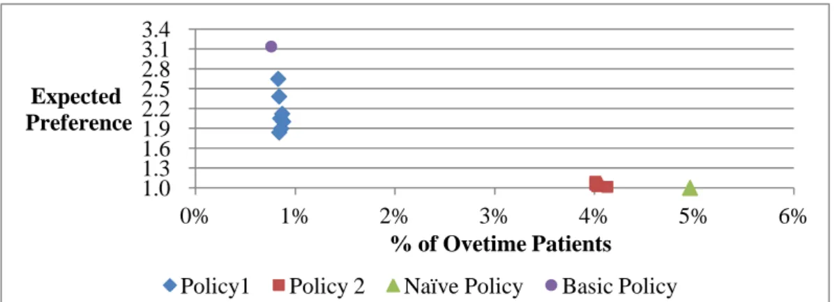
In this scenario, the capacity of non-urgent patients is 15. From figure 5.1 (a), it is clearly shown that both the basic policy and policy 1 have less overtime patients (around 1%) than the naïve policy and policy 2 (greater than 4%). Thus, a similar result can be found in Figure 5.1 (c), which shows the basic policy and policy 1 has less overtime days (less than 10%) than the naïve policy and policy 2 (greater than 25%). In addition, based on Figure 5.1 (a), the expected preferences for the basic policy and policy 1 (greater than 1.8) are higher overtime patients than those values for naïve policy and policy 2 (close to 1). As shown in Figure 5.1 (b), the variance of preference for the basic policy and policy 1 is much higher than the naïve policy and policy 2. For basic policy, the variance of preference is even more than 150, which means patients are assigned to various preferred days and around 13% patients are assigned to their less preferred day, such as 7th preferred day or even the last preferred day (shown in Appendix 1). Thus, according to the analysis above, there is a clear trade-off between patients’ preferences and overtime in clinic. If a clinic would like to satisfy patients’ preference, policy 2 is better than the naïve policy, since the expected preference for policy 2 is very close to 1 and has less overtime patients. If a clinic prefers a less overtime operation, policy 1 is better than the basic policy, since more patients can be assigned to higher preferred days for policy 1.
Figure 5.1 (a): % of Overtime Patients V.S Expected preference for Scenario II in Situation 1
Figure 5.1 (b): Expected preference V.S Variance of Preference for Scenario II in Situation 1
Figure 5.1 (c): % of Overtime Days V.S % of Overtime Patients for Scenario II in Situation 1
*Note: Data points of policy 1 and 2 vary from preference truncation 1 to 7. 1.0 1.3 1.6 1.9 2.2 2.5 2.8 3.1 3.4 0% 1% 2% 3% 4% 5% 6% Expected Preference % of Ovetime Patients
Policy1 Policy 2 Naïve Policy Basic Policy
0 50 100 150 200 1.0 1.5 2.0 2.5 3.0 3.5 Variance of Preference Expected Preference
Policy 1 Policy 2 Naïve Policy Basic Policy
0% 2% 4% 6% 5% 10% 15% 20% 25% 30% % of Overtime Patients % of OT days%
5.3.1.2. Analysis of Scenario III
In this scenario, the reserved capacity of non-urgent patient could be 16,17,18,19 and 20. Similar to scenario II, the naïve policy has the highest value of overtime patients among all policies. In most of cases, policy 1 has less overtime patients than policy 2. Under the similar percentage of overtime patients (as shown in Figure5.2 (a)), the expected value of patients’ preference is lower for the basic policy than the other policies. In addition, unlike the basic policy, the variances of preference for both policy 1 and 2 increases with expect value of preference significantly. The variance of preference decreases with capacity of non-urgent patient and corresponding preference truncation. In Figure 5.2 (c), it can be found that all the cases in policy 2 are within the range of 3%-4% overtime patients and 24%-29% overtime days, while data points are widely spread in policy 1 and basic policy.
Figure 5.2 (a): % of Overtime Patients V.S Expected Preference for Scenario III in Situation 1 0.8 1.1 1.4 1.7 2.0 2.3 0% 1% 2% 3% 4% 5% 6% Expected Preference % of Ovetime Patients
Figure 5.2 (b): Expected Preference V.S Variance of Preference for Scenario III in Situation 1
Figure 5.2 (c): % of Overtime Days V.S % of Overtime Patients for Scenario III in Situation 1
*Note: Data points of policy 1 and 2 vary for preference truncation from 1 to 7 and reserved capacity from 16 to 20 and data points of basic policy vary for reserved capacity from 16 to 20.
5.3.1.3. Summary of Situation 1
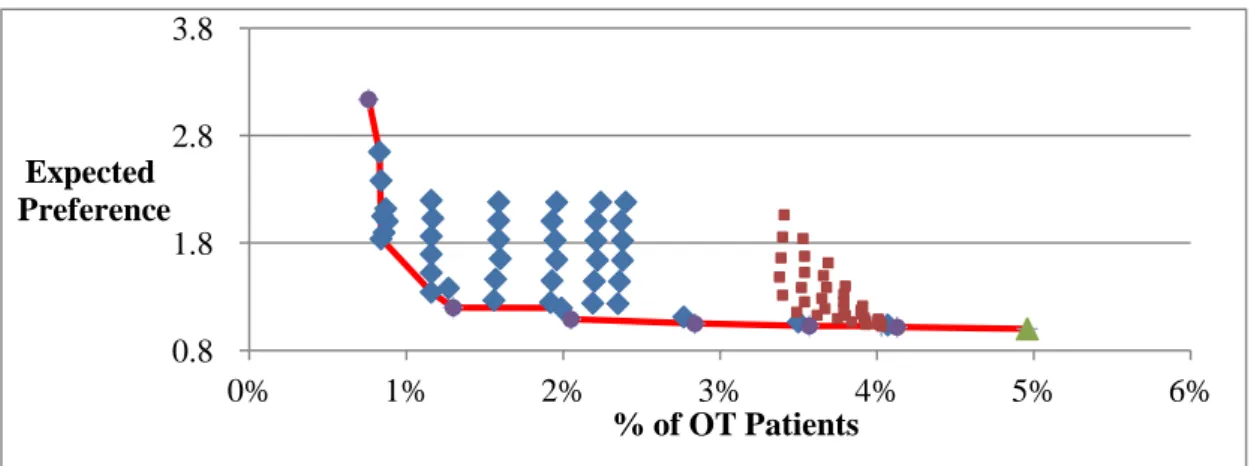
Figure 5.3 shows the non-dominated solutions for situation 1 and detailed results are included in Table 5.3.
In scenario II, after considering the fairness of patients’ assignment, it seems that policy 2 with second preference truncation and naïve policy are equally good due to the similar results of four parameters. Although less overtime operation is required for
0 10 20 30 40 50 1.0 1.2 1.4 1.6 1.8 2.0 2.2 2.4 Variance of Preference Expected Preference
Policy 1 Policy 2 Naïve Policy Basic Policy
0% 2% 4% 6% 5% 10% 15% 20% 25% 30% % of Overtime Patients % of OT days%
policy 1 with second preference truncation, half patients can be assigned to their first preference. Compared with policy 1, 97% patients can be assigned to their first preferred day for policy 2 with second preference truncation and 100% patients can be assigned to their first preferred day for the naïve policy, based on Appendix 1. Thus, if the preference of patients is the main focus, naïve policy and policy 2 with second preference truncation should be selected. If less overtime work is more important, policy 1 with second preference truncation should be selected.
In scenario III, after considering the fairness of patients’ assignment and overtime operation, basic policy when capacity of non-urgent patients is 17 and policy 1 with second preference truncate when capacity of non-urgent patients is 16 are better choices. According to Appendix 1, over 90% of patients are assigned to their first preferred day for basic policy, but only around 70% patients are assigned to their first preferred day for policy 1. Thus, the basic policy is preferred.
Figure 5.3: Non-Dominated Solutions for Situation 1 0.8 1.8 2.8 3.8 0% 1% 2% 3% 4% 5% 6% Expected Preference % of OT Patients
Table 5.3 Detailed Results of Non-Dominated Solutions for Situation 1 Policy Reserved Capacity of Non-Urgent Patient Preference Truncation Request Rate =15 % Overtime Patients Expected Preference Variance of Preference % Overtime Day Naïve policy 4.96% 1 0 27.00% Basic Policy 20 4.13% 1.016 0.096 28.62% Policy 2 15 2 4.03% 1.026 0.159 27.74% Basic Policy 19 3.57% 1.028 0.174 27.61% Basic Policy 18 2.84% 1.049 0.314 24.45% Basic Policy 17 2.05% 1.091 0.611 19.73% Policy 1 17 1 1.99% 1.195 4.108 19.22% Policy 1 16 2 1.16% 1.342 2.985 12.17% Policy 1 15 2 0.84% 1.838 13.947 9.17% Policy 1 15 7 0.83% 2.648 48.155 9.13% Basic Policy 15 0.76% 3.137 151.493 8.53%
5.3.2. Situation 2: Request Rate=16 5.3.2.1. Analysis of Scenario I
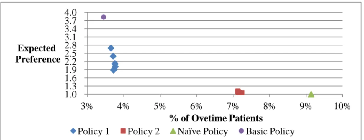
As expected, the naïve policy still has highest percentage of overtime patients in this scenario. As for policy 2, it can meet almost all patients’ preferences, which expected preference is very close to 1.0, although the percentage of overtime patients (5.5%) and number of overtime days (39%) are much higher for policy 1 and the basic policy, even higher than naïve policy (shown in Figure 5.4 (c)). For the basic policy, the percentage of overtime patients is relatively lower, but the expected preference is close to 10 and variance of preference is over 1000, which means a certain number of patients are assigned to 10th preferred day or even worse. Apparently, the basic policy is not a good choice in this scenario. For policy 1, around 2.1% patients are assigned to the overtime period, which is similar to basic policy, but expected preference is approximately to 2.5 when preference truncation is less than 5, which is much better than basic policy.
Figure 5.4 (a): % of Overtime Patients V.S Expected Preference for Scenario I in Situation 2 0.8 1.8 2.8 3.8 4.8 5.8 6.8 7.8 8.8 9.8 10.8 1% 2% 3% 4% 5% 6% 7% 8% Expected Preference % of Ovetime Patients
Figure 5.4 (b): Expected Preference V.S Variance of Preference for Scenario I in Situation 2
Figure 5.4 (c): % of Overtime Days V.S % of Overtime Patients for Scenario I in Situation 2
*Note: Data points of policy 1 and 2 vary for preference truncation from 1 to 7.
5.3.2.2. Analysis of Scenario II
For policy 2 and the naïve policy, the results in this scenario are similar to the results in scenario I. For policy 1, the expected preference is approximately to 2.1 when preference truncation is less than 5 and the percentage of overtime patients and days are around 2.0% and 20% respectively. However, the variance of preference varies based on different values of preference truncation, especially, when preference truncation is greater than 6 in which case the variance of preference is over 30. For
0 200 400 600 800 1,000 1,200 1,400 1.0 3.0 5.0 7.0 9.0 11.0 Variance of Preference Expected Preference
Policy 1 Policy 2 Naïve Policy Basic Policy
0% 2% 4% 6% 8% 15% 20% 25% 30% 35% 40% % of Overtime Patients % of OT days%
the basic policy, the percentage of overtime patients and days are 1.7% and 18.8% respectively, which are the lowest values among all policies, but the expected preference is 3.5 and variance of preference is close to 200 which are the extreme values among all policies as well.
Figure 5.5 (a): % of Overtime Patients V.S Expected Preference for Scenario II in Situation 2
Figure 5.5 (b): Expected Preference V.S Variance of Preference for Scenario II in Situation 2
Figure 5.5 (c): % of Overtime Days V.S % of Overtime Patients for Scenario II in Situation 2 *Note: Data points of policy 1 and 2 vary for preference truncation from 1 to 7.
0.8 1.8 2.8 3.8 2% 3% 4% 5% 6% 7% 8% Expected Preference % of Ovetime Patients
Policy 1 Policy 2 Naïve Policy Basic Policy
0 50 100 150 200 250 1.0 1.5 2.0 2.5 3.0 3.5 4.0 Variance of Preference Expected Preference
Policy 1 Policy 2 Naïve Policy Basic Policy
0% 2% 4% 6% 8% 15% 20% 25% 30% 35% 40% % of Overtime Patients % of OT days%
5.3.2.3. Analysis of Scenario III
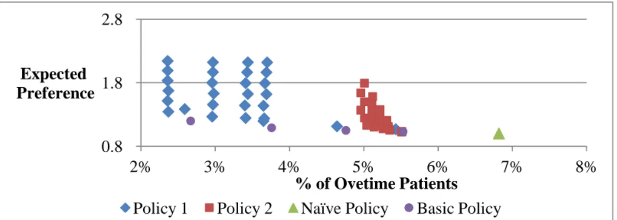
In this scenario, the reserved capacity of non-urgent patient could be 17, 18, 19 and 20. Similar to scenario II, the naïve policy has the highest value of overtime patients among all policies. In most cases, policy 1 has fewer overtime patients than policy 2. Under the similar percentage of overtime patients (as shown in Figure 5.6 (a): the expected value of patients’ preference is lower for basic policy than other policies. In addition, unlike the basic policy, the variance of preference for both policy 1 and 2 increases with expected value of preference significantly. In Figure 5.6 (c), it can be found that all the cases in policy 2 are within the range of 5%-5.5% overtime patients and 36%-39% overtime days, while data points are widely spread in policy 1 and basic policy based on different value set for the reserved capacity of non-urgent patient.
When the capacity of non-urgent patients is 20 and it is preferred to assign patients to their first preferred day for policy 1 and 2, basic policy, policy 1 and policy 2 have the same results, in which expected preference is close to 1.0, the percentage of overtime patients and days are around 5.5% and 38% respectively. In this case, the variance of preference is 0.8 for the basic policy and 1.0 for policy 1 and 2. Thus, these policies satisfy most patients’ preferences, although the percentage of overtime days and patients are relatively high.
Figure 5.6 (a): % of Overtime Patients V.S Expected Preference for Scenario III in Situation 2
Figure 5.6 (b): Expected Preference V.S Variance of Preference for Scenario III in Situation 2
Figure 5.6 (c): % of Overtime Days V.S % of Overtime Patients for Scenario III in Situation 2
*Note: Data points of policy 1 and 2 vary for preference truncation from 1 to 7 and reserved capacity from 17 to 20 and data points of basic policy vary for reserved capacity from 17 to 20. 0.8 1.8 2.8 2% 3% 4% 5% 6% 7% 8% Expected Preference % of Ovetime Patients
Policy 1 Policy 2 Naïve Policy Basic Policy
0 10 20 30 40 1.0 1.2 1.4 1.6 1.8 2.0 2.2 Variance of Preference Expected Preference
Policy 1 Policy 2 Naïve Policy Basic Policy
0% 2% 4% 6% 8% 20% 25% 30% 35% 40% % of Overtime Patients % of OT days%