Holistic Data Cleaning: Putting Violations Into
Context
Xu Chu
1?Ihab F. Ilyas
2Paolo Papotti
21 University of Waterloo, Canada 2 Qatar Computing Research Institute (QCRI), Qatar [email protected], {ikaldas,ppapotti}@qf.org.qa
Abstract—Data cleaning is an important problem and data quality rules are the most promising way to face it with a declarative approach. Previous work has focused on specific formalisms, such as functional dependencies (FDs), conditional functional dependencies (CFDs), and matching dependencies (MDs), and those have always been studied in isolation. Moreover, such techniques are usually applied in a pipeline or interleaved. In this work we tackle the problem in a novel, unified framework. First, we let users specify quality rules using denial constraints with ad-hoc predicates. This language subsumes existing formalisms and can express rules involving numerical values, with predicates such as “greater than” and “less than”. More importantly, we exploit the interaction of the heteroge-neous constraints by encoding them in a conflict hypergraph. Such holistic view of the conflicts is the starting point for a novel definition of repair context which allows us to compute automatically repairs of better quality w.r.t. previous approaches in the literature. Experimental results on real datasets show that the holistic approach outperforms previous algorithms in terms of quality and efficiency of the repair.
I. INTRODUCTION
It is well recognized that business and scientific data are growing exponentially and that they have become a first-class asset for any institution. However, the quality of such data is compromised by sources of noise that are hard to remove in the data life-cycle: imprecision of extractors in computer-assisted data acquisition may lead to missing values, heterogeneity in formats in data integration from multiple sources may introduce duplicate records, and human errors in data entry can violate declared integrity constraints. These issues compromise querying and analysis tasks, with possible damage in billions of dollars [9]. Given the value of clean data for any operation, the ability to improve their quality is a key requirement for effective data management.
Data cleaning refers to the process of detecting and cor-recting errors in data. Various types of data quality rules have been proposed for this goal and great efforts have been made to improve the effectiveness and efficiency of their cleaning algorithms (e.g., [4], [8], [21], [18], [13]). Currently existing techniques are used in isolation. One naive way to enforce all would be to cascade them in a pipeline where different algorithms are used as black boxes to be executed sequentially or in an interleaved way. This approach minimizes the complexity of the problem as it does not consider the
?Work done while interning at QCRI.
interaction between different types of rules. However, this simplification can compromise the quality in the final repair due to the lack of end-to-end quality enforcement mechanism as we show in this paper.
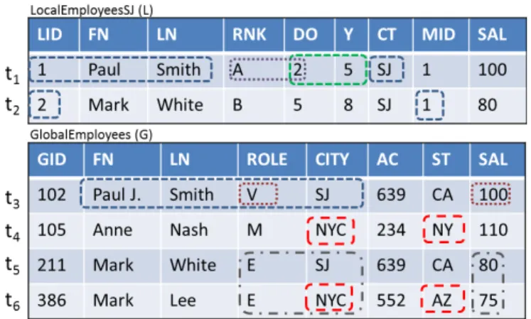
Example 1.1: Consider the GlobalEmployees table (Gfor short) in Figure 1. Every tuple specifies an employee in a company with her id (GID), name (FN, LN), role, city, area code (AC), state (ST), and salary (SAL). We consider only two rules for now. The first is a functional dependency (FD) stating that the city values determine the values for the state attribute. We can see that cells int4 andt6 present a violation for this FD: they have the same value for the city, but different states. We highlight the setS1of four cells involved in the violation in the figure. The second rule states that among employees having the same role, salaries in NYC should be higher. In this case cells int5 andt6 are violating the rule, since employee Lee (in NYC) is earning less than White (in SJ). The set S2 of six cells involved in the violation between Lee and White is also highlighted.
The two rules detect that at least one value in each set of cells is wrong, but taken individually they offer no knowledge of which cells are the erroneous ones.
Fig. 1: Local (L) and Global (G) relations for employees data.
Previously proposed data repairing algorithms focus on re-pairing violations that belong to each class of constraints in isolation, e.g., FD violation repairs [6]. These techniques miss the opportunity of considering the interaction among different classes of constraints violations. For the example above, a
desirable repair would update the city attribute for t6 with a new value, thus only one change in the database would fix the two violations. On the contrary, existing methods would repair the FD by changing one cell inS1, with an equal chance to pick any of the four by being oblivious to violations in other rules. In particular, most algorithms would change the state value for t6 to NY or the state fort4 to AZ. Similarly, rule based approaches, when dealing with application-specific constraints such as the salary constraint above, would change the salaries oft5ort6in order to satisfy the constraints. None of these choices would fix the mistake for city in t6, on the contrary, they would add noise to the existing correct data.
This problem motivates the study of novel methods to correct violations for different types of constrains with de-sirable repairs, where desirability depends on a cost model such as minimizing the number of changes, the number of invented values, or the distance between the value in the original instance and the repair. To this end, we need quality rules that are able to cover existing heterogeneous formalisms and techniques to holistically solve them, while keeping the process automatic and efficient.
Since the focus of this paper is the holistic repair of a set of integrity constraints more general than existing proposals, we introduce a model that accepts as input Denial Constraints (DCs), a declarative specification of the quality rules which generalizes and enlarge the current class of constraints for cleaning data. Cleaning algorithms for DCs have been pro-posed before [4], [20], but they are limited in scope, as they repair numeric values only,generality, only a subclass of DCs is supported, and in thecost model, as they aim at minimizing the distance between original database and repair only. On the contrary, we can repair any value involved in the constraints, we do not have limits on the allowed DCs, and we support multiple quality metrics (including cardinality minimality).
Example 1.2: The two rules described above can be ex-pressed with the following DCs:
c1: ¬(G(g, f, n, r, c, a, s), G(g0, f0, n0, r0, c0, a0, s0),
(c=c0),(s6=s0))
c2: ¬(G(g, f, n, r, c, a, s), G(g0, f0, n0, r0, c0, a0, s0),
(r=r0),(c= “N Y C”),(c06= “N Y C”),(s0 > s))
The DC inc1corresponds to the FD:G.CIT Y →G.ST and has the usual semantics: if two tuples have the same value for city, they must have the same value for state, otherwise there is a violation. The DC in c2 states that every time there are two employees with the same rank, one in NYC and one in a different city, there is a violation if the salary of the second is greater than the salary of the first. Given a set of DCs and a database to be cleaned, our approach starts by compiling the rules into data violations over the instance, so that, by analyzing their interaction, it is possible to identify the cells that are more likely to be wrong. In the example, t6[CIT Y] is involved in both violations, so it is the candidate cell for the repair. Once we have identified what are the cells that are most likely to change, we process their violations to get information about how
to repair them. In the last step, heterogeneous requirements from different constraints are holistically combined in order to fix the violations. In the case of t6[CIT Y], both constraints are satisfied by changing its value to a string different from “NYC”, so we update the cell with a new value.
A. Contributions
We propose a method for the automatic repair of dirty data, by exploiting the evidence collected with the holistic view of the violations:
• We introduce a compilation mechanism to project denial constraints on the current instance and capture the inter-action among constraints as overlaps of the violations on the data instance. We compile violations into a Conflict Hypergraph (CH) which generalizes the one previously used in FD repairing [18] and is the first proposal to treat quality rules with different semantics and numerical operators in a unified artifact.
• We present a novel holistic repairing algorithm that
repair all violations together w.r.t. one unified objective function. The algorithm is independent of the actual cost model and we present heuristics aiming at cardinality and distance minimality.
• We handle different repair semantics by using a novel concept of Repair Context (RC): a set of expressions abstracting the relationship among attribute values and the heterogeneous requirements to repair them. The RC minimizes the number of cells to be looked at, while guaranteeing soundness.
We verify experimentally the effectiveness and scalability of the algorithm. In order to compare with previous approaches, we use both real-life and synthetic datasets. We show that the proposed solution outperforms state of the art algorithms in all scenarios. We also verify that the algorithms scale well with the size of the dataset and the number of quality rules. B. Outline
We discuss related work in Section II, introduce preliminary definitions in Section III, and give an overview of the solution in Section IV. Technical details of the repair algorithms are discussed in Section V. System optimizations are discussed in Section VI, while experiments are reported in Section VII. Finally, conclusions and future work are discussed in Section VIII.
II. RELATEDWORK
In industry, major database vendors have their own products for data quality management, e.g., IBM InfoSphere Quali-tyStage, SAP BusinessObjects, Oracle Enterprise Data Qual-ity, and Google Refine. These systems typically use simple, low-level ETL procedural steps [3]. On the other hand, in academia, researchers are investigating declarative, constraint-based rules [4], [5], [13], [8], [11], [12], [21], [18], which allow users to detect and repair complicated patterns in the
data. However, a unified approach to data cleaning that com-bines evidence from heterogeneous rules is still missing and it is the subject of this work.
Interleaved application of FDs and MDs has been studied before [13] and some works (e.g., [6], [5], [8]) compute sets of cells that are connected by violations from different FDs. This connected component is usually called “equivalence class” and it is a special case of the notion of repair context that we introduce next. Another work [18] exploits the interaction among FDs by using a hypergraph. In our proposal we extend the use of hypergraphs to denial constraints, thus significantly generalizing the original proposal. Moreover, we simplify it, by considering only current violations, thus avoiding a large number of hyperedges that they compute in order to execute the repair process with a single iteration. In fact, by using multiple iterations we can be more general and compute interactions of rules happening in more than two steps.
In this work we compute repairs with a large class of operators in the quality rules: =,6=,<,>,≤,≥,≈(similarity). Most of the previous approaches [6], [8] were dealing only with equality, and can be seen as special cases of our work. Exceptions are [4], [20], where the authors propose algorithms to repair numerical attributes for denial constraints. In our work we extend their results in three important aspects: (i) we treat both strings and numeric values together, thus not restricting updates to numeric values only; (ii) we do not limit the input constraints to local denial constrains; and (iii) we allow multiple quality metrics (including cardinality minimality), while still minimizing the distance between the numeric values in the original and the repaired instances. We show in the experimental study that our algorithms provide repairs of better quality, even for the quality metric in [4].
In general, denial constraints can be extracted from ex-isting business rules with human intervention. Moreover, a source of constraints with numeric values from enterprise databases is data mining [2]. Inferred rules always have a confidence, which clearly points to data quality problems in the instances. For example, a confidence of 98.5% for a rule “discountedPrice<unitPrice” implies that 1.5% of the records require some cleaning.
III. PRELIMINARIES
A. Background
Consider database schema of the formS= (U,R,B), where Uis a set of database domains,Ris a set of database predicates
or relations, andBis a set of finite built-in predicates. In this
paper, B={=, <, >,6=,≤,≈}. For an instance I of S, and
an attributeA∈U, and a tuplet, we denote byDom(A)the
domain of attributeA. We denote byt[A]orI(t[A])the value of the cell of tuplet under attributeA.
In this work we support the subset of integrity con-straints identified by denial constraints (DCs) over relational databases. Denial constraints are first-order formulae of the formϕ:∀x¬(R1(x1)∧. . .∧Rn(xn)∧P1∧. . .∧Pm), where
Ri ∈ R is a relation atom, and x = ∪xi, and each Pi of
the form v1θc, or v1θv2, where v1, v2 ∈ x, c is a constant,
and θ ∈ B. Similarity predicate ≈ is positive when the edit
distance between two strings is above a user-defined threshold
δ.
Single-tuple constraints (such as SQL CHECK constraints), Functional Dependencies, Matching Dependencies, and Con-ditional Functional Dependencies are special cases of unary and binary denial constraints with equality and similarity predicates.
Given a database instanceI of schemaS and a DCϕ, ifI
satisfiesϕ, we writeI|=ϕ. If we have a set of DCΣ,I|= Σ
if and only if∀ϕ∈Σ, I |=ϕ. ArepairI0 of an inconsistent
instance I is an instance that satisfies Σ and has the same set of tuple identifiers in I. Attribute values of tuples in I
andI0 can be different and, for infinite domains of attributes inR, there is an infinite number of possible repairs. Similar to [5], [18], we represent the infinite space of repairs as a finite set of instances with fresh attribute values. In a repair, each fresh valueF V for attributeA can be replaced with a value from Dom(A)\Doma(A), where Doma(A) is the domain
of the values forAwhich satisfy at least a predicate for each denial constraints involvingF V. In other words, fresh values are values of the domain for the actual attributes which do not satisfy any of the predicates defined over them.
Notice that our setting does not rely on restrictions such aslocal constraints[20] or certain regions [14]: it is possible that a repair for a denial constraint triggers a new violation for another constraint. In order to enforce termination of the cleaning algorithm fresh values are introduced in the repair. More details are discussed in the following sections.
B. Problem Definition
Since the number of possible repairs is usually very large and possibly infinite, it is important to define a criterion to identify desirable ones. In fact, we aim at solving the following data cleaning problem: given as input a database I and a set of denial constraints Σ, we compute a repair Ir of I
such that Ir |= Σ (consistency) and their distance cost(Ir,
I) is minimum (accuracy). A popularcost function from the literature [6], [8] is the following:
X
t∈I,t0∈I r,A∈AR
disA(I(t[A]), I(t0[A]))
wheret0 is the repair for tuplet and disA(I(t[A]), I(t0[A]))
is a distance between their values for attribute A (an exact match returns 0)1. There exist many similarity measurements for structured values (such as strings) and our setting does not depend on a particular approach, while for numeric values we rely on the squared Euclidian distance (i.e., the sum of the square of differences). We call this measure of the quality theDistance Cost. It has been shown that finding a repair of minimal cost is NP-complete even for FDs only [6]. Moreover,
1We omit the confidence in the accuracy of attributeAfor tupletbecause it is not available in many practical settings. While our algorithms can support confidence, for simplicity we will consider the cells with confidence value equals to one in the rest of the paper, as confidence does not add specific value to our solution.
minimizing the above function for DCs and numerical values only it is known to be a MaxSNP-hard problem [4].
Interestingly, if we rely on a binary distance between values (0 if they are equal, 1 otherwise), the above cost function corresponds to aiming at computing the repair with the minimal number of changes. The problem of computing such cardinality-minimal repairs is known to be NP-hard to be solved exactly, even in the case with FDs only [18]. We call this quality measure Cardinality-Minimality Cost.
Given the intractability of the problems, our goal is to compute nearly-optimal repairs. We rely on two directions to achieve it: approximation holistic algorithms to identify cells that need to be changed, and local exact algorithms within the cells identified by our notion of Repair Context. We detail our solutions in the following sections.
IV. SOLUTIONOVERVIEW
In this Section, we first present our system architecture, and we explain two data structures: the conflict hypergraph (CH) to encode constraint violations and the repair context (RC) to encode violation repairs.
Fig. 2: Architecture of the system.
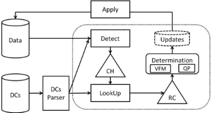
A. System Architecture
The overall system architecture is depicted in Figure 2. Our system takes as input a relational database (Data) and a set of denial constraints (DCs), which express the data quality rules that have to be enforced over the input database.
Example 4.1: Consider the LocalEmployee table (L for short) in Figure 1. Every tuple represents information stored for an employee of the company in one specific location: employee local id (LID), name (FN,LN), rank (RNK), number of days off (DO), number of years in the company (Y), city (CT), manager id (MID), and salary (SAL). LocalEmployee table and GlobalEmployee table constitute the input database. We introduce a third DC:
c3:¬(L(l, f, n, r, d, y, c, m, s), L(l0, f0, n0, r0, d0, y0, c0, m0, s0),
G(g∗, f∗, n∗, r∗, c∗, a∗, s∗),(l6=l0),(l=m0),
(f ≈f∗),(n≈n∗),(c=c∗),(r∗6= “M”))
The constraint states that a manager in the local database L
cannot be listed with a status different from “M” in the global database G. The rule shows how different relations, similarity predicate, and self-joins can be used together.
The DCs Parser provides rules for detecting violations (through the Detect module) and rules for fixing the violations to be executed by the LookUp module as we explain in the following example.
Example 4.2: Given the database in Figure 1, the DCs Parser processes constraintc3and provides the Detect module the rule to identify a violation spanning ten cells over tuples
t1, t2, and t3 as highlighted. Since every cell of this group is a possible error, DCs Parser dictates the LookUp module how to fix the violation if any of the ten cells is considered to be incorrect. For instance, the violation is repaired if “Paul Smith” is not the manager of “Mark White” inL(represented by the repair expression(l6=m0)), if the employee inLdoes not match the one in Gbecause of a different city (c 6=c∗), or if the role for the employee in G is updated to manager
(r∗=M).
We described how each DC is parsed so that violations and fixes for that DC can be obtained. However, our goal is to consider violations from all DCs together and generate fixes holistically. For this goal we introduce two data structures: the Conflict Hypergraph (CH), which encodes all violations into a common graph structure, and the Repair Context (RC), which encodes all necessary information of how to fix violations holistically. The Detect module is responsible for building the CH that is then fed into the LookUp module, which in turn is responsible for building the RC. The RC is finally passed to a Determination procedure to generate updates. Depending on the content of the RC, we have two Determination cores, i.e., Value Frequency Map (VFP) and Quadratic Programming (QP). The updates to the database are applied, and the process is restarted until the database is clean (i.e., empty CH), or a termination condition is met.
B. Violations Representation: Conflict Hypergraph
We represent the violations detected by the Detect module in a graph, where the nodes are the violating cells and the edges link cells involved in the same violation. As an edge can cover more than two nodes, we use a Conflict Hypergraph (CH) [18]. This is an undirected hypergraph with a set of nodes
P representing the cells and a set of annotated hyperedges
E representing the relationships among cells violating a con-straint. More precisely, ahyperedge(c;p1, . . . , pn) is a set of
violating cells such that one of them must change to repair the constraint, and contains: (a) the constraintc, which induced the conflict on the cells; (b) the list of nodesp1, . . . , pn involved
in the conflict.
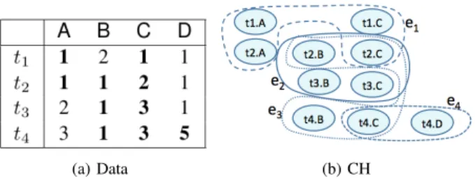
Example 4.3: Consider Relation R in Figure 3a and the following constraints (expressed as FDs and CFDs for read-ability): ϕ1 : A →C,ϕ2 : B →C, and ϕ3 : R[D = 5] →
R[C= 5]. CH is built as in Figure 3b:ϕ1has 1 violation e1;
ϕ2 has 2 violationse2, e3;ϕ3 has 1 violatione4.
The CH represents the current state of the data w.r.t. the constraints. We rely on this representation to analyze the interactions among violations on the actual database. A hyperedge contains only violating cells: in order to repair it,
(a) Data (b) CH
Fig. 3: CH Example.
at least one of its cells must get a new value. Interestingly, we can derive a repair expression for each of the cell involved in a violation, that is, for each variable involved in a predicate of the DC. Given a DC d:∀x¬(P1∧. . .∧Pm)and a set of
violating cells (hyperedge) for it V ={v1, . . . , vn}, for each
vi ∈V there is at least one alternative repair expression of
the formviψt, wheretis a constant or a connected cell inV.
This leads to the following property of hyperedges.
Lemma 4.4: All the repairs for hyperedge ehave at most cardinality nwithn≤m, where mis the size of the biggest chain of connected variables among its repair expressions. Proof Sketch.We start with the case with one predicate only in the DC d. If it involves a constant, then the repair expression contains only one cell and its size coincides with the size of the hyperedge. If it is a predicate involving another cell, then at least one of them is going to change in the repair. We consider now the case with more than a predicate in d. In this case, as the predicates allowed are binary, there may be a chain of connected variables of sizemin the repair expressions: when a value is changed for a cell, it may triggers changes in the connected ones. Therefore, in the worst case, to repair them
m changes are needed. The Lemma states an upper bound for the number of changes that are needed to fix a hyperedge. More importantly, it highlights that in most cases one change suffices as we show in the following example.
Example 4.5: In c3 the biggest chain of variables in the repair expressions comes froml=l0(from the first predicate)
and l 6= m0 (from the second predicate). This means that, to repair violations for c3, at most three changes are needed. Notice that only one change is needed for most of the cells involved in a violation. A na¨ıve approach to the problem is to compute the repair by fixing the hyperedges one after the other in isolation. This would lead to a valid repair, but, if there are interacting violations, it would certainly change more cells than the repair with minimal cost. As our goal is to minimize changes in the repair, we can rely on hyperedges for identifying cells that are very likely to be changed. The intuition here is that, in the spirit of [18], by using algorithms such as the Minimum Vertex Cover (MVC), we can identify at the global level what are the minimum number of violating cells to be changed in
order to compute a repair.2 For instance, a possible MVC for the CH in Figure 3b identifiest2[C]andt4[C].
After detecting all violations in the current database and building the CH, the next step is to generate fixes taking into account the interaction among violations. In order to facilitate a holistic repair, we rely on another data structure, which is discussed next.
C. Fixing Violation Holistically: Repair Context
We start from cells that MVC identifies as likely to be changed, and incrementally identify other cells that are in-volved in the current repair. We call the starting cells and the newly identified onesfrontier. We callrepair expressionsthe list of constant assignments and constraints among the frontier. The frontier and the repair expressions form aRepair Context (RC). We elaborate RC using the following example.
Example 4.6: Consider the database and CH in Example 4.3. Suppose we have t2[C] and t4[C] from the MVC as starting points. We start from t2[C], which is involved in 3 hyperedges. Considere1: givent2[C]to change, the expression
t2[C] =t1[C]must be satisfied to solve it, thus bringingt1[C] into frontier. Cell t1[C] is not involved in other hyperedges, so we stop. Similarly, t2[C] = t3[C] must be satisfied to resolve e2 and t3[C] is brought into the frontier. For e3,
t2[C] = t4[C] is the expression to satisfy, however, t4[C] is involved also in e4. We examine e4 given t4[C] and we get another expressiont4[C] = 5. The resulting RC consists of frontier: t1[C], t2[C], t3[C], t4[C], and repair expressions:
t2[C] =t1[C], t2[C] =t3[C], t2[C] =t4[C], t4[C] = 5. Notice that by starting from t4[C] the same repair is obtained and the frontier contains only four cells instead of ten in the connected component of the hypergraph. An RC is built from a starting cellc with violations from DCsDwith a recursive algorithm (detailed in the next section) and has two properties: (i) there is no cell in its frontier that is not (possibly transitively) connected toc by a predicate in the repair expression of at least ad∈D, (ii) every cell that is (possibly transitively) connected toc by a predicate in the repair expression of at least a d ∈ D is in its frontier. In other terms, RC contains exactly the information required by a repair algorithm to make an informed, holistic decision.
Lemma 4.7: The Repair Context contains the sufficient and necessary information to repair all the cells in its frontier. Proof Sketch.We start with the necessity. By definition, the RC contains the union of the repair expressions over the cells in the frontier. If it is possible to find an assignment that satisfies the repair expressions, all the violations are solved. It is evident that, if we remove one expression, then it is not guaranteed that all violations can be satisfied. The repair expressions are sufficient because of the repair semantics of the DCs. As the frontier contains all the connected cells, any other cell from
V would add an expression that is not needed to repair the violation fordand would require to change a cell that is not needed for the repair. 2In order to keep the execution time acceptable an approximate algorithm is used to compute the MVC.
We can now state the following result regarding the RC: Proposition 4.8: An RC always has a repair of cardinality
n withn≤u, whereuis the size of its frontier. Proof Sketch.From Lemmas 4.7 and 4.4 it can be derived that (i) it is always possible to find a repair for RC, and (ii) in the worst case the repair has the size of the union of the chains of the connected variables in its repair expressions. In practice, the number of cells in a DC is much smaller than the number of cells in the respective hyperedges. For
t6[CIT Y], the size of the RC is one, while there are nine cells in the two hyperedges for c1 andc2.
Given the discussion above, for each cell in the MVC we exploit its violations with the LookUp module to get the RC. Once all the expressions are collected, a Determination step takes as input the RC and computes the valid assignments for the cells involved in it. In this step, we rely on a function to minimize the cost of changing strings (VFM) and on an external Quadratic Programming (QP) tool in order to efficiently solve the system of inequalities that may arise when numeric values are involved. The assignments computed in this step become the updates to the original database in order to fix the violations. The following example illustrates the use of QP, while LookUp and Determination processes will be detailed in the next section.
Example 4.9: Consider again the L relation in Figure 1. Two DCs are defined to check the number of extra days off assigned to each employee:
c4:¬(L(l, f, n, r, d, y, c, m, s),(r= “A”),(d <3)
c5:¬(L(l, f, n, r, d, y, c, m, s),(y >4),(d <4)) In order to minimize the change, the QP formulation of the problem for t1[DO] is (x−2)2 with constraints x ≥3 and
x≥4. Value 4 is returned by QP and assigned tot1[DO]. The holistic reconciliation provided by the RC has several advantages: the cells connected in the RC form a subset of the connected components of the graph and this leads to better efficiency in the computation and better memory management. Moreover, the holistic choice done in the RC minimizes the number of changes for the same cell; instead of trying different possible repairs, an informed choice is made by considering all the constraints on the connected cells. We will see how this leads to better repairs w.r.t. previous approaches.
V. COMPUTINGTHEREPAIRS
In this Section we give the details of our algorithms. We start by presenting the iterative algorithm that coordinates the detect and repair processes. We then detail the technical solu-tions we built for DETECT, LOOKUP, and DETERMINATION. A. Iterative Algorithm
Given a database and a set of DCs, we rely on Algorithm 1. It starts by computing violations, the CH, and the MVC over it. These steps bootstrap the outer loop (lines 5–26), which is repeated until the current database is clean (lines 19–22) or a termination condition is met (lines 23–26). Cells in the MVC are ranked in order to favor those involved in more violations
Algorithm 1 Holistic Repair
Input: Database data, Denial Constraints dcs Output: Repair data
1: Compute violations, conflict hypergraph, MVC.
2: Let processedCells be a set of cells in the database that have already been processed.
3: sizeBefore←0 4: sizeAfter←0 5: repeat
6: sizeBefore← processedCell.size()
7: mvc ← Re-order the vertices in MVC in a priority queue according to the number of hyperedges
8: while mvc is not emptydo
9: cell←Get one cell from mvc
10: rc←Initialize a new repair context for that cell
11: edges← Get all hyperedges for that cell
12: whileedges is not empty do
13: edge← Get an edge from edges
14: LOOKUP(cell, edge, rc) 15: end while
16: assignments← DETERMINATION(cell, exps) 17: data.update(assignments)
18: end while
19: reset the graph: re-build hyperedges, get new MVC
20: if graph has no edgesthen
21: return data
22: end if
23: tempCells←graph.getAllCellsInAllEdges() 24: processedCells←processedCells∪tempCells
25: sizeAfter←processedCell.size() 26: untilsizeBefore ≤sizeAfter
27: return data.P ostP rocess(tempCells, M V C)
and are repaired in the inner loop (lines 8–18). In this loop, the RC for the cell is created with the LOOKUP procedure. When the RC is completed, the DETERMINATIONstep assigns the values to the cells that have a constant assignments in the repair expressions (e.g., t1[A] = 5). Cells that do not have assignments with constants (e.g.,t1[A]6= 1), keep their value and their repair is delayed to the next outer loop iteration. If the updates lead to a new database without violations, then it can be returned as a repair, otherwise the outer loop is executed again. If no new cells have been involved w.r.t. the previous loop, then the termination condition is triggered and the cells without assignments are updated with new fresh values in the post processing final step.
The outer loop has a key role in the repair. In fact, it is possible that an assignment computed in the determination step solves a violation, but raises a new one with values that were not involved in the original CH. This new violation is identified at the end of the inner loop and a new version of the CH is created. This CH has new cells involved in violations and therefore the termination condition is not met.
all the cells in the last MVC (computed at line 19) to fresh values. This guarantees the consistency of the repair and no new violations can be triggered. Pushing to the very last the assignment of a fresh value forces the outer loop to try to find a repair with constants until the termination condition is met, as we illustrate in the following example.
Example 5.1: Consider again only rules c1 and c2 in the running example. After the first inner loop iteration, the RC contains an assignment t6[CITY] 6= “N Y C”, which is not enforced by the determination step and therefore the database does not change. The HC is created again (line 19) and it still has violations for c1 and c2. The cells involved in the two violations go into tempCells andsizeAfter is set to 9. A new outer loop iteration sets sizeBeforeto 9, the inner loop does not change the data, and it gets again the same graph at line 19. As sizeBefore = sizeAfter, it exits the outer loop and the post processing assigns t6[CITY] = “F V”. Proposition 5.2: For every set of DCs, if the determination step is polynomial, thenHolistic Repairis a polynomial time algorithm for the data cleaning problem. Proof sketch.It is easy to see that the output of the algorithm is a repair for an input databaseD with DCsdcs. In the outer loop we change cells to constants that satisfy the violations and in the post process we resolve violations that were not fixable with a constant by introducing fresh values. As fresh values do not match any predicate, the process eventually terminates and returns a repair which does not violate the DCs anymore. The vertex cover problem is an NP-complete problem and there are standard approaches to find approximate solutions. We use a greedy algorithm with factorkapproximation, where
k is the maximum number of cells in a hyperedge of the HC. Our experimental studies show that a k approximation of the MVC lead to better results w.r.t. alternative ways to identify the seed cells for the algorithm. The complexity of the greedy algorithm is linear in the number of edges. In the worst case, the number of iterations of the outer loop is bounded by the number of constraints in dcplus one: it is possible to design a set of DCs that trigger a new violation at each repair, plus one extra iteration to verify the termination condition. The complexity of the algorithm is bounded by the polynomial time for the detection step: three atoms in the DC need a cubic number of comparisons in order to check all the possible triplets of tuples in the database. In practice, the number of tuples is orders of magnitude bigger than the number of DCs and therefore the size of the data dominates the complexity
O(|data|c|dcs|), wherec is the largest number of atoms in a
rule ofdcs. The complexity of the inner loop depends on the number of edges in the CH and on the complexity of LOOKUP
and DETERMINATIONthat we discuss next. Though Algorithm 1 is sound, it is not optimal, as it is illustrated in the following example.
Example 5.3: Consider again Example 4.3. We showed a repair with four changes obtained with our algorithm, but there exists a cardinality minimal repair with only three changes:
t1[C] = 3, t2[C] = 3, t4[D] =N V. We now describe the functions to generate and manipulate the
predicate in dcs = 6= > >= < <= ≈t
predicate in repair exps 6= = <= < >= > 6=t
TABLE I: Table of conversion of the predicates in a DC for their repair. Predicate6=tstates that the distance between two
strings must be greater thant.
building blocks of our approach. B. DETECT: Identifying Violations
Identifying violations is straightforward: every valid assign-ment for the denial constraint is tested, if all the atoms for an assignment are satisfied, then there is a violation.
However, the detection step is the most expensive operation in the approach as the complexity is polynomial with the number of atoms in the DC as the exponent. For example, in the case of simple pairwise comparisons (such as in FDs), the complexity is quadratic in the number of tuples, and it is cubic for constraints such as c3 in Example 4.1. This is also exacerbated by the case of similarity comparisons, when, instead of equality check, there is the need to compute edit distances between strings, which is an expensive operation.
In order to improve the execution time on large relations, optimization techniques for matching records [10] are used. In particular, the blocking method partitions the relations into blocks based on discriminating attributes (or blocking keys), such that only tuples in the same block are compared. C. LOOKUP: Building the Repair Context
Given a hyperedge e = {c;p1, . . . , pn} and a cell p =
ti[Aj] ∈P, the repair expression r for pmay involve other
cells that need to be taken into account when assigning a value top. In particular, giveneandp, we can define a rule for the generation of repair expressions.
Asp∈Aφ(c), then it is required thatr:pφcc, whereφc is
the predicate converted as described in Table I. Variableccan be a constant or another cell. For denial constraints, we defined a function DC.Repair(e,c), based on the above rule, which automatically generates a repair expression for a hyperedgee
and a cell c. We first show an example of its output when constants are involved in the predicate and then we discuss the case with variables.
Example 5.4: Consider the constraintc2from the example in Figure 1. We show below two examples of repair expres-sions for it.
DC.Repair((c2;t5[ROLE], t5[CITY], t5[SAL], . . . , t6[SAL]),
t5[ROLE]) ={t5[ROLE]6= “E”} DC.Repair((c2;t5[ROLE], t5[CITY], t5[SAL], . . . , t6[SAL]),
t6[SAL]) ={t6[SAL]≥80} In the first repair expression the new value for t5[ROLE] must be different from “E” to solve the violation. The re-pair expression does not state that its new value should be different from the active domain of ROLE (i.e., t5[ROLE] 6= {“E”,“S”,“M”}), because in the next iteration of the outer loop it is possible that another repair expression imposes
t5[ROLE]to be equal to a constant already in the active domain (e.g., a MD used for entity resolution). If there is no other expression suggesting values fort5[ROLE], in a following step the termination condition will be reached and the post-process will assign a fresh value to t5[ROLE]. Given a cell to be repaired, every time another variable is involved in a predicate, at least another cell is involved in the determination of its new value. As these cells must be taken into account, we also collect their expressions, thus possibly triggering the inclusion of new cells. We call LOOKUP the recursive exploration of the cells involved in a decision. Algorithm 2 LOOKUP
Input: Cell cell, Hyperedge edge, Repair Context rc Output: updated rc
1: exps←Denial.repair(edge, cell) 2: frontier←exps.getF rontier() 3: for allcell∈frontierdo
4: edges←cell.getEdges() 5: for alledge ∈edgesdo
6: exps←exps ∪LOOKUP(cell,edge,rc).getExps() 7: end for
8: end for
9: rc.update(exps)
Algorithm 2 describes how, given a cellc and a hyperedge
e, LOOKUP processes recursively in order to move from a single repair expression for c to aRepair Context.
Proposition 5.5: For every set of DCs and cellc,LOOKUP
always terminates in linear time and returns a Repair Context
for c.
Proof sketch. The correctness of the RC follows from the traversal of the entire graph. Cycles are avoided as in the expressions the algorithm keeps track of previously visited nodes. As it is a Depth-first search, its complexity is linear in the size of graph and is O(2V −1), where V is the largest number of connected cells in an RC. Example 5.6: Consider the constraintc3 from the example in Figure 1 and the DC:
c6:¬(G(g, f, n, r, c, a, s),(r= “V”),(s <200)) That is, a vice-president cannot earn less than 200. Given
t3[ROLE] as input, LOOKUP processes the two edges over it and collects the repair expressions t3[ROLE]6= “V” from c6 andt3[ROLE] = “M” fromc3.
D. DETERMINATION: Finding Valid Assignments
Given the set of repair expressions collected in the RC, the DETERMINATION function returns an assignment for the frontier in the RC. The process for the determination is depicted in Algorithm 3: Given an RC and a starting cell, we first choose a (maximal) subset of the repair expressions that is satisfiable, then we compute the value for the cells in the frontier aiming at minimizing the cost function, and update the database accordingly later.
Algorithm 3 DETERMINATION
Input: Cell cell, Repair Context rc Output: Assignments assigns
1: exps ←rc.getExps()
2: if exps contain >, <, >=, <=then
3: QP ←computeSatisfiable(exps) 4: assigns ←QP.getAssigments() 5: else 6: V F M ← computeSatisfiable(exps) 7: assigns ←V F M.getAssigments() 8: end if 9: return assigns
In Algorithm 3, we have two determination procedures. One is Value Frequency Map (VFM), which deals with string typed expressions. The other is quadratic programming (QP), which deals with numerical typed expressions3.
1) Function computeSatisfiable: Given the current set of expressions in the context, this function identifies the subset of expressions that are solvable.
Some edges may be needed to be removed from the RC to make it solvable. First, a satisfiability test verifies if the repair expressions are in contradiction. If the set is not satisfiable, the repair expressions coming from the hyperedge with the smallest number of cells are removed. If the set of expressions is now satisfiable, the removed hyperedge is pushed to the outer loop in the main algorithm for repair. Otherwise, the original set minus the next hyperedge is tested. The process of excluding hyperedges is then repeated for pairs, triples, and so on, until a satisfiable set of expressions is identified. In the worst case, the function is exponential in the number of edges in the current repair context. The following example illustrates how the function works.
Example 5.7: Consider the example in Figure 1 and two new DCs:
c7: ¬(L(l, f, n, r, d, y, c, m, s),(r= “B”),(d >4))
c8: ¬(L(l, f, n, r, d, y, c, m, s),(y >7),(d <6)) That is, an employee after 8 years should have at least 6 extra days off, and an employee of rank “B” cannot have more than 4 days. Given t2[DO] as input by the MVC, LOOKUP processes the two edges over it and collects the repair expressions t2[DO]≤4 from c7 andt2[DO]≥6 from
c8. The satisfiability test fails (x ≤ 4 ∧x ≥ 6) and the computeSatisfiablefunction starts removing expressions from the RC, in order to maximize the set of satisfiable constraints. In this case, it removesc7 from the RC and sets t2[DO] = 6 to satisfyc8. Violation forc7is pushed to the outer loop, and, as in the new MVC there are no new cells involved, the post processing step updatest2[RNK]to a fresh value. 2) Function getAssignments: After getting the maximum number of solvable expressions, the following step aims at computing an optimal repair according to the cost model at
hand. We therefore distinguish between string typed expres-sions and numerical typed expresexpres-sions for both cost models: cardinality minimality and distance minimality
String Cardinality Minimality. In this case we want to minimize the number of cells to change. For string type, expressions consist only of=and6=, thus we create a mapping from each candidate value to the occurrence frequency (VFM). The value with biggest frequency count will be chosen.
Example 5.8: Consider a schema R(A, B) with 5 tu-ples t1 = R(a, b), t2 = R(a, b), t3 = R(a, cde), t4 =
R(a, cdf), t5 = R(a, cdg). R has an F D : A → B. Suppose now we have an RC with set of expressionst1[B] =
t2[B] = t3[B] = t4[B] = t5[B]. VFM is created with
b → 2, cde → 1, cdf → 1, cdg → 1. So value b is chosen.
String Distance Minimality. In this case we want to minimize the string edit distance. Thus we need a different VFM, which maps from each candidate value to the edit distance if this value were to be chosen.
Example 5.9: Consider the same database as Example 5.8. String cardinality minimality is not necessarily string distance minimality. Now VFM is created as follows: b →12, cde→
10, cdf → 10, cdg → 10. So any of cde, cdf, cdg can be
chosen.
Numerical Distance Minimality. In this case we want to minimize the squared distance. QP is our determination core. In particular, we need to solve the following objective function: for each cell with value v involved in a predicate of the DC, a variable x is added to the function with (x−v)2. The expressions in the RC are transformed into constraints for the problem by using the same variable of the function. As the objective function given as a quadratic has a positive definite matrix, the quadratic program is efficiently solvable [19].
Example 5.10: Consider a schemaR(A, B, C)with a tuple
t1 =R(0,3,2) and the two repair expressions: r1 : R[A]<
R[B] and r2 : R[B] < R[C]. To find valid assignments, we want to minimize the quadratic objective function (x−0)2+ (y−3)2+(z−2)2with two linear constraintsx < yandy < z, where x, y, z will be new values for t1[A], t1[B], t1[C]. We get solution x= 1, y= 2, z= 3 with the value of objective
function being 3.
Numerical Cardinality Minimality. In this case we want (i) to minimize the number of changed cells, and (ii) to minimize the distance for those changing cells. In order to achieve cardinality minimality for numerical values, we gradually increase the number of cells that can be changed until QP becomes solvable. For those variables we decide not to change, we add constraint to enforce it to be equal to original values. It can be seen that this process is exponential in the number of cells in the RC.
Example 5.11: Consider the same database as in Example 5.10.Numerical distance minimality is not necessary numerical cardinality minimum. It can be easily spotted that x= 0, y= 1, z = 2 whose squared distance is 4 only has one change, while x = 1, y = 2, z = 3 whose squared is 3 has three
changes.
VI. OPTIMIZATIONS ANDEXTENSIONS
In this section, we briefly discuss two optimization tech-niques adopted in our system, followed by two possible exten-sions that may be of interest to certain application scenarios. Detection Optimization. Violation detection for DCs checks every possible grounding of predicates in denial con-straints. Thus improving the execution times for violation detection implies reducing the number of groundings to be checked. We face the issue by verifying predicates in a order based on their selectivity. Before enumerating all grounding combinations, predicates with constants are applied first to rule out impossible groundings. Then, if there is an equality pred-icate without constants, the database is partitioned according to two attributes in the equality predicate, so that grounding from two different partitions need not to be checked. Consider for examplec3. The predicate (r∗ 6= ‘M0) is applied first to rule out grounding with attributer∗equalsM. Then predicate
(l = m0) is chosen to partition the database, so groundings with values of attributes l and m0 not being in the same
partition will not be checked.
Hypergraph Compression. The conflict hypergraph pro-vides a violation representation mechanism, such that all information necessary for repairing can be collected by the LOOKUP module. Thus, the size of the hypergraph has an impact on the execution time of the algorithm. We therefore reduce the number of hyperedges without compromising the repair context by removing redundant edges. Consider for example a table T(A, B) with 3 tuples t1 = (a1, b1), t2 = (a1, b2), t3 = (a1, b3) and an FD: A → B; it has three hyperedges and three expressions in the repair context, i.e.,
t1[B] = t2[B], t1[B] = t3[B], t2[B] = t3[B]. However, only two of them are necessary, because the expression for the third hyperedge can be deduced from the first two.
Custom Repair Strategy. The default repair strategy can easily be personalized with a user interface for the LOOKUP
module. For example, if a user wants to enforce the increase of the salary for the NYC employee in rule c2, she just needs to select the s variable in the rule. An alternative representation of the rule can be provided by sampling the rule with an instance on the actual data, for example ¬(G(386, M ark, Lee, E, N Y C,552, AZ,75),G(M ark, W hite, E, SJ,639, CA,80),(80 > 75)), and the user high-lights the value to be changed in order to repair the violation. We have shown how repair expressions can be obtained automatically for DCs. In general, theRepairfunction can be provided for any new kind of constraints that is plugged to the system. In case the function is not provided, the system would only detect violating cells with the Detect module. The iterative algorithm will try to fix the violation with repair expressions from other interacting constraints or, if it is not possible, it will delay its repair until the post-processing step. Manual Determination.In certain applications, users may want to manually assign values to dirty cells. In general, if a user wants to verify the value proposed by the system for a repair, and eventually change it, she needs to analyze what are
the cells involved in a violation. In this scenario, the RC can expose exactly the cells that need to be evaluated by the user in the manual determination. Even more importantly, the RC contains all the information (such as constants assignments and expressions over variables) that lead to the repair. In the same fashion, fresh values added in the post processing step can be exposed to the user with their RC for examination and manual determination.
VII. EXPERIMENTALSTUDY
The techniques have been implemented as part of the
NADEEF data cleaning project at QCRI4 and we now present
experiments to show their performance. We used real-world and synthetic data to evaluate our solution compared to state-of-the-art approaches in terms of both effectiveness and scalability.
A. Experimental Settings
Datasets. In order to compare our solution to other ap-proaches we selected three datasets.
The first one, HOSP, is from US Department of Health & Human Services [1].HOSPhas 100K tuples with 19 attributes and we designed 9 FDs for it. The second one, CLIENT [4], has 100K tuples, 6 attributes over 2 relations, and 2 DCs involving numerical values. The third one, EMP, contains synthetic data and follows the structure of the running example depicted in Figure 1. We generated up to 100K tuples for the 17 attributes over 2 relations. The DCs are c1, . . . , c6 as presented in the paper.
Errors in the datasets have been produced by introducing noise with a certain rate, that is, the ratio of the number of dirty cells to the total number of cells in the dataset. An error rate e% indicates that for each cell, there is ae%probability we are going to change that cell. In particular, we update the cells containing strings by randomly picking a character in the string, and change it to “X”, while cells with numerical values are updated with randomly changing a value from an interval.5 Algorithms. The techniques presented in the paper have been implemented in Java. As our holistic Algorithm 1 is modular with respect to the cost function that the user wants to minimize, we implemented the two semantics discussed in Section V-D. In particular we tested the getAssigment function both for cardinality minimality (RC-C) and for the minimization of the distance (RC-D).
We implemented also the following algorithms in Java: the FD repair algorithms from [5] (Sample), [6] (Greedy), [18] (VC) forHOSP; and the DC repair algorithm from [4] (MWSC) for CLIENT. As there is no available algorithm able to repair all the DCs in EMP, we compare our approach against a sequence of applications of other algorithms (Sequence). In particular, we ran a combination of three algorithms: Greedy for DCs c1, MWSC for c2, c4, c5, c6, and a simple, ad-hoc algorithm to repair c3 as it is not supported by any of the existing algorithms. In particular, for c3 we implemented a
4http://da.qcri.org/NADEEF/
5Datasets can be downloaded at http://da.qcri.org/hc/data.zip
simplified version of our Algorithm 1, without MVC and with violations fixed one after the other without looking at their interactions. As there are six alternative orderings, we executed all of them for each test and picked the results from the combination with the best performance. For ≈t we used
string edit distance with t = 3: two strings were considered similar if the minimum number of single-character insertions, deletions and substitutions needed to convert a string into the other was smaller than 4.
Metrics. We measure performance with different metrics, depending on the constraints involved in the scenario and on the cost model at hand. The number of changes in the repair is the most natural measure for cardinality minimality, while we use the cost function in Section III-B to measure the distance between the original instance and its repair. Moreover, as the ground truth for these datasets is available, to get a better insight about repair quality we measured also precision (P, corrected changes in the repair), recall (R, coverage of the errors introduced with e%), and F-measure (F = 2×(P ×
R) (P+R)). Finally, we measure the execution times needed to obtain a repair.
As in [5], we count as correct changes the values in the repair that coincide with the values in the ground truth, but we count as a fraction (0.5) the number of partially correct changes: changes in the repair which fix dirty values, but their updates do not reflect the values in the ground truth. It is evident that fresh values will always be part of the partially correct changes.
All experiments were conducted on a Win7 machine with a 3.4GHz Intel CPU and 4GB of RAM. Gurobi Optimizer 5.0 has been used as the external QP tool [16] and all computations were executed in memory. Each experiment was run 6 times, and the results for the best execution are reported. We decided to pick the best results instead of the average in order to favor Sample, which is based on a sampling of the possible repairs and has no guarantee that the best repair is computed first. B. Experimental Results
We start by discussing repair quality and scalability for each dataset. Depending on the constraints in the dataset, we were able to use at least two alternative approaches. We then show how the algorithms can handle a large number of constraints holistically. Finally, we show the impact of the MVC on our repairs.
Exp-1: FDs only. In the first set of experiments we show that the holistic approach has benefits even when the con-straints are all of the same kind, in this case FDs. As in this example all the alternative approaches consider some kind of cardinality minimality as a goal, we ran our algorithm with the getAssigmentfunction set for cardinality minimality (RC-C).
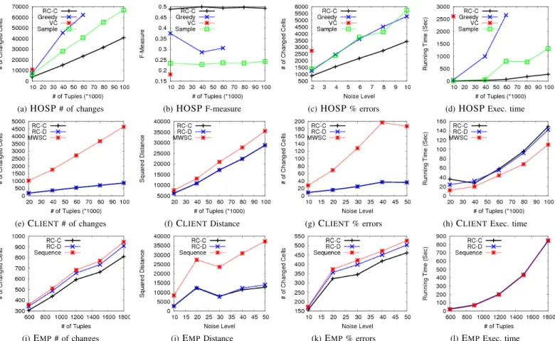
Figures 4(a-c) report results on the quality of the repairs generated for the HOSP data with four systems. Our system clearly outperforms all alternatives in every quality measure. This verifies that holistic repairs are more accurate than alter-native fixes. The low values for the F-measure are expected: even if the precision is very high (about 0.9 for our approach
(a)HOSP# of changes (b)HOSPF-measure (c)HOSP% errors (d)HOSPExec. time
(e)CLIENT# of changes (f)CLIENTDistance (g)CLIENT% errors (h)CLIENTExec. time
(i)EMP# of changes (j)EMPDistance (k)EMP% errors (l)EMPExec. time
Fig. 4: Experimental results for the data cleaning problem.
on 5% error rate), recall is always low because many randomly introduced error cannot be detected. Consider for example R(A,B), with an FD: A→B, and two tuples R(1,2), R(1,3). An error introduced for a value in A does not trigger a violation, as there is not match in the left hand side of the FD, thus the erroneous value cannot be repaired.
Figure 4(c) shows the number of cells changed to repair input instances (of size 10K tuples) with increasing amounts of errors. The number of errors increases whene%increases for all approaches; however, RC-Cbenefits of the holism among the violations and is less sensitive to this parameter.
Execution times are reported in Figure 4(d), we set a timeout of 10 minutes and do not report executions over this limit. We can notice that our solution competes with the fastest algorithm and scales nicely up to large databases. We can also notice that VC does not scale to large instances due to the large size of their hypergraph, while our optimizations effectively reduces the number of hyperedges in RC-C.
Exp-2: DCs with numerical values.In the experiment for
CLIENTdata, we compare our solution against the state-of-the-art for the repair of DCs with numerical values (MWSC) [4]. As MWSC aims at minimizing the distance in the repair, we ran the two versions of our algorithm (RC-CandRC-D).
Figures 4(e-f) show that RC-C and RC-D provide more precise repairs, both in terms of number of changes and
distance, respectively. As in Exp-1, the holistic approach shows significant improvements over the state-of-the-art even with constraints of the same kind only, especially in terms of cardinality minimality. This can be observed also with data with increasing amount of errors in Figures 4(g). Notice that RC-CandRC-Dhave very similar performances for this example. This is due to the fact that the dataset was designed for MWSC, which supports only local DCs. For this special class the cardinality minimization heuristic is not needed in order to obtain minimality. However, Figure 4(g) shows that the overhead in execution time forRC-Cis really small and the execution times for our algorithms is comparable toMWSC.
Exp-3: Heterogeneous DCs. In the experiments for the
EMP dataset, we compareRC-CandRC-DagainstSequence. In this dataset we have more complex DCs and, as expected, Figures 4(i) and 4(k) show thatRC-C performs best in terms of cardinality minimality. Figure 4(j) reports that both RC-C and RC-D perform significantly better than Sequence in terms of Distance cost. We observe that all approaches had low precision in this experiment: this is expected when numerical values are involved, as it is very difficult for an algorithm to repair a violation with exactly the correct value. Imagine an example with valuex violating x > 200 and an original, correct value equals to250; in order to minimize the distance from the input, value x is assigned 201 and there is a
significant distance w.r.t. the true value.
Execution times in Figure 4(l) show that the three algorithms have the same time performances. This is not surprising, as they share the detection of the violations which is by far the most expensive operation due to the presence of a constraint with three atoms (c3). The cubic complexity for the detection of the violations clearly dominates the computation. Tech-niques to improve the performances for the detection problem are out of the scope of this work and are currently under study in the context of parallel computation on distributed infrastructures [17].
(a)HOSP# of DCs (b) MVC vs Order (log. scale)
Fig. 5: Results varying the number of constraints and the ordering criteria in Algorithm 1.
Exp-4: Number of Rules. In order to test the scalability of our approach w.r.t. the number of constraints, we generated DCs for the HOSP dataset and tested the performance of the system. New rules have been generated as follows: randomly take one FD c from the original constraints for HOSP, one of its tuples t from the ground truth, and create a CFD c0, such that all the attributes in c must coincide with the values in t(e.g., c0 :Hosp[Provider#=10018] →Hosp[Hospital=“C. E. FOUNDATION”]). We then generated an instance of 5k tuples with 5% error rate and computed a repair for every new set of DCs. For each execution, we increased the number of constraints as input. The results in Figure 5a verifies that the execution times increase linearly with the number of constraints.
Exp-5: MVC contribution.In order to show the benefits of MVC on the quality of repair, we compared the use of MVC to identify conflicting cells versus a simple ordering based on the number of violations a cell is involved (Order). For the experiment we used datasets with 10k tuples, 5% error rate and RC-C. Results are reported in Figure 5b. For the hospital dataset the number of changes is almost the double with the simple ordering (3382 vs 1833), while the difference is smaller for the other two experiments because they show fewer interactions between violations.
VIII. CONCLUSIONS ANDFUTUREWORK
Existing systems for data quality handle several formalisms for quality rules, but do not combine heterogeneous rules neither in the detection nor in their repair process. In this work we have shown that our approach to holistic repair improves the quality of the cleaned database w.r.t. the same database treated with a combination of existing techniques.
Datasets used in the experimental evaluation fit in the main memory, but, in case of larger databases, it may be needed to put the hypergraph in secondary memory and revise the algorithms to make scale in the new setting. This is a technical extension of our work that will be subject of future studies. Another subject worth of future study is how to automatically derive denial constraints from data, similarly to what has been done for other quality rules [7], [15], since experts designed constraints are not always readily available.
Finally, Repair Context can encode any constraint defined over constants and variables, thus opening a prospective be-yond binary predicates. We believe that by enabling mathe-matical expressions and aggregates in the constraints we can make a step forward the goal of bridging the gap between the procedural business rules, used in the enterprise settings, and the declarative constraints studied in the research community.
REFERENCES
[1] http://www.hospitalcompare.hhs.gov/, 2012.
[2] R. Agrawal, T. Imieli´nski, and A. Swami. Mining association rules between sets of items in large databases.SIGMOD Rec., 22(2), 1993. [3] C. Batini and M. Scannapieco.Data Quality: Concepts, Methodologies
and Techniques. Springer, 2006.
[4] L. Bertossi, L. Bravo, E. Franconi, and A. Lopatenko. Complexity and approximation of fixing numerical attributes in databases under integrity constraints. InDBPL, 2005.
[5] G. Beskales, I. F. Ilyas, and L. Golab. Sampling the repairs of functional dependency violations under hard constraints. PVLDB, 3(1), 2010. [6] P. Bohannon, W. Fan, M. Flaster, and R. Rastogi. A cost-based model
and effective heuristic for repairing constraints by value modification. InSIGMOD, 2005.
[7] F. Chiang and R. J. Miller. Discovering data quality rules. PVLDB, 1(1), 2008.
[8] G. Cong, W. Fan, F. Geerts, X. Jia, and S. Ma. Improving data quality: Consistency and accuracy. InVLDB, 2007.
[9] W. W. Eckerson. Data quality and the bottom line: Achieving business success through a commitment to high quality data. The Data Ware-housing Institute, 2002.
[10] A. K. Elmagarmid, P. G. Ipeirotis, and V. S. Verykios. Duplicate record detection: A survey. TKDE, 19(1), 2007.
[11] W. Fan, F. Geerts, X. Jia, and A. Kementsietsidis. Conditional functional dependencies for capturing data inconsistencies.TODS, 33(2), 2008. [12] W. Fan, X. Jia, J. Li, and S. Ma. Reasoning about record matching
rules. PVLDB, 2(1), 2009.
[13] W. Fan, J. Li, S. Ma, N. Tang, and W. Yu. Interaction between record matching and data repairing. InSIGMOD Conference, 2011.
[14] W. Fan, J. Li, S. Ma, N. Tang, and W. Yu. Towards certain fixes with editing rules and master data. VLDB J., 21(2), 2012.
[15] L. Golab, H. J. Karloff, F. Korn, D. Srivastava, and B. Yu. On generating near-optimal tableaux for conditional functional dependencies.PVLDB, 1(1), 2008.
[16] Gurobi. Gurobi optimizer reference manual, 2012.
[17] T. Kirsten, L. Kolb, M. Hartung, A. Gross, H. K¨opcke, and E. Rahm. Data partitioning for parallel entity matching. InQDB, 2010. [18] S. Kolahi and L. V. S. Lakshmanan. On approximating optimum repairs
for functional dependency violations. InICDT, 2009.
[19] M. Kozlov, S. Tarasov, and L. Khachiyan. Polynomial solvability of convex quadratic programming.USSR Computational Mathematics and Mathematical Physics, 20(5), 1980.
[20] A. Lopatenko and L. Bravo. Efficient approximation algorithms for repairing inconsistent databases. InICDE, pages 216–225, 2007. [21] M. Yakout, A. K. Elmagarmid, J. Neville, M. Ouzzani, and I. F. Ilyas.