Monetary conservatism and fiscal policy

WO R K I N G PA P E R S E R I E S

N O 6 6 3 / J U LY 2 0 0 6

MONETARY

CONSERVATISM

AND FISCAL POLICY

INTERNATIONAL RESEARCH

FORUM ON MONETARY POLICY

In 2006 all ECB publications will feature a motif taken from the €5 banknote.

W O R K I N G PA P E R S E R I E S

N O 6 6 3 / J U LY 2 0 0 6

This paper can be downloaded without charge from http://www.ecb.int or from the Social Science Research Network electronic library at http://ssrn.com/abstract_id=916099

MONETARY

CONSERVATISM AND

FISCAL POLICY

by Klaus Adam

and Roberto M. Billi

INTERNATIONAL RESEARCH

FORUM ON MONETARY POLICY

© European Central Bank, 2006 Address

Kaiserstrasse 29

60311 Frankfurt am Main, Germany

Postal address Postfach 16 03 19

60066 Frankfurt am Main, Germany

Telephone +49 69 1344 0 Internet http://www.ecb.int Fax +49 69 1344 6000 Telex 411 144 ecb d

All rights reserved.

Any reproduction, publication and reprint in the form of a different publication, whether printed or produced electronically, in whole or in part, is permitted only with the explicit written authorisation of the ECB or the

International Research Forum on Monetary Policy:

Third Conference

This paper was presented at the third conference of the International Research Forum on Monetary Policy which took place on May 20-21, 2005 at the ECB. The Forum is sponsored by the European Central Bank, the Board of Governors of the Federal Reserve System, the Center for German and European Studies at Georgetown University and the Center for Financial Studies at Goethe University. Its purpose is to encourage research on monetary policy issues that are relevant from a global perspective. It regularly organises conferences held alternately in the Euro Area and the United States. The conference organisers were Ignazio Angeloni, Matt Canzoneri, Dale Henderson, and Volker Wieland. The conference programme, including papers and discussions, can be found on the ECB’s web site (http://www.ecb.int/events/conferences/html/intforum3.en.html)

C O N T E N T S

3.3 Private sector equilibrium 12

4 Monetary and fiscal policy regimes 13

4.1 First-best allocation 13

4.2 Ramsey policy 13

4.3 Sequential policymaking 14

4.3.1 Sequential fiscal policy 15

4.3.2 Sequential monetary policy 16

4.3.3 Sequential monetary and

fiscal policy 16

4.4 Monetary and fiscal policy intercations 17

5 Model calibration 18

6 Steady state outcomes 19

7 Conservative monetary authority 20

7.1 Nash and leadership equilibria 21

7.2 Implications of central bank

conservatism 23

8 Conservatism and the response to shocks 24

9 Conclusions 25

Appendix 26

References 35

Tables and figures 39

Abstract

Does an inflation conservative central bank à la Rogoff(1985) remain desirable in a setting with endogenous fiscal policy? To provide an an-swer we study monetary andfiscal policy games without commitment in a dynamic stochastic sticky price economy with monopolistic distortions. Monetary policy determines nominal interest rates andfiscal policy pro-vides public goods generating private utility. Wefind that lack offiscal commitment gives rise to excessive public spending. The optimal infl a-tion rate internalizing this distora-tion is positive, but lack of monetary commitment robustly generates too much inflation. A conservative mone-tary authority thus remains desirable. Exclusive focus on inflation by the central bank recoups large part - in some cases all - of the steady state welfare losses associated with lack of monetary and fiscal commitment. An inflation conservative central bank tends to improve also the conduct of stabilization policy.

Keywords: sequential non-cooperative policy games, discretionary pol-icy, time consistent polpol-icy, conservative monetary policy

Non-Technical Summary

The pitfalls associated with day-to-day decision making in economic policy have occupied economists ever since the seminal contribution by Kydland and Prescott (1977). They show that even well-intended policymakers, i.e., poli-cymakers pursuing socially desirable objectives, may deliver suboptimal policy outcomes, if they determine their policies period-by-period rather than suffi -ciently far in advance.

The reason for thisfinding is simple: the policy problem for period zero looks different than the one for later periods because of a forward-looking private sec-tor. While future policy decisions affect today’s expectations and thereby cur-rent private sector decisions, curcur-rent policy decisions do not affect past decisions anymore. Since every period looks like period zero with day-to-day policymak-ing, this results in suboptimal policy outcomes from an ex-ante perspective.

Probably the most well-known example for a suboptimal policy outcome is the so-called ‘inflation bias’ associated with the day-to-day conduct of monetary policy, see Barro and Gordon (1983). In period zero the monetary policymaker is willing to accept some inflation so as to increase output. Since every period appears to be period zero with sequential policymaking and since the private sector will eventually understand this, the outcome is inflation only but no increase in output, causing the policy to become self-defeating.

Many solutions have been proposed to overcome the monetary commitment problem. A particularly well-known proposal is due to Rogoff(1985) who sug-gested installing an inflation conservative central bank, i.e., a monetary author-ity that dislikes inflation more than is suggested by social preferences. Rogoff’s analysis abstracts, however, from the conduct offiscal policy.

This paper asks the question of whether the desirability of an inflation con-servative central bank extends to a setting in whichfiscal policy might react to the way monetary policy is conducted. This question is by no means trivial. As we show, it ceases to be optimal to implement strict price stability once the presence of day-to-dayfiscal policymaking is taken into account. Quantitatively, however, price stability remains close to optimal and so does installing an in-flation conservative central bank. Indeed, it seems optimal to have a central bank that cares predominantly about inflation and only to a lesser degree about other objectives. In particular, a central bank focusing on inflation exclusively may not only remedy the distortions associated with day-to-day monetary pol-icymaking but also those associated with day-to-day fiscal policymaking. In this sense, the case for an inflation conservative central bank can become even stronger oncefiscal policy is taken into account.

1

Introduction

The difficulties associated with executing optimal but time-inconsistent policy plans have received much attention following the seminal work of Kydland and Prescott (1977) and Barro and Gordon (1983). Time inconsistency problems, however, have hardly been analyzed in a dynamic setting where monetary and fiscal policymakers are separate authorities engaged in a non-cooperative policy game. This may appear surprising given that the institutional setup in most developed countries suggests such an analysis to be of relevance.

In this paper we analyze non-cooperative monetary and fiscal policy games assuming that policymakers cannot commit to future policy choices. We start by identifying the policy biases emerging from sequential and non-cooperative decision making and study how these biases interact with each other. Then we provide a normative analysis assessing the implications of installing a central bank that is conservative in the sense of Rogoff(1985).1 _{In other terms, we}

an-alyze the desirability of central bank conservatism in a setting with endogenous fiscal policy.

Presented is a dynamic stochastic sticky price economy without capital along the lines of Rotemberg (1982) and Woodford (2003) in which output is ineffi -ciently low due to market power by firms. The economy features two inde-pendent policymakers, i.e., afiscal authority deciding about the level of public goods provision and a monetary authority determining the short-term nominal interest rate. Public goods generate utility for private agents and arefinanced by lump sum taxes, so as to balance the government’s intertemporal budget constraint. Monetary andfiscal authorities are assumed benevolent, i.e., they maximize the utility of the representative agent.

The natural starting point for our analysis is the Ramsey allocation, which assumes full policy commitment and cooperation among monetary and fiscal policymakers. The Ramsey allocation is second-best, it thus provides a useful benchmark against which one can assess the welfare costs of sequential and non-cooperative policymaking. The Ramsey steady state is characterized by price stability and public spending below thefirst-best level. Public spending below thefirst-best is optimal because it reduces the marginal disutility of labor and thereby helps sustain private consumption, which is inefficiently low because of the wedge created byfirms’ monopoly power.

However, the Ramsey outcome is unattainable because monetary andfiscal authorities both face a time-inconsistency problem in the presence of sticky prices and monopolistic competition. While price setters are forward-looking, policymakers that decide sequentially fail to perceive the implications of their current policy decisions on past price setting decisions, since past prices can

1_{Walsh (1995) and Svensson (1997) discuss alternative institutional arrangements for} over-coming the problems related to the lack of monetary commitment.

be taken as given at the time policy is determined. As a result, policymakers underestimate the welfare costs of generating inflation today and try to move output closer to itsfirst-best level.

We find that lack of monetary commitment gives rise to an inflation bias, as in the standard setting with exogenousfiscal policy. More importantly - and to our knowledge new to the literature - we show that lack of fiscal commit-ment gives rise to afiscal spending bias, i.e., overspending on public goods. In particular, in the presence of price stability thefiscal authority implements the first-best level of public spending, which is suboptimally high. We also show that, taking the lack offiscal commitment as given, it is optimal for monetary policy to implement positive inflation rates, as these reduce thefiscal spending bias and thereby increase agents’ utility. Thus, unlike in the standard case with exogenous fiscal policy, price stability ceases to be optimal in a setting with endogenousfiscal policy! These results are proved analytically.

The desirability of a conservative or liberal central bank is a quantitative issue that depends on whether the optimal inflation rate that internalizes its effects onfiscal policy is above or below the monetary inflation bias emerging in the absence of commitment. If the optimal inflation rate is below (above) the monetary inflation bias, an inflation conservative (liberal) central bank is desirable.

To investigate this issue we start by characterizing the non-cooperative Markov-perfect Nash equilibrium, in which both policymakers determine their policies sequentially.2 _{For our baseline calibration and a central bank}

maximiz-ing social welfare, this equilibrium features a monetary inflation bias as well as a government spending bias and significant welfare losses, compared to the Ramsey allocation. Moreover, the optimal inflation rate turns out to be well below the inflation rate emerging in equilibrium. Thesefindings are robust to a wide range of alternative model parameterizations and suggest installing a conservative monetary authority to be desirable.

We then consider a conservative central bank that maximizes a weighted sum of an inflation loss term and the representative agent’s utility, and study the resulting Markov-perfect equilibria. An appropriate degree of monetary conservatism eliminates large part of the steady state welfare losses associated with lack of monetary andfiscal commitment. Interestingly, the welfare gains depend in a highly nonlinear fashion on the degree of monetary conservatism. While a fully conservative central bank, i.e., an authority focusing exclusively on price stability, is close to optimal, insufficient focus on inflation gives quickly rise to substantial welfare losses.

When fiscal policy is determined before monetary policy in each period, a fully conservative monetary authority eliminates the steady state distortions

2_{Markov-perfect Nash equilibria are a standard refinement used in the applied dynamic} games literature, e.g., Klein et al. (2004).

associated with lack of monetaryandfiscal commitment, i.e., achieves the Ram-sey steady state allocation. The case for a conservative central bank may thus appear even stronger once endogenousfiscal policy is considered.

We also study how the conduct of stabilization policy is affected by the installation of a conservative central bank. Interestingly, a conservative central bank tends to improve stabilization policy, compared to a central bank that maximizes social welfare instead. In particular, we show that full conservatism causes the policy response to technology shocks to become optimal, i.e., identical to that under Ramsey policy. Results for mark-up shocks are less clear and partly depend on the timing of policy moves.

The remainder of this paper is structured as follows. After discussing the related literature in section 2, section 3 introduces the economic model and de-rives the implementability constraints for the private sector. Section 4 considers monetary andfiscal policy with and without commitment, derives analytical re-sults about the policy biases resulting from lack of commitment, and discusses how these biases interact with each other. After calibrating the model in section 5, section 6 provides a quantitative assessment of the steady state effects gen-erated by sequential policymaking. Section 7 introduces a conservative central bank and analyzes the steady state effects of monetary conservatism. The effects on stabilization policy are discussed in section 8. A conclusion briefly summa-rizes the results and provides an outlook for future work. Technical material is contained in the appendix.

2

Related Literature

Problems of optimal monetary andfiscal policy are traditionally studied within the optimal taxation framework introduced by Frank Ramsey (1927). In the so-called Ramsey literature, monetary and fiscal authorities are treated as a ‘single’ authority and decisions are taken at time zero, e.g., Chari and Kehoe (1999).3 _{In seminal contributions, Kydland and Prescott (1977) and Barro and}

Gordon (1983) show that time zero optimal choices might be time-inconsistent, i.e., reoptimization in successive periods would imply a different policy to be optimal than the one initially envisaged.

The monetary policy literature has extensively studied time-inconsistency problems in dynamic settings and potential solutions to it, e.g., Rogoff(1985), Svensson (1997) and Walsh (1995). However, in this literature fiscal policy is typically absent or assumed exogenous to the model. Similarly, a number of contributions analyze sequentialfiscal decisions and the time-consistency of optimal fiscal plans in dynamic general equilibrium models, e.g., Lucas and

3_{Galí and Monacelli (2005) extend the Ramsey approach to the case of a monetary union,} i.e., an environment with a single monetary authority but manyfiscal decision makers.

Stokey (1983), Chari and Kehoe (1990) or Klein, Krusell, and Ríos-Rull (2004). This literature typically studies models without money.

An important strand of the literature, developed by Sargent and Wallace (1981), Leeper (1991), and Woodford (2001), studies monetary and fiscal pol-icy interactions using polpol-icy rules, e.g., Schmitt-Grohé and Uribe (2004b) and Ferrero (2005). This literature, however, does not consider time-inconsistency problems, as it assumes policymakers to be fully committed to simple rules.

A range of papers discusses monetary andfiscal policy interactions with and without commitment in a static framework where monetary andfiscal policy-makers interact only once, e.g., Alesina and Tabellini (1987). This paper goes beyond these earlier contributions by studying a fully dynamic and stochastic model where current economic outcomes are influenced also by expectations about the future. This is similar in spirit to a recent paper by Díaz-Giménez et al. (2006) which determines sequential optimal policy in a fully dynamic cash-in-advance economy with government debt. While they study a flexible price model in which interactions between monetary andfiscal policy operate through seigniorage and the government budget constraint, we abstract from seigniorage as a source of government revenue. Instead, we focus on the interactions arising from the presence of nominal rigidities.

3

The Economy

In the next sections wefirst introduce a sticky-price economy model, similar to the one studied in Schmitt-Grohé and Uribe (2004a), then we derive the private sector equilibrium for different monetary andfiscal policy regimes.

3.1

Private Sector

There is a continuum of identical households with preferences given by

E0

∞

X t=0

βtu(ct, ht, gt) (1) where ct denotes consumption of an aggregate consumption good, ht ∈ [0,1] labor effort,gtpublic goods provision by the government in the form of aggregate consumption goods, andβ _∈(0,1)the subjective discount factor. Throughout the paper we assume:

Condition 1 u(c, h, g) is separable in (c, h, g), and uc >0, ucc < 0, uh <0,

uhh≤0,ug>0,ugg<0, and ¯ ¯ ¯cucc uc ¯ ¯ ¯,¯¯_¯huhh uh ¯ ¯

Each household produces a differentiated intermediate good. Demand for this intermediate good is given by

ytd à e Pt Pt !

whereytdenotes (private and public) demand for the aggregate good,Petis the nominal price of the good produced by the household, and Pt is the nominal price of the aggregate good. The demand functiond(_·)satisfies

d(1) = 1

d0(1) =ηt

where ηt∈ (−∞,−1) is the price elasticity of demand for the different goods. This elasticity is assumed to be time-varying and induces fluctuations in the monopolistic mark-up charged byfirms. The household choosesPet, then hires the necessary amount of labor effortehtto satisfy the resulting product demand, i.e., zthet=ytd à e Pt Pt ! (2) whereztdenotes an aggregate technology shock. We assume the mark-up shock and the technology shock to follow AR(1) stochastic processes, respectively,

ηt=η(1−ρη) +ρηηt−1+εηt

zt= (1−ρz) +ρzzt−1+εzt

where η <₋1 denotes the steady value of the price elasticity of demand, and the innovationsεit(i=η, z)are mean zero, independent both across time and cross-sectionally, with small bounded support.

Following Rotemberg (1982), we describe sluggish nominal price adjustment by assuming thatfirms face quadratic resource costs for adjusting prices accord-ing to θ 2 Ã e Pt e Pt−1 −1 !2

whereθ >0measures the degree of price stickiness. Theflow budget constraint of the household is given by

Ptct+Bt=Rt−1Bt−1+Pt ⎡ ⎣Pet Pt ytdt à e Pt Pt ! −wteht− θ 2 à e Pt e Pt−1 −1 !2⎤ ⎦+Ptwtht−Ptlt (3)

whereRtis the gross nominal interest rate,Btdenotes nominal bonds that pay

RtBt in periodt+ 1, wt is the real wage paid in a competitive labor market, andltare lump sum taxes.

Although bonds are the only availablefinancial instrument, assuming com-pletefinancial markets instead would make no difference for the analysis, since households have identical incomes in a symmetric price setting equilibrium. One should note that we abstract from money holdings. This can be inter-preted as the ‘cashless limit’ of a model economy with money, see Woodford (1998). Money thus imposes only a lower bound on the nominal interest rate, i.e.,Rt≥1, each period.4

Finally, we impose a no-Ponzi scheme borrowing constraint on household behavior lim j→∞Et t+_Yj−1 i=0 1 Ri Bt+j≥0 (4)

that has to hold each period and at all contingencies.

The household’s problem consists of choosing {ct, ht,eht,Pet, Bt}∞t=0 so as to

maximize (1) subject to (2), (3) and (4) taking as given {yt, Pt, wt, Rt, gt, lt}∞t=0.

Using equation (2) to substituteeht in (3) and letting the multiplier on (3) be λt

Pt, thefirst order conditions of the household’s problem are then equations (2),

(3) and (4) holding with equality and also

uct=λt −u_uht ct =wt (5) λt Rt =βEt λt+1 Πt+1 0 =λt ∙ ytd(rt) +rtytd0(rt)− wt zt ytd0(rt)−θ µ Πt rt rt−1 − 1 ¶ Πt rt−1 ¸ +βθEtλt+1 µ rt+1 rt Πt+1−1 ¶ rt+1 r2 t Πt+1

wherert ≡ _PPh_tt denotes the relative price andΠt≡ _PP_tt

−1 is the gross consumer price inflation rate. Furthermore, there is the transversality condition

lim j→∞Etβ

t+juct+jBt+j

Pt+j

= 0 (6)

which has to hold each period and at all contingencies.

4_{Abstracting from money entails that we ignore possible seigniorage revenues generated in} the presence of positive nominal interest rates. Since we allow for lump sum taxes, one can safely ignore thefiscal implications of such revenues.

3.2

Government

The government consists of two authorities, i.e., a monetary authority setting short-term nominal interest rates and afiscal authority deciding on government expenditures and lump sum taxes.

Government expenditures consist of spending related to the provision of public goods gt and socially wasteful expenditure x that does not generate utility for private agents. The level of public goods provision gt is a choice variable, whilexis taken to be exogenous. The government’s budget constraint is then given by

Bt=Rt−1Bt−1+Pt(gt+x−lt) (7) The financing decisions of the government, i.e., tax versus debt financing, do not matter for equilibrium determination, since Ricardian equivalence applies as long as the implied paths for the debt level satisfy the no-Ponzi scheme borrowing constraint (4) and the transversality condition (6) at all contingencies. For sake of simplicity, we assume taxes to be set such that the level of real debt Bt

Pt remains always positive and grows asymptotically at a rate less than

1 β. Constraints (4) and (6) are then always satisfied and can be ignored from now on. Fiscal policy is thus ‘passive’ in the sense of Leeper (1991).

3.3

Private Sector Equilibrium

In a symmetric price setting equilibrium the relative price is given byrt = 1 for all t. From the assumptions made in the previous section, it follows that thefirst order conditions of households behavior can be condensed into a price setting equation uct(Πt−1)Πt= uctztht θ µ 1 +ηt+ uht uct ηt zt ¶ +βEtuct+1(Πt+1−1)Πt+1 (8)

and a consumption Euler equation

uct Rt =βEt uct+1 Πt+1 (9) A rational expectations equilibrium is then a set of plans _{ct, ht, Bt, Pt} satisfying equations (8) and (9), the government budget constraint (7), and the market-clearing condition ztht=ct+ θ 2(Πt−1) 2_+g t+x (10)

given the policies_{gt, lt, Rt≥1}, the value ofx, the exogenous stochastic processes {ηt, zt}, and the initial conditionsR−1B−1andP−1.

4

Monetary and Fiscal Policy Regimes

In this section we study the outcomes associated with different degrees of com-mitment in monetary and fiscal policy. The main focus is on the steady state implications of the different policy regimes. The impulse responses to mark-up and productivity shocks will be considered in section 8.

It turns out useful to start by analyzing the first-best allocation, i.e., the allocation that would be achieved in the absence of monopoly distortions and nominal rigidities. In a second step we consider the Ramsey allocation, which takes into account both distortions, but assumes commitment to policies at time zero. In afinal step we relax the assumption of policy commitment.

4.1

First-Best Allocation

Thefirst-best allocation solves

max {ct,htgt} E0 ∞ X t=0 βtu(ct, ht, gt) s.t. ztht=ct+gt+x (11) where equation (11) is the resource constraint. The steady state first-order conditions deliver

uc=ug=−uh

showing, as expected, that it is optimal to equate the marginal utility of private and public consumption to the marginal disutility of labor effort. The next section shows that this ceases to be optimal once distortions are taken into account.

4.2

Ramsey Policy

Assuming commitment to policies at time zero and full cooperation between monetary andfiscal policymakers, the Ramsey allocation solves5

max {ct,ht,Πt,Rt≥1,gt} E0 ∞ X t=0 βtu(ct, ht, gt) (12) s.t.

Equations (8),(9),(10)for allt

The Ramsey planner maximizes the utility function of the representative agent subject to the implementability constraints (8) and (9), which summarize the

5_{Since Ricardian equivalence holds we ignore thefinancing decisions of thefiscal authority} and the initial debt levelR₋1B−1, which do not matter for equilibrium determination of the

other variables. Since the initial conditionP₋1simply normalizes the implied price level path,

price setting and monopoly distortion in the economy, the feasibility constraint (10), and the lower bound on nominal interest rates.6 _{As shown in appendix}

A.1, the Ramsey steady state is characterized by Π= 1

R= 1

β

the feasibility constraint (10) and the marginal conditions

uc =− η 1 +ηuh (13) ug =− 1 +₁₊η_ηq 1 +q uh (14) whereq _{≡ −}c h huhh uh uc

cucc ≥0. Equation (13) shows that in the presence of

mo-nopolistic competition (η >_−∞) it ceases to be optimal to equate the marginal utility of private consumption to the marginal disutility of labor effort. This re-flects the labor supply distortion induced byfirms’ monopoly power.7 Equation (14) shows that, providedq > 0, it is also suboptimal to equate the marginal utility of public consumption to the marginal disutility of labor effort. Both these effects work in the direction of reducing private and public consumption, compared to theirfirst best level.

In the special case of linear labor disutility, i.e., uhh = 0, one has q = 0 and it remains optimal to set ug =−uh despite the presence of monopolistic competition. The optimal provision of public goods is then given by itsfi rst-best level. Instead, ifuhh<0, lowering the level of public consumption reduces

uh and thereby helps to sustain private consumption. This makes it optimal to reducefiscal spending below itsfirst-best level, a feature that will prove to be important subsequently.

4.3

Sequential Policymaking

We now consider separate monetary andfiscal authorities that cannot commit to future policy plans, instead they decide policies at the time of implemen-tation, i.e., period-by-period. To facilitate the exposition, we assume that a sequentially deciding policymaker takes as given the current policy choice of the other policymaker as well as all future policies and future private sector choices. We prove the rationality of this assumption at the end of this section.

6_{In what follows, we abstract from the non stationary component of time zero optimal} policies. In our numerical application we ascertain that the time zero commitment policies asymptotically approach the steady states values reported below and also verify that the non stationary component does not alter the welfare conclusions.

7_{From equations (5) and (13), it follows thatw=}1+η

η <1in steady state, i.e., real wages

4.3.1 Sequential Fiscal Policy

Consider sequentialfiscal policymaking. Given the assumptions made above, thefiscal authority’s problem in periodtis

max {ct+j,ht+j,Πt+j,gt+j} Et ∞ X j=0 βju(ct+j, ht+j, gt+j) (15) s.t.

Equations (8),(9),(10)for allt

{ct+j, ht+j,Πt+j, Rt+j−1≥1, gt+j} given forj≥1

As shown in appendix A.2, the first order conditions associated with problem (15) deliver thefiscal reaction function

ugt=− uht zt 2Πt−1 2Πt−1−(Πt−1) (1 +ηt+u_uht_ctη_zt_t +htu_uhht_ct η_zt_t) (FRF) where thefiscal authority sets the level of public goods provision gtsuch that FRF is satisfied, each period.

Consider a steady state in which Π = 1, i.e., with an inflation rate equal to the one chosen by the Ramsey planner. The fiscal reaction function then simplifies to

ug=−uh (16)

showing thatfiscal policy equates the marginal utility of public consumption to the marginal disutility of labor effort. While such behavior is consistent with the first-best allocation, it is generally suboptimal in the presence of monopolistic distortions, see equation (14). Sequential fiscal policy implies a suboptimally high level of public spending, i.e., a ‘fiscal spending bias’. This spending bias causes the Ramsey allocation to be unattainable in the presence of sequential fiscal policy, because either inflation,fiscal spending, or both must deviate from their Ramsey values. This is summarized in the following proposition.

Proposition 1 For uhh < 0, sequential fiscal policy implies excessive fiscal

spending in the presence of price stability.

The economic intuition underlying this result is as follows. By taking future decisions and the current monetary policy choiceRtas given, thefiscal authority considers private consumption ct to be determined by the Euler equation (9). Given this, thefiscal authority perceives labor inputhtto move one-for-one with government spendinggt. In a situation with price stability, the inflation costs of public spending are zero (at the margin) and can be ignored. This causes the sequential spending rule (16) to appear optimal. In the general caseΠ₆= 1, the marginal costs of inflation fail to be zero, leading to the more general expression given in FRF.

4.3.2 Sequential Monetary Policy

We now consider sequential monetary policy. Given the assumptions made above, the monetary authority’s problem in periodt is

max {ct+j,ht+j,Πt+j,Rt+j≥1} Et ∞ X j=0 βju(ct+j, ht+j, gt+j) (17) s.t.

Equations (8),(9),(10) for allt

{ct+j, ht+j,Πt+j, Rt+j≥1, gt+j−1} given forj≥1

As shown in appendix A.3, the first order conditions associated with problem (17) deliver the monetary reaction function

−z_utuct ht (ηt(Πt−1)−Πt)−(Πt−1)ηt µ 1 +ht uhht uht ¶ + 2Πt−1− ucct uct (Πt−1) (θ(Πt−1)Πt−ztht(1 +ηt)) = 0 (MRF) where the monetary authority sets the nominal interest rateRtsuch that MRF is satisfied, each period. Appendix A.4 proves the following result.

Proposition 2 Forβsufficiently close to 1, sequential monetary policy implies a strictly positive rate of inflation in steady state.

Sequential monetary policy thus generates an inflation bias as in the stan-dard case with exogenousfiscal policy, e.g., Svensson (1997). Intuitively, the monetary authority is tempted to stimulate demand by lowering nominal inter-est rates. Since price adjustments are costly, the price level will not fully adjust, real interest rates fall, stimulating demand. The real wage increase required to satisfy this additional demand generates inflation, but the welfare costs of inflation are not fully taken into account for reasons discussed before.

4.3.3 Sequential Monetary and Fiscal Policy

We now define a Markov-perfect Nash equilibrium with sequential monetary andfiscal policy. We start by verifying the rationality of our initial assumption that a sequentially deciding policymaker takes as given the current policy choice of the other policymaker, as well as all future policies and future private sector decisions.

The private sector’s optimality conditions (8) and (9), the feasibility con-straint (10), as well as the policy reactions functions (FRF) and (MRF), all depend on current and future variables only. This suggests the existence of an equilibrium where current play depends on current and future economic con-ditions only, thereby justifies taking as given future equilibrium play. If each period, in addition, monetary andfiscal policy are determined simultaneously,

Nash equilibrium requires taking the other players’ decisions as given. This jus-tifies the assumptions made in deriving (FRF) and (MRF) and motivates the following definition.

Definition 3 (SP) A Markov-perfect Nash equilibrium with sequential mone-tary andfiscal policy is a sequence_{ct, ht,Πt, Rt, gt}solving equations (8),(9),(10),

(FRF) and (MRF).

We now show that assuming Stackelberg leadership by one of the policy authorities, instead of simultaneous decision making, would not affect the equi-librium outcome. While the policy problem of the Stackelberg follower remains unchanged, the Stackelberg leader should take into account the reaction func-tion of the follower. Importantly, however, the Lagrange multipliers associated with additionally imposing either MRF in the sequentialfiscal problem (15) or FRF in the sequential monetary problem (17) are zero. In fact, these reaction functions can be derived from the first order conditions of the leader’s policy problem even when the follower’s reaction function is not being imposed.

Intuitively, the leadership structure does not matter for the equilibrium out-come because the monetary andfiscal authorities are pursuing the same policy objective. Any departure of the equilibrium outcome from the Ramsey solution is thus entirely due to the assumption of sequential decision making. However, the presence of different policymakers and the sequence of moves will matter once we consider a monetary authority that is more inflation averse than the fiscal authority, in section 7.

4.4

Monetary and Fiscal Policy Interactions

This section analyzes how thefiscal spending bias and agents’ utility is affected by the steady state inflation rate. Since steady state inflation depends on steady state nominal interest rates only, see equation (9), we implicitly analyze how the conduct of monetary policy affectsfiscal policy and welfare. Appendix A.5 derives the following result.

Proposition 4 Assume uhh < 0. In a steady state with sequential fiscal

pol-icy, agents’ utility increases andfiscal spending decreases with the steady state inflation rate, locally atΠ= 1.

The previous proposition implies that price stability ceases to be optimal once fiscal policy fails to commit to its spending plans. Intuitively, inflation increases the perceived costs of public spending for thefiscal authority, thereby reduces thefiscal spending bias. This makes it optimal to implement positive inflation rates.

The optimal inflation rate that appropriately internalizes the sequentialfiscal policy distortion is obtained as a solution to the following problem8

max {ct,ht,Πt,Rt≥1,gt} E0 ∞ X t=0 βt_u(c t, ht, gt) (OI) s.t.

Equations (8),(9),(10),(FRF) for allt

Here we assume that monetary policy can commit, but fiscal behavior is de-scribed by FRF. We will refer to this situation as the optimal inflation (OI) regime. If the optimal inflation rate is lower (higher) than the monetary inflation bias generated in a Markov-perfect Nash equilibrium with sequential monetary andfiscal policy, an inflation conservative (liberal) central bank would appear desirable. Whether the optimal inflation rate is above or below the monetary inflation bias is ultimately a quantitative issue. We address it in the next sec-tions.

5

Model Calibration

To assess the quantitative relevance of the policy biases and the desirability of a conservative central bank, we assume the following preference specification

u(ct, ht, gt) = log (ct)−ωh

h1+_t ϕ

1 +ϕ+ωglog (gt) (18)

which is consistent with balanced growth, where ωh > 0, ωg ≥ 0and ϕ ≥ 0 denotes the inverse of the Frisch labor supply elasticity.

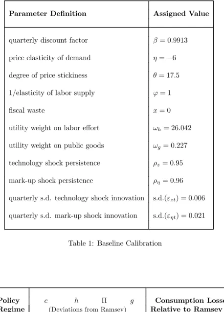
The baseline calibration of the model is summarized in table 1. The quarterly discount factorβ is chosen to match the average ex-post U.S. real interest rate during the period 1983:1-2002:4, i.e.,3.5%. The steady state value for the price elasticity of demand η is set at ₋6, implying a mark-up over marginal cost of 20%. The degree of price stickiness θ is chosen to be 17.5, such that the log-linearized version of the Phillips curve (8) is consistent with the estimates of Sbordone (2002), as in Schmitt-Grohé and Uribe (2004a). The elasticity of labor effort is assumed to be one (ϕ= 1) and we abstract from wasteful fiscal spending, i.e.,x= 0. The utility weightsωhandωg are chosen such that in the Ramsey steady state agents work 20% of their time(h= 0.2)and spend 20% of output on public goods(g= 0.04).9 _{The process for the technology shockz}

tis

8_{As before, we abstract from non-stationary components of time zero optimal policies in} the solution to (OI).

9_{The values ofω}

handωgare set according to equations (47) and (48), respectively, derived

taken from Schmitt-Grohé and Uribe (2004a).10 The parameterization for the mark-up shock processηtis taken from Ireland (2004).11

To test the robustness of our results, we consider also a range of alternative model parameterizations. For comparability, the utility weightsωh and ωg are adjusted so as to leave the Ramsey steady state unchanged.

The actual computational method we employ to numerically solve for the Markov-perfect Nash equilibrium with sequential monetary and fiscal policy is described in appendix A.7. A useful by-product of this approach is that it delivers second-order accurate welfare expressions for economies with a distorted steady state, while relying on linear-quadratic approximation only. This will be useful in section 8 when we analyze a stochastic economy.

6

Steady State Outcomes

Employing the baseline calibration summarized in table 1, we now investigate the quantitative impact of relaxing monetary andfiscal policy commitment. In addition, we compare the outcome under sequential policy (SP) to that achieved under the optimal inflation (OI) regime. Finally, we analyze the robustness of the quantitativefindings to different model parameterizations.

Thefirst row of table 2 presents information on the steady state in the SP regime. All variables are expressed as percentage deviations from their corre-sponding Ramsey steady state values.12 _{The last column of the table reports}

the steady state welfare loss, expressed in terms of the permanent reduction in private consumption that would imply the Ramsey steady state to be welfare equivalent to the considered policy regime, see appendix A.8 for details. In line with proposition 2, the sequential policy outcome is characterized by an inflation bias, which turns out to be sizable. In addition, there is a small fiscal spending bias. Overall, the welfare losses generated by the sequential conduct of policy are sizable, in the order of 1% of steady state consumption per period. The second row of table 2 shows the outcome under the OI regime. The optimal inflation rate turns out to be not only lower than the one in the SP regime but also very close to the Ramsey value. Note that reducing inflation from the level of the SP regime to the optimal level increases thefiscal spending bias, as suggested by proposition 4. While the fiscal spending increase asso-ciated with bringing down inflation is fairly large, implementing the optimal

1 0_{To transform the annual values reported in table 1 of Schmitt-Grohé and Uribe (2004a),} we raise the AR-coefficient of the technology shock to the power 1/4 and divide the standard deviation of the shock innovation by 4.

1 1_{Table 1 in Ireland (2004) presents estimates for the scaled mark-up shock process} ηt

θ.

Multiplying his estimate for the standard deviation by our price adjustment costθ= 17.5

yields the standard deviation in our table 1. Ireland’s estimate for the technology shock process is similar to the one used in this paper.

inflation rate nevertheless eliminates large part of the welfare losses associated with the SP regime. This suggests that thefiscal spending bias, despite being sizable in absolute value, is not very detrimental in welfare terms. Clearly, this result hinges partly on the assumed availability of lump sum taxes, which ab-stracts from deadweight losses typically associated with having tofinancefiscal expenditure.13

The results from table 2 suggest that installing a conservative monetary au-thority is desirable - despite the lack offiscal commitment - because the optimal inflation rate is well below the one emerging in the SP regime. Moreover, a conservative monetary authority can possibly eliminate large part of the welfare losses associated with sequential monetary andfiscal policymaking.

Table 3 explores the robustness of thesefindings to a wide range of changes in the parameterization of the model.14 The table reports the steady state welfare losses associated with the different policy regimes (first column) and the difference between inflation in the SP regime and the optimal inflation rate (second column). The previousfindings seem fairly robust. In particular, sig-nificant welfare gains can be realized from implementing the optimal inflation rate. Exceptions are theflexible price limit(θ_→0)and the cases with inelastic labor supply (large values forϕ), since the time-inconsistency problems of mon-etary andfiscal policy then disappear and real allocations approach the Ramsey steady state. The fact that all parameterizations display a positive inflation dif-ferential in the last column of table 3 suggests a conservative monetary authority should be desirable. We investigate this issue in detail in the next section.

7

Conservative Monetary Authority

This section analyzes whether the steady state distortions stemming from se-quential monetary andfiscal policy decisions can be reduced by installing a cen-tral bank that is more inflation averse than society. Rogoff(1985) and Svensson (1997) have shown this to be the case iffiscal policy is treated as exogenous.

Following Rogoff (1985), we consider a ‘weight conservative’ monetary au-thority with period utility function

(1₋α)u(ct+j, ht+j, gt+j)−α

(Πt−1)2 2

whereα_∈[0,1]is a measure of monetary conservatism. For α >0the mone-tary authority dislikes inflation (and deflation) more than society; if α= 1the

1 3_{A version of the model with distortionary labor taxes suggests that larger welfare losses} are associated with lack offiscal commitment.

1 4_{For all parametrization considered in table 3, the utility weightsω}

handωg are adjusted

to leave the Ramsey steady state unchanged. When considering wastefulfiscal expenditure

policymaker cares about inflation only. The preferences of the fiscal authority remain unchanged.

With monetary and fiscal authorities now pursuing different policy objec-tives, the equilibrium outcome will depend on the timing of policy moves, i.e., whetherfiscal policy is determined before, after, or simultaneously with mone-tary policy. It remains to be ascertained, however, which of these timing struc-tures is the most relevant for actual economies. While it may take long to implementfiscal policies, the time lag between a monetary policy decision and its effect on the economy can also be substantial. We thus consider Nash as well as leadership equilibria.

7.1

Nash and Leadership Equilibria

This section defines the various equilibria then briefly discusses them.

Consider the case of simultaneous policy decisions first. While the policy problem of thefiscal authority is unchanged, the monetary authority now solves

max {ct+j,ht+j,Πt+j,Rt+j≥1} Et ∞ X j=0 βj³(1₋α)u(ct+j, ht+j, gt+j)− α 2(Πt−1) 2´ (19) s.t.

Equations (8),(9),(10) for allt

{ct+j, ht+j,Πt+j, Rt+j≥1, gt+j−1} given forj≥1

As shown in appendix A.9, the first order conditions associated with problem (19) deliver the conservative monetary authority’s reaction function

−z_utuct ht (ηt(Πt−1)−Πt)−(Πt−1)ηt µ 1 +ht uhht uht ¶ + ∙ 2Πt−1− ucct uct (Πt−1) (θ(Πt−1)Πt−ztht(1 +ηt)) ¸_{(1−α)θ−α}zt uht (1₋α)θ+α_u1_ct = 0 (CMRF) Forα= 0, CMRF reduces to the monetary reaction function without conser-vatism (MRF).15 _{This motivates the following definition.}

Definition 5 (CSP-Nash) A Markov-perfect Nash equilibrium with sequen-tial and conservative monetary policy, sequensequen-tial fiscal policy and simultaneous policy decisions is a sequence _{ct, ht,Πt, Rt, gt} solving (8), (9), (10), (FRF)

and (CMRF).

1 5_{As before, CMRF implies that current interest rates depend on current economic} condi-tions only, validating the conjecture in (19) that in a Markov-perfect equilibrium future policy choices can be taken as given.

Next, we consider the case of monetary leadership (ML). The conservative monetary authority must take into account how thefiscal authority will react to its own decisions, i.e., FRF needs to be imposed as additional constraint. The monetary authority’s policy problem at timetis thus given by

max {ct+j,ht+j,Πt+j,Rt+j≥1,gt+j} Et ∞ X j=0 βj³(1₋α)u(ct+j, ht+j, gt+j)− α 2(Πt+j−1) 2´ (20) s.t.

Equations (8),(9),(10),(FRF) for allt

{ct+j, ht+j,Πt+j, Rt+j ≥1, gt+j} given forj≥1

The first order conditions associated with problem (20) deliver the conserva-tive monetary reaction function with monetary leadership, that we denote by CMRF-ML. This gives rise to the following definition.

Definition 6 (CSP-ML) A Markov-perfect equilibrium with sequential and conservative monetary policy, sequential fiscal policy and monetary policy de-ciding beforefiscal policy is a sequence_{ct, ht,Πt, Rt, gt}solving (8), (9), (10),

(FRF) and (CMRF-ML).

Finally, we consider the case of fiscal leadership (FL). The fiscal authority must now take into account the conservative monetary authority’s reaction, i.e., CMRF. Thefiscal authority’s policy problem at timetis thus given by

max {ct+j,ht+j,Πt+j,Rt+j≥1,gt+j} Et ∞ X j=0 βju(ct+j, ht+j, gt+j) (21) s.t.

Equations (8),(9),(10), (CMRF) for allt

{ct+j, ht+j,Πt+j, Rt+j ≥1, gt+j} given forj≥1

Thefirst order conditions associated with problem (21) deliver the corresponding fiscal reaction function that we denote by CFRF-FL. We propose the following definition.

Definition 7 (SCMFP-FL) A Markov-perfect equilibrium with sequential and conservative monetary policy, sequentialfiscal policy, and fiscal policy deciding before monetary policy is a sequence _{ct, ht,Πt, Rt, gt} solving (8), (9), (10),

(CFRF-FL) and (CMRF).

We now briefly comment on the previous definitions. First, note that for the caseα= 0all three equilibria reduce to the standard SP regime considered before in section 6. Second, for the Nash and monetary leadership cases, there

exists a theoretical upper bound on the welfare gains that monetary conser-vatism can possibly achieve. In these cases thefiscal authority takes monetary decisions as given, implying that FRF continues to describefiscal behavior. The best possible allocation is thus described by the solution to the OI regime of sec-tion 4.4. Third, in the case withfiscal leadership, thefiscal authority anticipates the monetary reaction function. Monetary policy may then use ‘off-equilibrium’ behavior to discipline the behavior of thefiscal authority along the equilibrium path. Fiscal leadership thus opens the possibility for outcomes that are welfare superior to those achieved in the OI regime.

7.2

Implications of Central Bank Conservatism

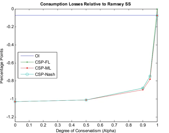
Figure 1 displays the steady state welfare gains associated with different degrees of monetary conservatism α _∈ [0,1], under the different leadership arrange-ments.16 _{The upper horizontal line shown in the figure indicates the welfare}

losses of the OI regime. Without monetary conservatism (α= 0) all leadership arrangements deliver the welfare loss associated with the SP regime.

For the Nash and monetary leadership (ML) regimes, a fully conservative monetary authority (α= 1) approximately implements the steady state welfare level associated with the OI regime.17 _{With an appropriate degree of monetary}

conservatism it is possible to recover the significant welfare losses resulting from lack of monetary commitment, in the order of 1% of steady state consumption per period. Interestingly, most of the welfare gains are achieved for values of α above 0.9, i.e., by a sufficiently conservative central bank caring almost exclusively about inflation.

The case for a conservative monetary authority is even stronger under the fiscal leadership (FL) regime. As shown in figure 1, a conservative monetary authority can recover not only the steady state welfare losses stemming from sequential monetary decision making, but also those emerging from lack offiscal commitment. With full conservatism (α = 1) the central bank recovers the Ramsey steady state. Again, most of the welfare gains are realized for values of

αabove 0.9.

Fiscal leadership differs from the Nash and monetary leadership cases be-cause thefiscal authority anticipates the reaction of the conservative monetary authority. Forα= 1, the monetary authority is determined to implement price stability at all costs. Afiscal expansion above the Ramsey spending level would generate inflationary pressures, triggering a strong increase in interest rates so as to reduce private consumption. The fiscal authority anticipates that fiscal spending simply results in a crowding out of private consumption, this disci-plines its behavior.

1 6_{This and subsequentfigures use the baseline calibration of section 5.}

1 7_{As will become clear from figure 2 below, the welfare level of the OI regime is actually} achieved by a value ofαvery close but slightly below 1.

Figure 2 illustrates for the different leadership cases how the steady state val-ues of private consumption, labor effort, inflation and public spending depend on the degree of monetary conservatism. While increased monetary conser-vatism reduces the inflation bias for all timing protocols, its effect on thefiscal spending bias depends on whether or notfiscal policy anticipates the monetary policy reaction. If fiscal policy takes monetary decisions as given, monetary conservatism results in an increasedfiscal spending bias. Withfiscal leadership, however,fiscal spending decreases to the Ramsey level asαincreases towards 1. A value ofα= 1recovers the Ramsey outcome in the FL regime, while a value ofαslightly below one recovers the OI outcome in the Nash and ML regimes.

8

Conservatism and the Response to Shocks

Up to this point we have restricted attention to steady state outcomes. This section extends the analysis to a stochastic economy, considering how stabiliza-tion policy is affected by different monetary andfiscal policy regimes and the degree of monetary conservatism.

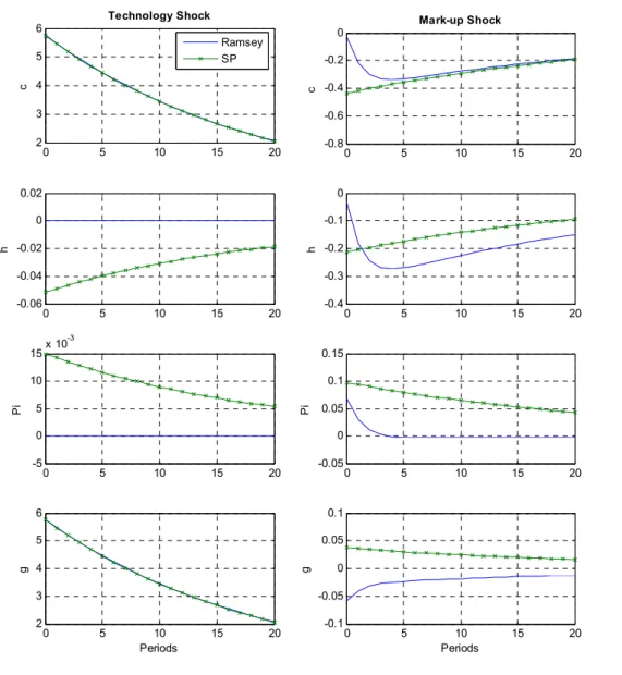
Figure 3 depicts impulse responses to a positive technology shock (left col-umn) and positive mark-up shock (right colcol-umn) for the case with commitment and under sequential policy.18 Thefigure illustrates that lack of monetary and fiscal commitment influences the impulse responses markedly. Under commit-ment inflation either reacts not at all (technology shocks) or just by a small amount (mark-up shocks). Instead, inflation increases by more and is also more persistent under sequential policy. Intuitively, positive technology shocks in-crease the temptation to boost the suboptimally low level of labor supply by ‘surprise inflation’, because labor input is temporarily more productive. Sim-ilarly, positive mark-up shocks temporarily increase the labor supply wedge, thereby also strengthen the incentives to raise labor input through additional fiscal spending.

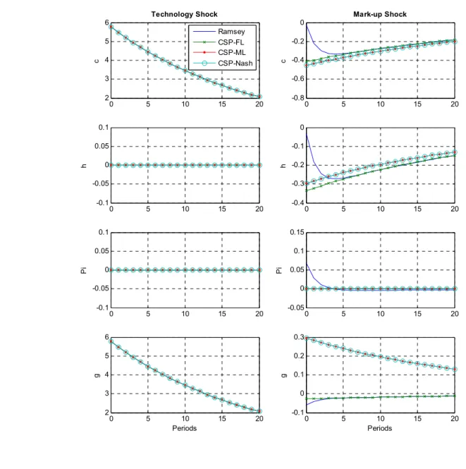
Figure 4 clarifies how impulse responses are affected by installing an infl a-tion conservative central bank. Thefigure depicts the Ramsey policy response together with the responses for the Nash and two leadership cases (ML and FL), assuming a fully conservative central bank focusing on inflation only (α= 1). The left column of thefigure shows that full monetary conservatism causes the sequential policy response to productivity shocks to be identical to the response under commitment, for all timing protocols. Full monetary conservatism imple-ments the optimal stabilization policy in response to technology shocks, despite the sequential conduct of monetary andfiscal policy.

Next, consider the case of mark-up shocks, depicted in the right column of figure 4. Under fiscal leadership (FL) impulse responses deviate somewhat

1 8_{Using the baseline calibration of section 5 we consider a positive 3 standard deviation} disturbance for the technology and mark-up shock values. Responses are presented in terms of percent deviations from steady state values.

from the Ramsey policy response, but deviations tend to be short-lived and smaller than in the case without conservatism, compare with figure 3. With monetary leadership (ML) or simultaneous policymaking (Nash) the situation is largely similar, except for the response of government spending, which then differs markedly from the Ramsey policy response. The discussion in section 6 suggests, however, that deviations of government spending from its optimal level do not have significant effects on welfare in the current setting.19

The previousfindings suggest that monetary conservatism remains desirable in a stochastic economy because welfare effects tend to be dominated by steady state considerations. Moreover, monetary conservatism quite surprisingly -also tends to improve the conduct of stabilization policy, especially in response to technology shocks. Clearly, further welfare gains could be achieved through even better stabilization policies.

9

Conclusions

This paper analyzes monetary andfiscal policy interactions in a dynamic sto-chastic general equilibrium model when policymakers lack the ability to credibly commit to policies ex-ante. It is shown that lack offiscal commitment leads to excessivefiscal spending on public goods, while lack of monetary commitment results in the well-known inflation bias. The welfare losses generated by the sequential conduct of monetary andfiscal policy appear to be substantial.

While optimal monetary policy that appropriately internalizes the fiscal spending distortion implements positive inflation, we find the optimal infl a-tion rate for our baseline calibraa-tion to be close to zero. Also, for a wide range of model parameterizations, the monetary inflation bias results larger than the optimal inflation rate, causing monetary conservatism to remain desirable in a situation with endogenousfiscal spending.

Wefind that large part of the steady state welfare losses associated with lack of monetary andfiscal commitment can be recouped, provided the monetary au-thority focuses exclusively on stabilizing inflation. Moreover, a fully conservative monetary authority also tends to improve the conduct of stabilization policy.

A number of important questions remain to be addressed in further research. In particular, for a positive description of monetary andfiscal policy interactions, it seems important to consider also distortionary taxation and government debt dynamics. These elements introduce additional interactions between monetary andfiscal policymakers that may have a major impact on the desirability of an inflation conservative monetary authority. We plan to extend the analysis to such richer settings in future work.

1 9_{Indeed, computing how consumption equivalent welfare losses depend on the degree of} monetary conservatismαin a stochastic economy, results are virtually unchanged when com-pared tofigure 1, which is based on a steady state comparison.

A

Appendix

A.1

Ramsey Steady State

The Lagrangian of the Ramsey problem (12) is max {ct,ht,Πt,Rt,gt} E0 ∞ X t=0 βtnu(ct, ht, gt) +γ_t1 ∙ uct(Πt−1)Πt− uctztht θ µ 1 +ηt+ uht uct ηt zt ¶ −βuct+1(Πt+1−1)Πt+1 ¸ +γ_t2 ∙ uct Rt − βuct+1 Πt+1 ¸ +γ_t3 ∙ ztht−ct− θ 2(Πt−1) 2 −gt−x ¸¾

Thefirst-order conditions w.r.t. (ct, ht,Πt, Rt, gt), respectively, are given by

uct+γt1 µ ucct(Πt−1)Πt− ucctztht θ (1 +ηt) ¶ −γ_t1₋₁ucct(Πt−1)Πt+γt2 ucct Rt − γ_t2₋₁ucct Πt − γ3_t = 0 (22) uht−γt1 uctzt θ µ 1 +ηt+ uht uct ηt zt +ht uhht uct ηt zt ¶ +γ3 tzt= 0 (23) ¡ γ_t1₋γ1_t−1¢uct(2Πt−1) +γt2−1 uct Π2 t − γ_t3θ(Πt−1) = 0 (24) −γ_t2uct R2 t = 0 (25) ugt−γ3t = 0 (26) where γ₋j₁ = 0for j = 1,2. We denote the Ramsey steady state by dropping time subscripts. Equation (25),uct>0andRt≥1imply

γ2= 0 Equations (26) delivers

γ3=ug>0 This and equation (24) gives

Π= 1 From (9) it then follows

R= 1

β

Then equation (8) delivers

1 +η+uh

uc

This delivers (13) shown in the main text. Using the previous results, equation (23) simplifies to

uh−γ1

h

θuhhη+ug= 0 (28)

From (22) one obtains

γ1h θ =

uc−ug

ucc(1 +η)

(29) Substituting (29) into (28) delivers

uh−

uc−ug

ucc(1 +η)

uhhη+ug= 0 Using (27) to substitute foruc one gets

ug=−uh 1 +³₁₊η_η´ 2 uhh ucc 1 +₁₊η_ηuhh ucc

Using (27) again to substitute ₁₊η_η delivers (14) shown in the main text.

A.2

Sequential Fiscal Reaction Function

Thefiscal problem (15) is

max {ct+j,ht+j,Πt+j,gt+j} Et ∞ X j=0 βjnu(ct+j, ht+j, gt+j) +γ_t1_+j ∙ uct+j(Πt+j−1)Πt+j− uct+jzt+jht+j θ µ 1 +ηt+j+ uht+j uct+j ηt+j zt+j ¶ − βuct+j+1(Πt+j+1−1)Πt+j+1 i +γ_t2_+j ∙ uct+j Rt+j − βuct+j+1 Πt+j+1 ¸ +γ3_t+j ∙ zt+jht+j−ct+j− θ 2(Πt+j−1) 2 −gt+j−x ¸¾

taking as givenRt+j−1and other variables datedt+j forj≥1. Thefirst order

conditions w.r.t. (ct, ht,Πt, gt), respectively, are given by

uct+γ1t µ ucct(Πt−1)Πt− ucctztht θ (1 +ηt) ¶ +γ_t2ucct Rt − γ_t3= 0 (30) uht−γ1t uctzt θ µ 1 +ηt+ uht uct ηt zt +ht uhht uct ηt zt ¶ +γ_t3zt= 0 (31) γ_t1uct(2Πt−1)−γt3θ(Πt−1) = 0 (32) ugt−γt3= 0 (33)

From equations (32) and (33) one gets

γ_t1=ugtθ(Πt−1)

uct(2Πt−1)

Using the previous result and (33) to substitute the Lagrange multipliers in (31) delivers FRF shown in the main text.

A.3

Sequential Monetary Reaction Function

The monetary problem (17) is max {ct+j,ht+j,Πt+j,Rt+j} Et ∞ X j=0 βjnu(ct+j, ht+j, gt+j) +γ_t1_+j ∙ uct+j(Πt+j−1)Πt+j− uct+jzt+jht+j θ µ 1 +ηt+j+ uht+j uct+j ηt+j zt+j ¶ − βuct+j+1(Πt+j+1−1)Πt+j+1 i +γ_t2_+j ∙ uct+j Rt+j − βuct+j+1 Πt+j+1 ¸ +γ3t+j ∙ zt+jht+j−ct+j− θ 2(Πt+j−1) 2 −gt+j−x ¸¾

taking as givengt+j−1and other variables datedt+j forj≥1. Thefirst order

conditions w.r.t. (ct, ht,Πt, Rt)are given by

uct+γ1t µ ucct(Πt−1)Πt− ucctztht θ (1 +ηt) ¶ +γ_t2ucct Rt − γ_t3= 0 (34) uht−γ1t uctzt θ µ 1 +ηt+ uht uct ηt zt +ht uhht uct ηt zt ¶ +γ_t3zt= 0 (35) γt1uct(2Πt−1)−γt3θ(Πt−1) = 0 (36) −γ_t2uct R2 t = 0 (37)

Equation (37),uct>0andRt≥1imply

γ_t2= 0

Then solving (34), (35) and (36) forγ_t3 delivers, respectively,

γ_t3=uct+γt1 µ ucct(Πt−1)Πt− ucctztht θ (1 +ηt) ¶ (38) γ_t3=₋uht zt +γ1_tuct θ µ 1 +ηt+ uht uct ηt zt +ht uhht uct ηt zt ¶ (39) γt3=γt1 uct(2Πt−1) θ(Πt−1) (40)

Equations (38) and (40) imply γt1= θ 2Πt−1 Πt−1 − ucct uct (θ(Πt−1)Πt−ztht(1 +ηt)) (41) While equations (39) and (40) give

γ1_t = θ ztuct uht ³ 1 +ηt−2Π_Πtt₋−₁1+_uu_cthtη_zt_t +htu_uhht_ct η_ztt ´ (42)

From (41) and (42) one obtains MRF shown in the main text.

A.4

Proof of Proposition 2

Wefirst show that MRF cannot hold in the neighborhood of Π= 1. In steady state one can rewrite MRF as

Π µ 1 + uc uh ¶ +O(Π₋1) = 0 (43)

where O(Π₋1) summarizes terms that converge to zero as (Π₋1) _→ 0. In a steady state with Π = 1 equation (8) delivers 1 +η+ uh

ucη = 0 and thus

uc

uh < −

η

1+η < −1. Since the implicit function uc

uh(Π) defined by (8) exists,

this implies that 1 + uc

uh is bounded away from −1 also in a sufficiently small

neighborhood aroundΠ= 1. Therefore, (43) cannot hold in the neighborhood ofΠ= 1. Moreover, fromR_≥1and (9) we haveΠ_≥β in steady state. Forβ

sufficiently close to 1, it then follows that MRF can only hold ifΠ>1.

A.5

Proof of Proposition 4

The effect of inflation on steady state utility is given by

du dΠ =uc ∂c ∂Π+uh ∂h ∂Π+ug ∂g ∂Π (44)

where c(Π), h(Π), g(Π) denote the steady state levels emerging under sequen-tial fiscal policy when monetary policy implements inflation rate Π, and the derivativesuj (j =c, h, g)are evaluated at this steady state. Wefirst evaluate equation (44) atΠ= 1. Equation (8) simplifies to

uc=−

η

1 +ηuh (45)

Totally differentiating equation (10) and evaluating atΠ= 1 gives

∂c ∂Π = ∂h ∂Π− ∂g ∂Π

Using this result and (16), equation (44) can be rewritten as

du

dΠ = (uc−ug)

∂c ∂Π

Equations (16) and (45) implyuc> ug, thus sign µ du dΠ ¶ =sign µ ∂c ∂Π ¶ (46) To determine the sign of ∂c/∂Π we totally differentiate equations (FRF), (8), (10) and evaluate atΠ= 1, this delivers

⎛ ⎝ 0 ₋uhh −ugg h θη uhucc u2 c − h θη uhh uc 0 −1 1 ₋1 ⎞ ⎠ ⎛ ⎝ ∂c ∂Π ∂h ∂Π ∂g ∂Π ⎞ ⎠= ⎛ ⎝ hη uhuhh uc 0 0 ⎞ ⎠

Solving for _∂∂c_Π and _∂∂g_Π gives

∂c ∂Π = ucuhh ucuhhugg−uccuhugg−uccuhuhh hηuhuhh uc ∂g ∂Π = −ucuhh+uccuh ucuhhugg−uccuhugg−uccuhuhh hηuhuhh uc

Assuminguhh <0, signing these expression delivers _∂∂c_Π > 0 and _∂∂g_Π < 0, as claimed. The former inequality and equation (46) imply du

dΠ > 0, locally at

Π= 1.

A.6

Utility Weights

For the period utility specification (18), the Ramsey policy marginal conditions (13) and (14), respectively, deliver

ωh= 1 chϕ 1 +η η (47) ωg=ωhghϕ 1 + ₁₊η_ηhcϕ 1 + c hϕ (48) Assuming c = 0.16, h = 0.2, g = 0.04, η = ₋6 and ϕ = 1 one obtains the parameter values in table 1.

A.7

Solving for the Equilibrium with Sequential

Mone-tary and Fiscal Policy

The Markov-perfect Nash equilibrium with sequential monetary andfiscal policy solves the following problem

max {ct+j,ht+j,Πt+j,Rt+j,gt+j} Et ∞ X j=0 βju(ct+j, ht+j, gt+j) (49) s.t.

Equations (8),(9),(10) for allt

One should note that FRF and MRF need not be imposed, since they can already be derived from thefirst order conditions of this problem, see sections 4.3.1 and 4.3.2, respectively. Therefore, the solution of problem (49) will always satisfy FRF and MRF.

Then, the recursive formulation of the Lagrangian of problem (49) is

W(zt, ηt) = min (γ1 t,γ2t,γt3) max (ct,ht,Πt,Rt,gt){ f(_·) +βEtW(zt+1, ηt+1)} (50) s.t. zt+1= (1−ρz) +ρzzt+εzt+1 ηt+1=η(1−ρη) +ρηηt+εηt+1

where the one-period return is

f(_·) =u(ct, ht, gt) +γ_t1 ∙ uct(Πt−1)Πt− uctztht θ µ 1 +ηt+ uht uct ηt zt ¶ −EAS_t ¸ +γ_t2 ∙ uct Rt − E_tIS ¸ +γ_t3 ∙ ztht−ct− θ 2(Πt−1) 2 −gt−x ¸

with the expectations functions

EtAS ≡βEtuct+1(Πt+1−1)Πt+1 (51) EIS t ≡βEt uct+1 Πt+1 (52) taken as given. The additional control variablesγ1

t, γt2, γt3 are the Lagrange multipliers associated with the implementability constraints (8) and (9), and the feasibility constraint (10), respectively.

We then solve for the steady state using the first order conditions of the recursive formulation (50). Thereafter, we compute a quadratic approximation of the one-period returnf(_·) around this steady state. This involves quadrat-ically approximating the implementability and feasibility constraints. Instead, the expectation functionsEAS

t andEtIS are linearly approximated as

E_tAS _≈a1₀+a1₁(zt−1) +a12(ηt−η) (53)

E_tIS _≈a2₀+a2₁(zt−1) +a22(ηt−η) (54) Importantly, postulating linear expectation functions is sufficient to obtain a first order approximation to the equilibrium dynamics and policy functions. The policymaker takes expectations functions as given, therefore, they do not show up in differentiated form in the first order conditions. Moreover, linear

expectations functions are sufficient to evaluate the Lagrangian, i.e., utility, up to second order. This is the case since either the implementability constraints or the associated Lagrange multipliers are zero in a sufficiently small neighborhood around the steady state. As a result, nofirst order terms appear when evaluating the quadratic approximation off(_·) at the solution. Obviously, this is just a restatement of the fact that (50) is an unconstrained optimization problem.

We now explain how we compute the expectation functions (53) and (54). We start with an initial guess for aj_i (j = 1,2; i = 0,1,2), then we solve (50) withf(_·)replaced by its quadratic approximation. We updateαj_i, as explained below, and continue iterating until the maximum absolute change of the policy functions drops below the square root of machine precision, i.e.,1.49_·10−8_.

Let the solution for the policy functionsc(_·)andΠ(_·)be given by

ct+1−c=δcz(zt+1−1) +δcη(ηt+1−η) (55)

Πt+1−Π=δΠz(zt+1−1) +δΠη(ηt+1−η) (56)

where variables without time subscript denote steady state values. Afirst order approximation of the expectation functions (51) and (52) then delivers

EtAS ≈ EASt ¯ ¯ ss+ ∂EAS t ∂ct+1 ¯ ¯ ¯ ¯ ss Et(ct+1−c) + ∂EAS t ∂Πt+1 ¯ ¯ ¯ ¯ ss Et(Πt+1−Π) E_tIS _≈ EIS_t ¯¯_ss+ ∂E IS t ∂ct+1 ¯ ¯ ¯ ¯ ss Et(ct+1−c) + ∂EIS t ∂Πt+1 ¯ ¯ ¯ ¯ ss Et(Πt+1−Π)

where_|ss indicates expressions evaluated at steady state. These together with (55), (56) and

Et(zt+1−1) =ρz(zt−1)

Et(ηt+1−η) =ρη(ηt−η)

deliver the expectations functions consistent with the approximated policy func-tions a1 0=βuc(Π−1)Π a1 1=βρz[(Π−1)Πuccδcz+uc(2Π−1)δΠz] a1 2=βρη[(Π−1)Πuccδcη+uc(2Π−1)δΠη] a2 0=βuΠc a2 1=β ρz Π £ uccδcz−u_ΠcδΠz¤ a2 2=β ρη Π £ uccδcη−u_ΠcδΠη¤

A.8

Consumption Losses Relative to Ramsey

Let u(c, h, g) denote the period utility for the Ramsey steady state and let

policy regime. The permanent reduction in private consumption that would imply the Ramsey steady state to be welfare equivalent to the alternative policy regimeµA_{≤0is implicitly defined by}

1 1₋βu ¡ cA, hA, gA¢= 1 1₋βu ¡ c(1 +µA), h, g¢ = 1 1₋β £ u(c, h, g) + log¡1 +µA¢¤

where the second equality uses equation (18). Therefore, one obtains

µA= exp£u¡cA, hA, gA¢₋u(c, h, g)¤₋1

A.9

Conservative Monetary Reaction Function

The conservative monetary problem (19) is max {ct+j,ht+j,Πt+j,Rt+j} Et ∞ X j=0 βjn(1₋α)u(ct+j, ht+j, gt+j)− α 2(Πt−1) 2 +γ_t1_+j ∙ uct+j(Πt+j−1)Πt+j− uct+jzt+jht+j θ µ 1 +ηt+j+ uht+j uct+j ηt+j zt+j ¶ − βuct+j+1(Πt+j+1−1)Πt+j+1 i +γ_t2_+j ∙ uct+j Rt+j − βuct+j+1 Πt+j+1 ¸ +γ3_t+j ∙ zt+jht+j−ct+j− θ 2(Πt+j−1) 2 −gt+j−x ¸¾

taking as given gt+j−1 and variables dated t+j for j ≥ 1. The first order

conditions w.r.t. (ct, ht,Πt, Rt), respectively, are given by (1₋α)uct+γt1 µ ucct(Πt−1)Πt− ucctztht θ (1 +ηt) ¶ +γ_t2ucct Rt − γ_t3= 0 (57) (1₋α)uht−γt1 uctzt θ µ 1 +ηt+ uht uct ηt zt +ht uhht uct ηt zt ¶ +γ3tzt= 0 (58) γt1uct(2Πt−1)−γt3θ(Πt−1)−α(Πt−1) = 0 (59) −γ2 t uct R2 t = 0 (60) Equation (60),uct>0andRt≥1imply

Then solving (57), (58) and (59) forγt3 delivers, respectively, γ_t3= (1₋α)uct+γt1 µ ucct(Πt−1)Πt− ucctztht θ (1 +ηt) ¶ (61) γ_t3=₋(1₋α)uht zt +γ_t1uct θ µ 1 +ηt+ uht uct ηt zt +ht uhht uct ηt zt ¶ (62) γ_t3=γ1_tuct(2Πt−1) θ(Πt−1) − α θ (63)

Equations (61) and (63) imply

γt1= θ³1₋α+_u1 ct α θ ´ 2Πt−1 Πt−1 − ucct uct (θ(Πt−1)Πt−ztht(1 +ηt)) (64) While equations (62) and (63) give

γ1t = θ³1₋α₋ zt uht α θ ´ ztuct uht ³ 1 +ηt−2ΠΠtt−−11+ uht uct ηt zt +ht uhht uct ηt zt ´ (65)

References

Alesina, Alberto and Guido Tabellini, “Rules and Discretion with Non-coordinated Monetary and Fiscal Policies,” Economic Inquiry, 1987, 25, 619—630.

Barro, Robert and David B. Gordon, “A Positive Theory of Monetary Policy in a Natural Rate Model,” Journal of Political Economy, 1983,91, 589—610.

Chari, V. V. and Patrick J. Kehoe, “Sustainable Plans,”Journal of Polit-ical Economy, 1990,98, 783—802.

and , “Optimal Fiscal and Monetary Policy,” in John Taylor and Michael Woodford, eds., Handbook of Macroeconomics, Amsterdam: North-Holland, 1999, chapter 26.

Díaz-Giménez, Javier, Giorgia Giovannetti, Ramon Marimon, and Pedro Teles, “Nominal Debt as a Burden on Monetary Policy,”Pompeu Fabra University Mimeo, 2006.

Ferrero, Andrea, “Fiscal and Monetary Rules for a Currency Union,” ECB Working Paper No. 502, 2005.

Galí, Jordi and Tommaso Monacelli, “Optimal Monetary and Fiscal Policy in a Currency Union,”NBER Working Paper No. 11815, 2005.

Ireland, Peter, “Technology Shocks in the New Keynesian Model,”Review of Economics and Statistics, 2004, 86(4), 923—936.

Klein, Paul, Per Krusell, and José-Víctor Ríos-Rull, “Time Consistent Public Expenditures,”CEPR Discussion Paper No. 4582, 2004.

Kydland, Finn E. and Edward C. Prescott, “Rules Rather Than Discre-tion: The Inconsistency of Optimal Plans,”Journal of Political Economy, 1977,85, 473—492.

Leeper, Eric M., “Equilibria under Active and Passive Monetary and Fiscal Policies,”Journal of Monetary Economics, 1991,27, 129—147.

Lucas, Robert E. and Nancy L. Stokey, “Optimal Fiscal and Monetary Policy in an Economy Without Capital,”Journal of Monetary Economics, 1983,12, 55—93.

Ramsey, Frank P.,