Wall-Modeled Large Eddy Simulation of a Three-Dimensional Shock-Boundary Layer Interaction

(1)

Air Force Institute of Technology

AFIT Scholar

Theses and Dissertations Student Graduate Works

3-23-2018

Wall-Modeled Large Eddy Simulation of a

Three-Dimensional Shock-Boundary Layer Interaction

Nicholas J. Marco

Follow this and additional works at:https://scholar.afit.edu/etd

Part of theAerodynamics and Fluid Mechanics Commons, and theFluid Dynamics Commons

This Thesis is brought to you for free and open access by the Student Graduate Works at AFIT Scholar. It has been accepted for inclusion in Theses and Dissertations by an authorized administrator of AFIT Scholar. For more information, please [email protected].

Recommended Citation

Marco, Nicholas J., "Wall-Modeled Large Eddy Simulation of a Three-Dimensional Shock-Boundary Layer Interaction" (2018).Theses and Dissertations. 1777.

(2)

Wall-Modeled Large Eddy Simulation of a Three-Dimensional Shock-Boundary Layer

Interaction

THESIS

Nicholas J. Marco, 2d Lt, USAF AFIT-ENY-MS-18-M-277

DEPARTMENT OF THE AIR FORCE AIR UNIVERSITY

AIR FORCE INSTITUTE OF TECHNOLOGY

Wright-Patterson Air Force Base, Ohio

DISTRIBUTION STATEMENT A

(3)

The views expressed in this document are those of the author and do not reflect the official policy or position of the United States Air Force, the United States Department of Defense or the United States Government. This material is declared a work of the U.S. Government and is not subject to copyright protection in the United States.

(4)

AFIT-ENY-MS-18-M-277

WALL-MODELED LARGE EDDY SIMULATION OF A THREE-DIMENSIONAL SHOCK-BOUNDARY LAYER INTERACTION

-THESIS

Presented to the Faculty

Department of Aeronautics and Astronautics Graduate School of Engineering and Management

Air Force Institute of Technology Air University

Air Education and Training Command in Partial Fulfillment of the Requirements for the Degree of Master of Science in Aeronautical Engineering

Nicholas J. Marco, B.S.M.E., E.I.T 2d Lt, USAF

March 19, 2018

DISTRIBUTION STATEMENT A

(5)

-THESIS

Nicholas J. Marco, B.S.M.E., E.I.T 2d Lt, USAF Committee Membership: Maj. J. R. Komives, PhD Chair Maj. D. S. Crowe, PhD Member Dr. M. F. Reeder, PhD Member

(6)

Abstract

The computational cost of direct simulation of turbulent flows is prohibitive at high Reynolds numbers; thus, methods such as RANS and LES are used in order to model relevant engineering flows computationally. However, these methods require a large number of cells near a solid boundary increasing the computational time. To circumvent this issue, models that eliminate this need for large cell counts near solid boundaries can be used. One such method utilizes a Wall-Modeled Large Eddy Sim-ulation (WM-LES). Of interest is how these wall models perform in comparison to a Wall-Resolved Large Eddy Simulation (WR-LES) and experimental results of a shock turbulent boundary layer interactions (STBLI) and specifically, whether equilibrium wall models are sufficient to resolve the oscillatory and hence non-equilibrium nature of these flows or whether a non-equilibrium model is necessary. To study this a swept compression ramp which produces a 3-D STBLI was simulated using a Wall-Modeled Large Eddy Simulation. It was found that an equilibrium model is insufficient in de-termining both large scale features such as separation and reattachment locations as well as specific flow quantities such as wall shear While a non-equilibrium model did better in predicting both large scale features and specific flow quantities. However, the non-equilibrium model produced a non-physical secondary reattachment leading to a need for further research into the specific model.

(7)

To my wife and family who have provided unwavering support throughout my time at AFIT.

(8)

Acknowledgements

Without the help of many people and organizations this research would not have been possible. I would like to express my sincere thanks to those that helped me at AFIT. Including, my advisor, Jeff Komives, for providing me with guidance, advice, and support throughout this project as well as my lab mates, Charles Shuff and Evan Oren, who provided help and friendly conversation. I would also like to thank those outside of AFIT that made this project possible: The University of Minnesota for the use and support of US3D, The Ohio State University for the wall-resolved data, the Department of Defense High Performance Computing Modernization Program (DoD HPCMP) for use of Topaz which made these simulations possible, and the Air Force Research Lab (AFRL) for support and funding.

(9)

List of Figures

Figure Page

1 Turbulent boundary layer with contours of density.

Direct numerical simulation of Pirozzoli and Bernadini[1] . . . 2

2 A 30 degree sweep, 22.5 degree compression swept-ramp as presented by Adler et al.[2]. . . 4

3 Energy spectrum for a turbulent flow.[3] . . . 8

4 Typical velocity profile for a turbulent boundary layer. . . 9

5 Hierarchy of Turbulence Models[4]. . . 12

6 Embedded wall-model grid showing probe location at 4 cells off the wall[5]. . . 20

7 Diagram of the collapse of separation, ramp corner, triple point, and reattachment to the VCO by Adler et al.[2] . . . 22

8 Diagram of cross-section of domain, in the x-y plane, showing the fillet at the downstream outflow. . . 26

9 Diagram of domain showing the baffle surface 4δ above the wall, as depicted in blue. . . 27

10 Cross-section of surface grid used in the WM-LES studies. . . 29

11 Cross-section of surface grid used in the DDES studies. . . 30

12 Boundary Conditions with x-y cross-section on the left and top down, x-z cross section on the right. . . 31

13 Depiction of locations where the mean surface quantities are extracted from. Contour colors are of skin friction coefficient for a WM-LES simulation. . . 37

14 Wall-normal grid convergence study mean surface quantities: z = 8δ. . . 38

15 Spanwise and streamwise grid convergence study mean surface quantities: z = 8δ . . . 39

(12)

Figure Page 16 One-dimensional wall-model grid convergence study

mean surface quantities: z = 8δ. . . 41 17 Log Layer matching of the LES grid with wall-model

probe identified. The von Karman constant, κ, is 0.41

and the integration constant, C, is 5.1. . . 43 18 Reynolds Stresses compared to incompressible profile of

DeGraaff and Eaton[6]. . . 44 19 Wall heating ofδ/40 WM-LES case . . . 45 20 Comparison of surface streamlines between WM-LES

and WR-LES (z is up)[2]. . . 46 21 Diagram depicting the collapse of the VCO for the

equilibrium WM-LES (z is up). . . 47 22 Comparison of surface streamlines between WM-LES

and experiment (z is down)[7]. . . 47 23 Comparison of mean surface statistics between

WM-LES and WR-LES of Adler et al.: z = 2δ. . . 50 24 Comparison of mean surface statistics between

WM-LES and WR-LES of Adler et al.: z = 4δ. . . 53 25 Comparison of mean surface statistics between

WM-LES and WR-LES of Adler et al.: z = 8δ. . . 54 26 Mean flow contours where lines are WM-LES and color

contours are WR-LES of Adler et al.: z = 8δ[2]. . . 56 27 Mean flow contours where dashed lines are WM-LES

and color contours are experimental PIV of Vanstone et

al.[7]. . . 57 28 Spectral Data with PSD as a function of Strouhal

number: Stδ =f δ/U∞. . . 59

29 Diagram depicting the collapse of the VCO for the

non-equilibrium WM-LES. . . 61 30 Comparison of mean surface statistics between

(13)

Figure Page 31 Root mean square of pressure fluctuations for the

wall-resolved study of Adler et al.[2]. . . 65 32 Diagram depicting the collapse of the VCO for DDES. . . 66 33 Comparison of mean surface statistics between DDES,

WM-LES and Wr-LES . . . 67 34 Comparison of spectral data between DDES and

WM-LES with PSD as a function of Strouhal number:

(14)

List of Tables

Table Page

1 Experimental, WR-LES, and WM-LES flow properties. . . 25 2 Grid spacing of WR-LES . . . 28 3 Grid Properties for wall-normal grid convergence study. . . 29

(15)

List of Symbols

Symbol Page Re Reynolds Number . . . 2 y Y-displacement . . . 2 + Wall-units . . . 2 Energy . . . 7 ν Kinematic viscosity . . . 7 κ Wavenumber . . . 7 uτ Friction velocity . . . 9

τw Wall shear stress . . . 9

ρ Density . . . 9

u Streamwise velocity . . . 10

κ von Karman Constant . . . 10

C Integration Constant . . . 10

vD van Driest Transformed . . . 11

w Value at wall . . . 11

U Vector of conserved variables . . . 15

Fj Flux Vector . . . 15

xj Direction indexing . . . 15

u Velocity in j-direction . . . 15

E Total specific energy . . . 15

p Static pressure . . . 15

δij Kronecker delta . . . 15

(16)

Symbol Page

q Heat conduction . . . 15

R Gas constant . . . 16

T Temperature . . . 16

γ Ratio of specific heats . . . 16

Sij Rate of strain tensor . . . 16

λ Bulk viscosity . . . 16

ˆ µ Effecitve viscosity . . . 16

ˆ κ Effecitve thermal conductivity . . . 16

µ Molecular component of viscosity . . . 17

µt Turbulent component of viscosity . . . 17

κ Molecular component of thermal conductivty . . . 17

κt Turbulent component of thermal conductivity . . . 17

U Filetered variable . . . 17

U0 Sub-filtered variable . . . 17

G Filter function . . . 17

∆ Filter width . . . 17

Q Wall-modeled vector of conserved variables . . . 19

G Wall-modeled flux vector . . . 19

(17)

-I. Introduction

1.1 Study of Turbulent Flows

The turbulent nature of many flows of engineering interest is important due to the flows increased ability to transfer momentum. This increased transfer of momentum at a solid boundary, such as the surface of an aircraft, leads to higher values of quantities such as drag, heat transfer, and mass transfer. These quantities play major roles in the performance of aircraft and thus it is important for engineers to accurately predict such values[8]. Turbulence has a continuous range of energetic scales in both time and length, in which the largest scales are heavily influenced by the geometry of the flow whereas the smallest scales are determined by the rate at which they receive energy from the larger scales[8]. The continuous range of turbulent length scales, decreasing in size to a solid boundary, can be seen in Figure 1.

When studying turbulent flows, the use of experimental facilities is often limiting due to short run-times, restricting methods of data collection, and the inability to replicate the exact flight conditions of interest[5]. Alternatively, one can use Computa-tional Fluid Dynamics (CFD) which solves the governing equations of fluid dynamics, the Navier-Stokes Equations, through discretization of the domain of interest. CFD can provide flexibility in the aforementioned areas which plague experiments such as reproducing exact flight conditions as well as the ability to obtain data from nearly

(18)

Figure 1. Turbulent boundary layer with contours of density. Direct numerical simu-lation of Pirozzoli and Bernadini[1]

any point in the flow. However, CFD present its own challenges, mainly: high com-putational cost for flows of engineering interest and the accuracy of models included in the numerics.

1.2 Simulation of Turbulent Flows

In order to simulate a turbulent flow with effectively no modeling, one would be required to use a Direct Numerical Simulation (DNS), which resolves all the scales of turbulence. However, DNS is extremely costly since the number of grid points needed to sufficiently resolve the smallest turbulent eddies scales as a function of the Reynolds number, Re9/4_{[9]. To circumvent this issue, turbulence models are used to model}

the smaller scales and therefore create a less costly computation. However, these models still require similar grid resolution requirements near solid boundaries, with a maximum height of the wall-adjacent cell limited to under one wall unit (y+ _≤ _1).

Where, y+ is a dimensionless wall distance of a wall-bounded flow. This limit is true of a Wall-Resolved Large Eddy Simulation (WR-LES). This clustering of small cells along the wall boundaries, or “near-wall problem,” decreases the size of the timestep that can be used therefore limiting the Reynolds number that can be studied. This restriction poses a problem to studying flows of engineering interest at high Reynolds numbers, such as hypersonic flows or full vehicle simulations.

(19)

Traditionally, Reynolds-Averaged Navier-Stokes (RANS) methods, in which the mean flow is solved, are used in such high Reynolds number cases. However, these methods have been found to be erroneous in more complex flows, such as turbu-lent shock wave interactions, thus warranting the need for turbuturbu-lent eddies to be resolved[10]. A possible solution to the inaccurate results of RANS and the high computational cost of wall-resolved LES is using a wall-model that approximates the energetic motions of the inner boundary layer, removing the need for a fully resolved grid near a wall[11]. This method is called Wall-Modeled Large Eddy Sim-ulation (WM-LES). Without the restriction of small cells near the wall, larger cells and therefore larger timesteps can be used resulting in quicker computational times. With the added assumptions of using a wall-model one must first identify which flow features the specific wall-model is well suited to capture as well as where it is not appropriate to be used.

1.3 Shock Turbulent Boundary Layer Interactions

One such flow feature that is of interest to the academic community is Shock Turbulent Boundary Layer Interactions (STBLI). While the wall-modeled method has been used to predict Shock Turbulent Boundary Layer Interactions in two-dimensional flows with good accuracy, little research has assessed WM-LES of compressible flows with three-dimensional characteristics[12].

This study will simulate a flow with a three-dimensional STBLI, specifically a swept-ramp configuration, with a WM-LES. The accuracy of the wall-model in pre-dicting certain flow properties, such as mean wall shear stresses and the location of the Virtual Conic Origin (VCO), will be determined by comparison to both a wall-resolved and experimental study of the same configuration. The specific geometry chosen to produce these three-dimensional STBLI is a swept-compression ramp with

(20)

22.5◦ of compression and 30◦ of sweep. This specific ramp has previously recorded data from the WR-LES computations of Adler et al. and the experiments of Vanstone et al. for this study to compare to[2, 7]. This geometry can be seen in Figure 2.

Also of interest is comparison of the WM-LES to simulations run using other popular techniques of decreasing computational time. One such technique is the use of a hybrid RANS/LES method such as Delayed Detached Eddy Simulation (DDES), specifically, using the Catris-Aupoix compressible formulation of the Spalart-Allmaras one-equation turbulence model[13][14].

Conclusions will be drawn on the effectiveness of the current wall-model in predict-ing the dynamics of a three-dimensional STBLI as compared to the aforementioned studies to include prediction of: location of separation, reattachment, and VCO and values of wall shear, skin friction, wall heating, and spectral content. Specifically, the following research questions will be answered:

• Can a WM-LES adequately predict the dynamics of a three-dimensional shock turbulent boundary layer interaction generated by a swept-ramp?

Specifically:

Figure 2. A 30 degree sweep, 22.5 degree compression swept-ramp as presented by Adler et al.[2].

(21)

– How does the location of flow features such as separation, reattachment, and virtual conic origin compare between the WM-LES, WR-LES, and experiment?

– How do mean flow quantities compare between the WM-LES, WR-LES, and experiment?

• What is the savings in computational time between the WM-LES and WR-LES?

• How do the WM-LES and WR-LES compare to simulations run using a hybrid RANS/LES method, such as DDES, for a three-dimensional shock turbulent boundary layer interaction?

(22)

II. Literature Review

There is a large amount of current research into methods of modeling turbulence that both accurately predict the physics of the phenomenon and greatly decrease the computational time needed to model such flows. Historically, the majority of this research is in Reynolds-Averaged Navier Stokes (RANS) methods. However, more research is heading in the direction of Large Eddy Simulations (LES). This transfer of interest is largely due to the rapid improvement in computing power, which makes LES simulations more feasible, as well as the desire to have time accurate simulations rather than just mean quantities and turbulence statistics, as provided by RANS simulations. Presented here for context is first a brief explanation of the physics of turbulence and then the hierarchy of turbulence models, based on the completeness of such physics included in each model. Of these models LES will then be discussed in more depth with specific emphasis on Wall-Modeled LES (WM-LES). Next, Shock Turbulent Boundary Layer Interactions (STBLI) will be discussed and finally, the current experimental and wall-resolved resolved computational efforts, of the same geometry selected for this study, will be presented.

2.1 Physics of Turbulence

Critical to understanding the modeling of turbulent flows is to have an under-standing of the underlying physics of turbulence, of which these models are trying to represent. Two turbulent phenomena that are important to this study are the spectral representation of turbulence and the law of the wall.

(23)

Spectral Distribution.

Turbulence consists of a continuous spectrum of length and time scales in which energy is transfered successively from the largest of scales to the smallest as the turbulence decays, termed an energy cascade. The successively decreasing scales of turbulence can be classified into three general ranges. The first of these ranges consists of the largest scales where the majority of the energy is contained, and thus called the energy-containing range. Second, is the inertial subrange in which viscous effects are negligible and finally, the dissipation range where significant viscous effects are experienced and almost all of the dissipation occurs[8].

By using Fourier transforms and examining turbulence in wavenumber space one gains more insight into this energy cascade. Specifically, the Fourier transforms allow for the determination of which wavenumber, and equivalently, eddy size, contributes the most energy to the flow.

The inertial subrange and dissipation range make up the universal equilibrium range in which small-scale motions are statistically universal as hypothesized by Kol-mogorov justified by the argument that as energy passes down the cascade all infor-mation about the direction and geometry of the large scale eddies is lost[8]. Thus, it is hypothesized that the energy spectra depends only upon the rate at which larger eddies supply energy,, and the kinematic viscosity,ν. Using dimensional analysis it was shown that the energy-spectrum as a function of wavenumber κ is then[15]:

E(κ) =C2/3κ−5/3 (1)

The energy spectra,E(κ), can be seen in terms of wavenumber, κ, in Figure 3 where the approximate locations of the three ranges are depicted. For homogeneous isotropic turbulence the power-law with energy-spectrum function exhibiting a slope of −5/3

(24)

can be clearly seen in Figure 3.

Figure 3. Energy spectrum for a turbulent flow.[3]

The Law of the Wall.

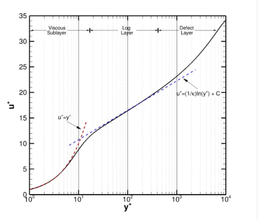
In a wall-bounded flow, the fluid’s motion is restricted by the wall such that the viscous dissipation increases with ever decreasing scales of turbulence dictated by proximity to the wall[16]. It is found that the average shear stress is approximately constant from the wall throughout the boundary layer. This assumption allows for the derivation of the universal law of the wall, which is an empirically-determined description of how the mean streamwise velocity profile of a high Reynolds number turbulent boundary layer behaves near a wall. This velocity profile can be seen in Figure 4. One can see that there are three portions to this profile: the viscous sublayer, the log layer, and the defect layer. However, physically there are only two regions represented here: the inner and outer boundary layer, where the log layer represents the transition between the two[15].

(25)

Figure 4. Typical velocity profile for a turbulent boundary layer.

This plot uses dimensionless parameters for velocity and height that are non-dimensionalized by a velocity scale, which provides a universal relationship such that the profile can be compared between any Reynolds number and boundary layer thick-ness, defined as

uτ ≡

r_τ

w

ρ (2)

where uτ is known as the friction velocity, τw is the wall shear stress, and ρ is the

local density. The dimensionless parameters for velocity,u+_{, and height,}_y+_{, are then}

defined as u+ ≡ u uτ (3) y+ ≡ uτy ν (4)

(26)

whereuis the streamwise velocity,yis the height from the wall, andν is the kinematic viscosity.

It is asserted that near the wall mean streamwise velocity is dependent only upon the wall shear, τw, the distance from the wall, y, and the fluid properties viscosity,

µ, and density, ρ. A dimensional analysis yields the universal law of the wall as presented by Rotta as[16]:

u+ =F1(y+) (5) or ∂u ∂y = uτ y F2(y +₎ ₍₆₎

In the near-wall region the viscosity dominates and thus Equation (5) becomes

u+ =y+ (7)

as shown in Figure 4. Away from the wall the viscosity contributes a negligible amount to the interaction of the mean flow and Reynolds stress carrying eddies and thus F2 is simply a constant, 1/κ, and Equation (6) can be integrated to the law of

the wall presented as

u+ = 1 κlny

+₊_C ₍₈₎

where κ is von Karman’s constant found to be approximately 0.41 and C is an inte-gration constant found to be approximately 5.0 from experiments conducted on flat plates[17].

A van Driest transformation can be applied to the velocity profile to allow com-parison of a compressible flow to the incompressible law of the wall. The van Driest

(27)

transformation is provided by the following integration[18]: u+_vD = Z u+ 0 r ρ ρw du+ (9)

2.2 Hierarchy of Turbulence Modeling

To accurately describe turbulence one would have to use a Direct Numerical Sim-ulation (DNS) in which the entire set of Navier-Stokes equations is solved and the entire set of physics is preserved for the flow. This would dictate the use of a grid that was discretized into elements small enough to resolve the smallest scales of turbulence leading to an extremely high number of grid points and therefore an extremely small allowable timestep. Specifically, the number of grid points needed to sufficiently re-solve the smallest turbulent eddies scales as a function ofRe9/4_{[9][12]. To circumvent}

this issue, turbulence models are used to model the smaller scales, that require smaller grid spacing, in order to create a less-costly computation. The two major classes of turbulence models are Large Eddy Simulations (LES) and Reynolds-Averaged Navier-Stokes (RANS). LES models only the smallest of turbulent scales while fully including the physics of large scales and allows for time-dependent, or unsteady, calculations. RANS, on the other hand takes a temporal average of the entire flow. A helpful graphic depicting the hierarchy of turbulence modeling according to Blazek can be found in Figure 5[4]. In this graphic, Level 0 represents models which solve the full set of Navier-Stokes equations, simply DNS. Level 1 includes methods that model the smallest scales of turbulence, solely LES. Level 2 are second-order closures to include Reynolds-stress models and Level 3 are algebraic closures to RANS which are based on the eddy-viscosity hypothesis of Boussinesq[4].

(28)

Figure 5. Hierarchy of Turbulence Models[4].

2.3 Large Eddy Simulation (LES)

Large Eddy Simulations use the observation that small turbulent structures are more universal in character than large eddies[4] and that the large eddies carry the ma-jority of the Reynolds stress[15]. Therefore, the larger energetic scales are calculated directly while the effects of the smaller energetic scales are modeled[4]. Graphically, one can see the energy spectrum of a turbulent flow in Figure 3 with the scales of the energy spectrum decreasing as the length scales decrease. One can also see

(29)

rep-resentative cutoff points of where certain models begin modeling the smaller scales. These subgrid-scale models allow for a reduction in grid resolution and thus LES can be applied at a Reynolds number an order of magnitude larger than DNS[4].

In boundary layer flows the energetic scales in the inner layer (approximately the inner fifth of the boundary layer) become increasingly smaller as the Reynolds number increases. This creates a ”near-wall problem” in which smaller grid spacing is needed to fully resolve the flow near a wall to a point such that the wall-adjacent cell is under one wall unit (y+≤1)[5]. This increase in grid resolution leads to a need for a num-ber of grid points approaching the cost of Direct Numerical Simulation (DNS)[12], thus limiting the Reynolds number that can be studied and greatly increasing the computational cost of simulations. To perform high Reynolds number LES simula-tions a CFD practitioner has several opsimula-tions, including: running simulasimula-tions on full high-performance computers, running simulations at a fractional Reynolds number, under-resolving simulations, or wall-modeling.

Wall-Modeled LES.

To compensate for the “near-wall problem,” wall-models are introduced which model the energetic eddies in the inner layer while still fully resolving the large-scale eddies found in the outer layer. These models correlate the velocity on the inner boundary of the outer layer to a single value of the wall shear stress[4]. Larsson et al. classify wall-models into two classes: those that use a hybrid LES/RANS method and those that use wall-stress models[12].

In the hybrid LES/RANS model LES computations are used above a certain threshold, between the inner and outer boundary layer, denoted byyint while RANS

is used below. Within hybrid LES/RANS there are two classifications of methods. The first is the models that maintain a fixed yint during grid refinement and thus can

(30)

reach a grid-convergence state since the smallest resolved LES eddies will have a size proportional to yint. The second classification within Hybrid LES/RANS includes

models in which yint is an interface location that is dependent on the grid and/or

solution.[12]

Hybrid LES/RANS captures the large scale movement of energetic eddies unlike the completely RANS model, while using RANS to predict the attached boundary layer, in which it is well suited to do so. Hybrid RANS/LES has been successfully applied to flows such as injector ports and nozzles[19, 20, 21]. The disadvantages are that the energetic frequencies near the wall are lost. These small-scale eddies are critical to the dynamics near the wall and thus a better simulation is needed for resolving the shock turbulent boundary layer interactions of interest in hypersonic flows.

Once again Larsson et al. classifies the other class of wall-models, those that use wall-stress models, into two sub classes: models based on math or physical arguments[12]. The math-based models use control theory and filtering to assert mathematical arguments in order to predict wall stresses or slip velocity such as those of Nicoud et. al and Bose and Moin[22, 23]. The second class of wall-stress models use physics-based arguments, specifically momentum conservation in a nearly parallel shear flow such as those of Balaras et. al, Schumann, and Kawai and Larsson[24, 25, 26]. These physics based models assume either equilibrium, wherein the convection and pressure-gradient terms balance exactly, or non-equilibrium wherein all physics is accounted for[12]. Although Dawson et al. state that an equilibrium model may be insufficient for the flows of interest in this study, it has been shown that using a non-equilibrium model provided a prediction of skin friction that was no more ac-curate than an equilibrium model[27]. Larsson asserts that this is true because the LES itself treats 80% of the boundary layer and thus the wall-model is fed accurate

(31)

instantaneous information that captures the non-equilibrium effects of the flow[12]. Both an equilibrium and non-equilibrium wall-model will be studied in this research. The current challenges of WM-LES are predicting separated and non-equilibirum flows as well as modeling multi-physics effects[12]. Recent successes of using WM-LES for a non-equilibrium flow have been documented by Park and Moin and for separated flow by Shur et. al[28, 29].

2.4 Mathematical Formulation

Navier Stokes.

The fundamental set of equations used for this simulation are the unsteady three-dimensional Stokes equations. Written in divergence law form, the Navier-Stokes equations for one species are

∂U ∂t + ∂F1 ∂x1 +∂F2 ∂x2 +∂F3 ∂x3 = 0 (10)

where U is the vector of conserved variables and Fj is a vector of fluxes in the xj

direction, as given below

U =             ρ ρu1 ρu2 ρu3 E             , F =             ρuj ρu1uj +pδ1j−σ1j ρu2uj +pδ2j−σ2j ρu3uj +pδ3j−σ3j (E+p)uj−σkjuk−qj             (11)

whereinρis the density of the gas, uj is the velocity in thexj direction,pis the static

pressure of the gas,δij is the Kronecker delta,σ is the viscous stress tensor, E is the

(32)

The set of Navier-Stokes equations is closed through the use of an equation of state. For these experiments, a perfect gas is assumed and therefore the ideal gas law, given by equation (12), can be used as the equation of state.

p=ρRT (12)

This equation of state along with the definition of total enthalpy, specific gas constant, R, and ratio of specific heats,γ, allows a relationship for pressure to be written in terms of the primitive variables ρ, ui, and E as given in equation (13).

p= (γ−1)ρ E− uiui 2 (13) For a Newtonian fluid the viscous stress tensor, σ can be defined as

σij = 2ˆµSij +λ

∂uk

∂xk

δij (14)

where Sij is the rate of strain tensor given by[30]

Sij = 1 2 ∂ui ∂xj +∂uj ∂xi (15) and the bulk viscosity, λ, is taken according to Stokes hypothesis that:

λ=−2

3µ (16)

The heat flux vector, qj, is given by Fourier’s Law to be:

qj = ˆκ

∂T ∂xj

(17) The effective viscosity, ˆµ, and effective thermal conductivity, ˆκ, are approximated using the Boussinesq approximation, which assumes a linear relationship between the

(33)

turbulent shear stress and the mean strain rate, therefore

ˆ

µ=µ+µt κˆ=κ+κt (18)

whereµis the molecular component of viscosity,µtis the turbulent component of

vis-cosity, κ is the molecular component of thermal conductivity, andκt is the turbulent

component of thermal conductivity[5].

LES.

Large Eddy Simulations of compressible flows employ the use of both spatial filtering and Favre averaging along with the use of a Sub-Grid-Scale (SGS) model to achieve the aforementioned modeling of small scale turbulent fluctuations.

Spatial Filtering.

The premise of LES is that through the use of filtering the flow can be modeled with any flow variable,U, divided in to a filtered,U, and sub-filter portion,U0 where:

U =U +U0 (19)

The filtered portion is the low-frequency turbulent eddies which are fully resolved while the sub-filter portion are the high-frequency turbulent eddies, which as previ-ously discussed, are universal in character and are therefore modeled. The filtered variable is determined through the use of a low-pass filter with the form

U(#»r0, t) =

Z

U(#»r , t)G(#»r0,#»r ,∆)d#»r (20)

where #»r is the position in space and G is the filter function. The filter function, G, is a function of the difference in space #»r0− #»r and the filter width ∆ defined as

(34)

∆ = (∆1∆2∆3)1/3 where the subscripts denote each spatial direction[4].

The three most well known types of explicit filters are a Tophat, Fourier cut-off, and Gaussian. However, more commonly, filtering is done implicitly through the use of grid spacing along with the inherent discretization error of all calculations.

Favre Averaging.

Favre averaging, or density weighted averaging, is used when the density is not constant, such as compressible flows. This form of averaging provides a simplified set of equations while keeping the non-linear nature of the compressible form of the Navier-Stokes equations. Similarly to before the flow variable,U, is decomposed into a average quantity, ˜U, and fluctuating portion,U00 where:

U = ˜U +U00 (21)

The averaged variable is given by[4]:

˜ U(#»r0, t) = ρU ρ = 1 ρ Z ρ(#»r , t)U(#»r , t)G(#»r0,#»r ,∆)d#»r (22) Wall-Model.

The wall-model developed by Komives will be implemented for this study[5]. This wall-model uses a reduced set of the Reynolds-Averaged Navier-Stokes in the modeled region to account for compressibility, heat transfer, and inertial effects. For the wall model the x1 and x2 directions are arbitrarily assigned orthogonal wall-tangent

directions while x3 is defined as wall-normal. Several key assumptions are made for

the wall-model. First, the pressure in the wall-normal direction is assumed to be constant allowing for the decoupling of the conservation of wall-normal momentum and the conservation of mass from the full Navier-Stokes equation set. From the

(35)

equation of state equation (10) becomes[5] ∂Q ∂t + 1 ρ ∂G1 ∂x1 + ∂G2 ∂x2 = 0 (23) where Q=       u1 u2 e       , Gj =       ρu1uj +pδ1j −σ1j ρu2uj +pδ2j −σ2j (E+p)uj−σkjuk−qj       (24)

In an equilibrium boundary flow it is assumed that the production and dissipation terms balance each other and the sum of the diffusive terms is zero. With these assumptions the equilibrium wall-model omits the convective and pressure gradients. When these assumptions are not made a non-equilibrium model is formed in which these convective and pressure gradients are included, through use of two inertial source terms[5]. In the non-equilibrium model the convective term is pulled from the probe location and Van Driest damping is employed to the wall. The convective term is turned off when there is a strong pressure gradient in the wall-tangential direction. This set of equations is suited for implicit solution and thus the solution strategy of Bond and Blottner is employed, in which the density field and flow primitives are updated in an outer loop while the remaining equations are solved in a decoupled fashion in an inner loop[31]. For further detail on the derivation of the wall-model see Appendix A of Reference [5].

This reduced set of equations is employed on a node-based mesh in the near wall region, where the outermost cell of the wall-model coincides with the probe location in the solver, as can be seen in Figure 6[32].

The probe location is taken to be several cells off the wall, as suggested by Kawai and Larsson, due to the inaccuracy of the first several cells off the wall[26].

(36)

Figure 6. Embedded wall-model grid showing probe location at 4 cells off the wall[5].

Eddy Viscosity Modeling.

The eddy viscosity model used for this wall model is a mixing length model with near-wall damping. This eddy viscosity model is chosen because it describes the eddy viscosity profile typical of the near-wall region of a boundary layer not subject to any pressure gradient, as assumed in the equilibrium wall-model. This method is completely local, requiring only local wall-shear,τw, density,ρ, and distance from the

wall,x3, as given in Equation (25)

µt =ρκx3

r_τ

w

ρ D (25)

with the damping function, D, defined as

D=h1−e−(x∗3/A+)

i2

(26)

where, A+ _{= 17, the von Karman constant,} _{κ, is 0.41, and the wall coordinate,} _x 3 is

(37)

x∗₃ =x3

√

ρτw

µ (27)

Details of the development and basis for Eqs. (25)-(27) are given in reference [5].

2.5 STBLI

Shock Turbulent Boundary Layer Interactions (STBLI) occur when the bound-ary layer separates due to an adverse pressure gradient produced by a shock. These interactions create low-frequency oscillations in the shock position and therefore fluc-tuations in the pressure and density distributions of such a flow over an object of engi-neering interest[2]. Numerous experimental studies have been performed on a wide va-riety of shock turbulent boundary layer interactions, including both two-dimensional and three-dimensional interactions[33, 34, 35, 36, 7]. While a much smaller number of DNS or wall resolved LES has been performed on such flows[37, 38, 39, 40, 41]. Specifically within wall-modeled LES, the studies are largely only for two-dimensional flows[32, 27]. For flows of engineering interest though the flows are more often three-dimensional and thus more information is needed on how these wall-models handle three-dimensional flows such as fins, cylinders, and swept ramps[5]. Adler et al. pro-vides a comparison between computational efforts and experimental results of the STBLI of a swept-compression ramp[2]. The results look promising for two dimen-sions, and the intent of this study will be to assess predictions of wall-models for three-dimensional shock turbulent boundary layer interactions, such as that produced by a swept-compression ramp.

(38)

2.6 Geometry of Interest

The geometry of interest for producing three-dimensional STBLI is a swept-compression ramp with 22.5◦ of compression and 30◦ of sweep. This specific geometry was chosen due to the availability of previous data from the wind-tunnel experiments of Vanstone et al. and the WR-LES of Adler et al.[2, 7]. While both of the aforemen-tioned studies focus on analysis of the unsteady dynamics of the STBLI, the current study will focus more closely on the wall-model’s ability to predict these unsteady phenomena. Further details of the computational and experimental studies will be discussed in Chapter 3.

The interactions seen in the different swept-compression-ramp configurations pos-sess a conical symmetry in which the mean flow properties and frequency content converge to a virtual conic origin (VCO) when plotted in spherical coordinates. This means that the separation length grows linearly with displacement from this VCO, as seen in Figure 7[2].

Figure 7. Diagram of the collapse of separation, ramp corner, triple point, and reat-tachment to the VCO by Adler et al.[2]

(39)

The Virtual Conic Origin (VCO) is expected to be at an x location of −3.4/δ99

and z location of −5.8/δ99, where x is the streamwise direction and z is the spanwise

direction with the origin located at the upstream-ramp-corner[2].

In these three dimensional interactions the flow separation remains open and low-frequency unsteadiness (Stδ ≤ 0.01) is not prominent[2]. Mid-frequency dynamics

(0.01< Stδ <0.2), however, are observed and are related to Kelvin-Helmholtz

(40)

III. Methodology

The general CFD method begins with defining the geometry and flow of interest. This specified domain is then discretized to form a computational grid that covers both the surface and volume of interest. A simulation is then run using this grid and the desired numerics combined with the appropriate boundary conditions for the flow. From this simulation the results are verified and conclusions are drawn about the observed flow characteristics.

3.1 Previous Studies’ Geometry and Flow Conditions

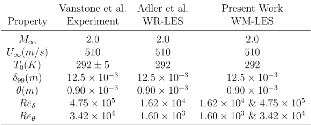
The geometry selected for study, in order to produce a three-dimensional shock turbulent boundary layer interaction, was a swept-ramp with a sweep angle of 30◦ and a compression angle of 22.5◦. This specific ramp was chosen due to the avail-ability of previous results from both experimental studies, of Vanstone et. al, and wall-resolved simulations, of Adler et. al[7, 2]. The aforementioned wall-resolved simulation of Adler et al. used a fractional Reynolds number to make the study tractable. The present study first ran simulations of this fractional Reynolds number in order to determine the wall-model’s capability in predicting aerodynamic quanti-ties as compared to a wall-resolved study. This study also includes simulations at the experimental Reynolds number to determine if large scale features of the interaction were captured in a fashion similarl to the fractional Reynolds number case. A sec-ond reason was to determine the capability of the wall-model in computing a high Reynolds number flow in a relevant amount of time. The flow conditions used for the original experimental study of Vanstone et al., the WR-LES of Adler et al. and the WM-LES of this study are presented in Table 1[7, 2]. All simulations were run using a perfect-gas assumption.

(41)

Table 1. Experimental, WR-LES, and WM-LES flow properties.

Vanstone et al. Adler et al. Present Work

Property Experiment WR-LES WM-LES

M∞ 2.0 2.0 2.0 U∞(m/s) 510 510 510 T0(K) 292±5 292 292 δ99(m) 12.5×10−3 12.5×10−3 12.5×10−3 θ(m) 0.90×10−3 _0.90_×₁₀−3 _0.90_×₁₀−3 Reδ 4.75×105 1.62×104 1.62×104 & 4.75×105 Reθ 3.42×104 1.60×103 1.60×103 & 3.42×104

3.2 Domain and Discretization

Domain.

The domain for this study, despite including a relatively simple geometry, was created in Solidworks 2016, a computer-aided design software, so that precise control of two specific features could be exercised. The first of these two features was at the downstream outflow domain. In order to promote orthogonality at this domain during grid smoothing it is desirable to incorporate a large fillet such that there are no sharp angles initiated by the ramp. The fillet ensures that the gridlines smoothly transition from perpendicular to the ramp to vertical. This fillet was created such that the circle was perpendicular to both the ramp plane and the horizontal top of the domain. The design of this fillet can be seen in Figure 8.

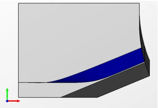
The second of these features was a baffle surface placed approximately four bound-ary layer thicknesses, 4δ, from the ramp wall. This was done so that a convergence study could be easily performed on the boundary layer spacing of the grid by creating a fixed distance that points could be spaced between in the wall-normal direction. A smooth baffle surface was chosen rather than a translated swept-ramp, again, in order to promote orthogonality during grid smoothing. This baffle surface can be seen in Figure 9.

(42)

Figure 8. Diagram of cross-section of domain, in the x-y plane, showing the fillet at the downstream outflow.

The domain started approximately 32 boundary layer thicknesses before the up-stream ramp-corner in the x-direction such that the synthetic turbulent inflow, to be discussed later, had an adequate amount of time to equilibrate before the region of interest occurred. The domain then extends approximately 24 boundary layer thick-nesses past the upstream-ramp corner in the x-direction to allow enough room for the interaction region followed by growth cells for dissipation. The top of the domain was fixed at a height of 0.3125m in the y-direction again to allow enough room for any pertinent interactions to occur along with growth cells for dissipation. The domain was a fixed width of 0.2125m in the spanwise z-direction, matching the wall-resolved study of Adler et. al, and providing adequate room for spanwise relief of the flow.

(43)

Figure 9. Diagram of domain showing the baffle surface 4δ above the wall, as depicted in blue.

Discretization. WM-LES Grid.

To create the meshes used for the wall-modeled simulations Link3D and Pointwise were used conjointly to create block-structured meshes that were orthogonal, low-skew, and isotropic. GoHypersonic Inc.’s Link3D is a parallel-capable multi-block structured grid smoother purposely built for hypersonic research[42], while Pointwise is an all-purpose mesh generation software. As mentioned previously, in order to study grid convergence it was desired to have a fixed spacing between the wall and the baffle surface. To accomplish this a near-wall mesh was created in LINK3D that encompassed the volume from the wall to the baffle surface at 4δ above the wall. This grid was created such that orthogonality was achieved at each of the boundaries, including the baffle surface. The number of points in the wall-normal direction were then simply adjusted to achieve different grid spacing.

(44)

turbulent structures in those respective directions, using the WR-LES grid of Adler et al. as an estimate of the number of cells needed[2]. These grid spacings also align with the best practices of the LES community, as prescribed by Georgiadis et. al, in which[43]:

50≤∆x+ ≤150 15≤∆z+ ≤40 (28)

with x as the streamwise direction and z as the spanwise direction. The values for this study are presented in Table 2.

Table 2. Grid spacing of WR-LES

Reδ ∆x+ ∆z+

1.62×104 ₄₉ ₂₈

To ensure grid independence, a grid with one-half the number of cells on the wall, and approximately 70% of the number of points in both the spanwise and streamwise direction, was created. The grid spacing in the streamwise direction was chosen such that equal spacing was achieved at the spanwise center of the grid, since the sweep of the ramp creates a difference in spacing on either side. Grid stretching was applied near the outflow in order to provide dissipation of any numerical errors that could be reflected back into the region of interest (the ramp corner).

The grid was then finished in Pointwise where hyperbolic tangent stretching was applied from 4δ to the top of the domain. The spacing of the first cell along the baffle in the wall-normal direction was chosen to match the fixed spacing within the lower region such that there was a smooth transition between the two blocks. The number of points in the wall-normal direction was fixed in this region creating slightly different grid stretching in this upper block between grids. Grid stretching was also applied near the top of the domain since it primarily consists of freestream properties

(45)

with no flow of interest as well as to dissipate any unphysical flow phenomena from returning to the region of interest. A cross-sectional view of one of these grids can be seen in Figure 10. Of note is that the same grid was used for both the wall-resolved Reynolds number cases and the experimental Reynolds number cases.

(a) Domain beginning at 20δ,

display-ing every 10th grid line (b) Focus on ramp-corner

Figure 10. Cross-section of surface grid used in the WM-LES studies.

Table 3. Grid Properties for wall-normal grid convergence study.

Grid Lx Ly Lz ∆x ∆y ∆z ∆x+ ∆y+ ∆z+ Ntotal

Coarse 52δ99 25δ99 17δ99 δ99/20 δ99/30 δ99/32.5 49 60 28 107M

Medium 52δ99 25δ99 17δ99 δ99/20 δ99/40 δ99/32.5 49 50 28 129M

Fine 52δ99 25δ99 17δ99 δ99/20 δ99/50 δ99/32.5 49 40 28 151M

The total number of cells, Ntotal, is not a good comparison between the WR-LES

and WM-LES grid size since different synthetic turbulence methods were used causing differences in the length of the inflow region. However, for the same spanwise and streamwise grid spacing as the WR-LES the WM-LES coarse, medium, and fine grids provided a 36%, 20%, and 4% reduction in wall-normal grid points, respectively.

(46)

DDES Grid.

Wall-resolved grids with wall-normal spacing under one wall unit (y+ _≤ _{1) were}

also created for use in Delayed Detached Eddy Simulation (DDES). Unlike before, two different grids were created for each of the Reynolds numbers to achieve the aforementioned condition at the wall. These grids were created entirely in Link3D with spanwise and streamwise spacing being the same as the wall-modeled grids but with grid clustering now in the wall-normal direction. The near-wall spacing was selected as to achieve a y+ _{= 1 based on that grid’s specified Reynolds number and}

a growth rate of 8% was applied away from the wall. The same grid stretching was applied near the downstream outflow and top of the domain A cross-sectional view of one of these grids can be seen in Figure 11.

(a) Domain beginning at 20δ (b) Focus on ramp-corner

Figure 11. Cross-section of surface grid used in the DDES studies.

3.3 Boundary Conditions

The wall boundary condition was chosen to match the experiment with an isother-mal condition set at a fixed stagnation temperature provided from the experiment of

(47)

292K. The outflow and the ceiling of the test volume were set as supersonic outflows and the upstream-ramp-corner side was set as an adiabatic no-slip wall to simulate the placement of a fence within the experiment[2]. The downstream-ramp-corner boundary condition was originally selected to be a supersonic outflow; however, this led to increased separation due to the presence of spanwise reverse flow caused by the swept ramp. To fix this issue, a hybrid boundary condition was used as done by Adler et al.[2]. Any flow at the boundary with a positive spanwise velocity was treated with a supersonic outflow condition as before, but any flow with a negative spanwise velocity, thus an inflow, was treated with an adiabatic slip wall condition in which the spanwise velocity becomes zero. Finally, the inflow was treated with an artificial turbulent inflow. A diagram of the prescribed boundary conditions is found in Figure 12.

Figure 12. Boundary Conditions with x-y cross-section on the left and top down, x-z cross section on the right.

Turbulent Inflow.

To create the artificial turbulent inflow, the digital filtering technique of Kartha et. al was used[44]. In this method a two-dimensional RANS simulation of a flat-plate at the flow conditions of interest was first run. From this simulation, the streamwise position of the desired boundary layer thickness was found. A one-dimensional

(48)

bound-ary layer profile was then taken from a distance 30δupstream from this location such that the inflow provides a boundary layer height that grows to the desired thickness near the separation. Inflow pertubatons of this profile were generated as to provide a time varying inflow with appropriate Reynolds stresses weighted for compressibility by the use of Morkovin scaling[5]. Both the normal and shear Reynolds stresses along the flat-plate portion of the domain were compared to the incompressible profile of DeGraaff and Eaton to determine whether the synthetically generated turbulence was equilibrated[6].

3.4 US3D

The analysis software used for this study was US3D version 1.0RC22, a finite-volume compressible Navier-Stokes solver extensively validated for hypersonic flows[45]. The numerical methods chosen for these studies, available in this tool, are discussed below.

LES.

For the LES simulations time advancement was done using 3rd Order Runge-Kutta time integration. Inviscid fluxes were evaluated using the kinetic-energy consistent scheme of Subbareddy and Candler at 2nd order for one flow time, to help initialize the flow from a free-stream with artificial boundary layer initial condition, before being increased to 6th order for the remainder of the simulation[46]. A Ducros sensor was used as a shock sensor. The Vreman model was used for subgrid-scale viscosity in the LES due to its availability in the software[47]. For wall-modeled cases the wall-model of Komives was used to provide corrected wall heat flux and skin friction to the LES calculation as detailed in Section 2.4[5].

(49)

times in order to initialize the turbulence needed for the wall-model assumptions. Once the wall-model was turned on the simulations were run for four flow times before mean statistics were collected for four flow times. Although this provided solutions in some variables that are visibly not converged, the statistics are deemed indicative enough to draw conclusions from.

DDES.

For the DDES simulations, 2nd order implicit Crank-Nicolson time integration with point relaxation was used. Inviscid fluxes were evaluated at 2nd order for one flow time as with the LES, but 4th order after that. Turbulence was modeled using Delayed Detached Eddy Simulation with the original Spalart-Allmaras model (SA-Catris)[13, 14].

3.5 Test Matrix

Grid Convergence.

Normally, to show grid convergence one must show that the results produced are independent of the grid. In the case of WM-LES there are two grids for which this must be proven true; the large scale LES grid as a whole and the one dimensional wall-model grid.

LES Grid.

As discussed previously the grid in the area of interest, approximately 4δ from the wall, has fixed spacing in the wall normal direction. To show grid convergence this spacing was varied with respect to the number of cells per boundary layer. Grids with wall normal spacing of δ/30, δ/40, and δ/50 were used. Special care was used to ensure that the wall-model physical probe location stayed at approximately the

(50)

same location when pulling from each of these grids. A grid with one half the number of cells on the wall was also run to ensure grid independence in the streamwise and spanwise directions.

Wall-Model Grid.

With the location of the wall-model probe fixed, the density of the one-dimensional wall-model grid was varied to ensure grid independence within the wall-model. The medium density grid was run using three different numbers of wall-model points: 17, 35, and 60. The intermediate number of points, 35, leads to a wall-model z+ _{of 1}

for the first point in the wall-model and a wall-model z+ _{within the log-layer at the}

probe location.

Wall-Model Flux Changes and DDES.

A DDES simulation was run at both the experimental and wall-resolved Reynolds numbers for use in comparing how other methods of handling high Reynolds numbers flows do in comparing the same interaction. The wall-modeled calculations were run using the medium density grid for three different flux schemes: an equilibrium model, one with the added pressure term, and one with convective fluxes added.

3.6 Comparisons

Comparisons were drawn between the wall-modeled LES and both the wall-resolved study of Adler et al. and the experiment of Vanstone et al.. Comparisons were also made to simulations run using Delayed Detached Eddy Simulation (DDES) using the Catris-Aupoix compressible formulation of the Spalart-Allmaras one-equation turbu-lence model[13][14].

(51)

surface statistic line plots at several locations across the span to include lines at: 2δ, 4δ, and 8δ from the fence side. Comparisons of mean primitive variable contours were done at 4δ from the fence side. Surface streamlines plots were also compared for location of the VCO and finally power spectral density surrounding the interaction region was compared.

The same mean primitive variable contour plots were compared to particle image velocimetry (PIV) from the experiments. Surface streamlines were also compared to the oil flow visualization of the experiment.

Mean surface statistic line plots were used to compare values of aerodynamic properties to the DDES results. Once again, the surface streamlines were used to determine the location of the VCO. Conclusions were drawn on the ability of the wall-model to predict both aerodynamic quantities and the location of large scale interaction features.

(52)

IV. Results and Analysis

Before reporting the results of a Large Eddy Simulation, it is first important to show the computation’s sensitivity to certain modeling parameters such as grid density, grid stretching, and boundary conditions[43]. For this study the sensitivity to grid density of the LES grid as well as the one-dimensional wall-model grid will be studied. The quality of the incoming turbulent statistics from the inflow boundary condition will be validated, the adiabatic wall temperature will be verified, and finally the appropriateness of the wall-model probe location will be determined.

4.1 Grid Independence Results

LES Grid.

To begin, the sensitivity of the LES grid to cell density was studied. Two different studies were completed; one combining the streamwise and spanwise directions along with one in the wall-normal direction. To determine the sensitivity of the solution to different grids, mean surface quantities, to include the three-directions of wall-shear and pressure, were compared at the midspan, approximately 8δ from the upstream ramp-corner side as shown by the line in Figure 13. When plotting data along this line the streamwise coordinate is normalized by the incoming boundary layer thickness (δ = 12.5×10−3_{), with} _x/δ _{= 0,} _y/δ _{= 0,} _z/δ _{= 0 located at the}

upstream-ramp-corner.

Three LES grids were studied each with different wall-normal spacings between the ramp wall and a baffle surface approximately 4δfrom the ramp wall. The coarsest of the grids had wall-normal spacing of δ/30 which led to a y+ _{between 70 and 150}

across the wall. The medium density grid had wall-normal spacing ofδ/40 which led to a y+ _{between 50 and 130. And, the finest of the grids had wall-normal spacing}

(53)

Figure 13. Depiction of locations where the mean surface quantities are extracted from. Contour colors are of skin friction coefficient for a WM-LES simulation.

of δ/50 which led to a y+ _{between 20 and 120. The lower values occurred within}

the separation region and the flat-plate portion of the domain while the larger values occurred post-reattachment.

The results of this grid convergence study can be seen in Figure 14. One can see that while the δ/40 and δ/50 grids agree well the coarsest of the grids, δ/30, varies more. The largest difference in values of shear in the x-coordinate is in the flat-plate portion of the domain where approximately a 2% difference between the fine and medium grids is seen while close to a 10% difference is seen between the coarse and fine grids. In the y-coordinate the greatest difference is seen in the minimum just after the ramp-corner. Between the fine and medium grids there is less than a 1% difference while between the coarse and fine grids there is a 30% difference. The

(54)

spanwise, z-direction, shear converges much slower than the other directions, and thus it is hard to determine the exact difference among the three. However, the coarsest grid does seem to predict values of τz lower than the medium and fine. The pressure

is predicted the most closely among the three grids with less than a 1% difference between the fine, medium, and coarse grids. Since the δ/40 and δ/50 grids have a functionally insignificant difference in solutions the coarser of the two grids,δ/40, was chosen for use in the rest of the simulations for computational efficiency.

(a) x-direction wall shear (b) y-direction wall shear

(c) z-direction wall shear (d) pressure normalized by freestream

(55)

After the computations sensitivity to wall-normal spacing had been determined the grid independence of the streamwise, x-coordinate, and spanwise, z-coordinate, spacing was verified. As mentioned previously the initial streamwise and spanwise spacings were chosen based on the wall-resolved study of Adler et al. as well as the suggested spacings of Georgiadis et al.[2, 43]. The results of this original grid spacing compared to a case with half the number of points on the wall, or approximately 70% of the points in each direction, can be seen in Figure 15.

Figure 15. Spanwise and streamwise grid convergence study mean surface quantities: z = 8δ

(56)

Despite looking similar in profile there is a large difference between the two sim-ulations. In the x-direction, the drop in shear occurs more rapidly and thus at ap-proximately x/δ = −3.0 there is a 35% difference in the value of x-direction wall shear. Similarly to the wall-normal convergence study, the largest difference in the y-direction wall shear occurs just after the ramp-corner. Between the full resolution grid and the half resolution grid there is a 32% difference in the minimum value. Again, due to slow convergence, it is tough to determine the exact difference of the z-direction shear between the two simulations but the half resolution grid does tend to be below that of the full resolution gird. And finally, the pressure values once again are very close with less than a 1% difference between the full and half resolution grids. Due to the large differences in predicted shears the full resolution grid is chosen for use in the remainder of the studies.

Wall-Model Grid.

With the determination that the medium density LES grid, δ/40, with the span-wise and streamspan-wise spacing of the wall-resolved study of Adler et al. is sufficiently resolved the sensitivity of the computation to the one-dimensional wall-model grid must be determined. Three different wall-model grid densities were used in simula-tions; one with 35 points which provided a wall-model y+ ≈ 1.0, one with half the number of points (17) which led to ay+≈2.5, and one with slightly less than double the number of points (60) which led to ay+ ≈0.6. The results of the wall-model grid convergence study are found in Figure 16.

One can see that all the solutions match very closely, especially within the region of interest from approximately 5δ to 10δ. The only discrepancy among the three is that the highest resolution wall-model, with 60 points, varies near the outflow in the three wall shear directions. Since this region is not of interest and the difference is

(57)

Figure 16. One-dimensional wall-model grid convergence study mean surface quantities: z = 8δ

less than 20% at its largest the wall-models are deemed to be converged. The medium density wall-model grid, with 35 points, was chosen for use such that we maintain the desired condition that y+ ≤1.0 while not adding extra computational burden by adding additional points and thus calculations.

(58)

4.2 Wall-Model Probe Location

In addition to verifying that the one-dimensional wall-model has appropriate reso-lution one must also verify that the underlying assumption that the wall-model probe is placed within the log-layer is met. To do this, the dimensionless wall distance and van Driest transformed dimensionless velocity were extracted from the flow along the midspan 30δ from the inflow, a point just before the separation region, and plotted as seen in Figure 17. The wall-model probe for this particular simulation was placed four cells from the wall as identified in Figure 17 by the circle. During simulations the y+ _{of the probe location was recorded at each iteration and was found to match}

this point of approximatelyy+_{= 5.6}_×₁₀2_{. Since this point does appear to fall within}

the log-layer, approximately y+ _≤₁₀3 _{for this location, it is deemed that this probe}

location fulfills the assumption of the wall-model.

4.3 Boundary Conditions

To assess the quality of the incoming turbulent statistics from the inflow bound-ary condition discussed previously the Reynolds shear and normal stresses in the pre-separation boundary layer were studied. A point along the midspan 30δ from the inflow was chosen for study and the Reynolds stresses were compared to the in-compressible profile of DeGraaff and Eaton, with Markovin scaling for compressibility effects, in Figure 18[6] . The wall-normal and wall-tangential Reynolds normal stresses are predicted appropriately with no more than a 5% difference in the wall-tangential stress and very close prediction of the wall-normal stress before y/δ = 0.4 of the wall. The discrepancy between the wall-normal stress aftery/δ = 0.4 is attributed to a compressible boundary layer being compared to an incompressible profile and the existence of the defect layer in this region. The Reynolds shear stress is also predicted

(59)

Figure 17. Log Layer matching of the LES grid with wall-model probe identified. The von Karman constant, κ, is 0.41 and the integration constant, C, is 5.1.

than a 10% difference in the near-wall region and less than 1% after that. With good agreement between these stress profiles, it can be asserted that the turbulence just upstream of the separation region is appropriately equilibrated and thus the synthetic turbulent inflow is suitable.

Another boundary condition of interest is the isothermal wall condition in which the adiabatic wall temperature was set. To check that this set temperature does produce an adiabatic wall the wall heating (from wall to fluid) can be seen in Figure 19. One can see that very small magnitudes, less than 1.0, are found indicating that this is an approximately adiabatic wall temperature, and appropriate for the study.

Now that several simulation factors such as grid density and the turbulent inflow have been validated for adequacy one can compare the simulations to the wall-resolved

(60)

(a) Normal (b) Shear

Figure 18. Reynolds Stresses compared to incompressible profile of DeGraaff and Eaton[6].

and experimental studies with confidence that underlying errors are not creating any of the noted differences.

4.4 Equilibrium Wall-Model

Initially, an equilibrium wall-model was used based on the assertion by Larsson that a non-equilibrium model provided results that were no more accurate than a non-equilibirum model as discussed in Section 2.3[12]. The equilibrium model was first simulated at the Reynolds number of the wall resolved study of Adler et al. as to determine how a simulation with the assumptions of the wall model compares to a simulation which is not modeled at the wall, and therefore hypothetically the best that the wall-model could achieve in predicting the solution.

Virtual Conic Origin - Wall Resolved LES Reynolds Number.

When initially looking at the solution of the modeled simulation at the wall-resolved Reynolds number one can qualitatively tell that there is differences in the

(61)

x/d |q w | (W /c m 2 ) -10 0 10 20 0 0.2 0.4 0.6 0.8 1 δ/40

Figure 19. Wall heating of δ/40 WM-LES case

mean statistics when compared to the wall-resolved study of Adler et al.. These dif-ferences are especially clear when looking at surface streamtraces. The mean surface skin friction coefficient on the wall is displayed with these surface streamtraces in Figure 22. An obvious difference in the surface streamlines is noted with no stream-wise reverse flow in the wall-modeled simulation. This lack of reverse flow allows for the separation front to move forward thus producing a different virtual conic than in the wall-resolved study. The wall-resolved study documented a virtual conic origin (VCO) at −3.4δ,−5.8δ in the x-z plane while the wall-modeled simulation produced a VCO at 0.79δ,1.53δ. The virtual conic of the wall-modeled solution is visualized in Figure 21.

(62)

(a) Wall-Modeled LES (dashed line is ramp-corner)

(b) Wall-Resolved LES

Figure 20. Comparison of surface streamlines between WM-LES and WR-LES (z is up)[2].

Virtual Conic Origin - Experimental Reynolds Number.

The wall-modeled location of the virtual conic origin was also evaluated at the experimental Reynolds number. A similar result occurred with no streamwise reverse flow leading to a VCO at a location of 0.46δ,0.97δ in the x-z plane. The WM-LES