The Split tree for option pricing

(1)

FACHBEREICH MATHEMATIK AG Finanzmathematik

The Split tree for option pricing

Merima NURKANOVI ´C

Supervised by Prof. Dr. Ralf KORN

1. Gutachter: Prof. Dr. Ralf KORN Technische Universität Kaiserslautern 2. Gutachter: Assoc. Prof. Dr. Ömür U ˘GUR

Middle East Technical University, Ankara

Datum der Disputation: 23.05.2017

Vom Fachbereich Mathematik der Technischen Universit¨at Kaiserslautern zur Verleihung des akademischen Grades Doktor der Naturwissenschaften (Doctor rerum naturalium, Dr. rer. nat.) genehmigte Dissertation.

(2)

(3)

Acknowledgement

I would like to express my deepest gratitude to my supervisor Prof. Dr. Ralf Korn for his patient guidance, enthusiastic encouragement and useful critiques of this research work. Without his advices and the valuable discussions, this thesis would have never been written.

I would also like to express my gratitude to Assoc. Prof. Dr. ¨Om¨ur U˘gur who took time to read and review this dissertation.

I sincerely thank my friends, particularly B¨u¸sra, Sema, Andreas and Christoph for the time they took to proof-read this dissertation, and to Luc for his help with pictures. It is with their help that I managed to finish on time.

I would like to thank my colleagues in the Financial Mathemtics group and GRK1932 for their valuable support and the excellent working environment they provided. I am also thankful to these groups for the financial support.

Special thanks to Prof. Dr. Mark Joshi, who invited me to University of Mel-bourne and gave me an opportunity to work with him, Prof. Dr. Kenneth Palmer and Assoc. Prof. Dr. Guillaume Leduc. I am particularly thankful to Assoc. Prof. Dr. Guillaume Leduc for bringing his work on flexible binomial tree to my mind.

Last but not least, I would also like to thank to my lovely parents and sister for their unconditional love and support during all these years. Without them this would be impossible. I am especially grateful to my fianc´e Irvin Hot for his love and help. Without his help with Matlab this thesis would not look the same.

(4)

(5)

(6)

(7)

vii

Abstract

In this dissertation convergence of binomial trees for option pricing is investi-gated. The focus is on American and European put and call options. For that purpose variations of the binomial tree model are reviewed.

In the first part of the thesis we examine the convergence behavior of the already known trees from the literature (CRR, RB, Tian and CP) for the European op-tions. The CRR and the RB tree suffer from irregular convergence, so our first aim is to find a way to get the smooth convergence. We first show what causes these oscillations. That will also help us to improve the rate of convergence. As a result we introduce the Tian and the CP tree and we prove that the order of convergence for these trees is O 1_n

.

Afterwards we introduce the Split tree and explain its properties. We prove the convergence of it and we derive an explicit first order error formula. In our set-ting, the splitting time tk = k∆t is not fixed, i.e. it can be any time between 0

and the maturity timeT. This is the main difference compared to the model from the literature. Namely, we show that the good properties of the CRR tree when S0 =K can be preserved even without this condition (which is mainly the case). We achieved the convergence of O

n−32

and we typically get better results if we split our tree later.

In addition, we examine the behavior of the split tree when applied to American options. This will require some modifications - depending on the initial stock price and the type of option - to take care for the early exercise feature of American options.

(8)

(9)

ix

Abstract (Deutsch)

In dieser Dissertation wird die Konvergenz von Binomialb¨aumen zur Optionsbew-ertung untersucht. Der Schwerpunkt liegt auf Amerikanischen und Europ¨aischen Put und Call Optionen. Zu diesem Zweck werden Variationen des Binomialbaum-modells besprochen.

Im ersten Teil dieser Arbeit untersuchen wir das Konvergenzverhalten von Bi-nomialbäumen für Europäische Optionen aus der einschlägigen Literatur (CRR, RB, Tian und CP). Da die CRR und RB Bäume Oszillationen im Konvergen-zverhalten aufweisen, ist unser erstes Ziel das Auffinden von Möglichkeiten, um glatte Konvergenz zu erreichen. Dazu untersuchen wir zunächst die Ursachen für diese Oszillationen, was uns letztlich zu einer Verbesserung der Konvergenzrate führt. In der Folge stellen wir die Tian und CP Bäume vor und beweisen, dass die Konvergenzordnung für diese Bäume O(1

n) ist.

Im Anschluss führen wir die sogenannten Split-Bäume ein und erläutern ihre Eigenschaften. Wir zeigen, dass diese Bäume konvergieren und leiten explizite Fehlerformeln erster Ordnung her. In unserem Setting ist die Trennungszeit tk =k∆t nicht fixiert, d.h. sie kann frei zwischen dem Startzeitpunkt 0 und der

LaufzeitT gewählt werden. Dies ist der wesentliche Unterschied im Vergleich zur existierenden Literatur. Wir zeigen, dass die positiven Konvergenzeigenschaften der CRR Bäume im Fall S0 = K (was in der Praxis typischerweise nicht der Fall ist) erhalten bleiben, selbst wenn diese Bedingung nicht erfüllt ist. Wir erzielen eine Konvergenzordnung von O(n−32) und zeigen auf, dass ein später

Trennungszeitpunkt f¨ur unsere Binomialb¨aume bessere Resultate liefert.

In einem weiteren Kapitel untersuchen wir das Verhalten des Split-Baums bei der Bewertung amerikanischer Optionen. Hierzu erweist es sich als zweckmäßig -in Abhängigkeit vom Startwert des Aktienpreises und des Typs der Option-, das Verfahren so zu modifizieren, dass der Möglichkeit der vorzeitigen Ausübung bei amerikanischen Optionen Rechnung getragen wird.

(10)

(11)

xi

Chapter 1 Introduction

In the last decades derivatives have become increasingly important in the world of finance. Trading call options started in the Chicago Board Options Exchange in 1973 (CBOE). Options had also been traded earlier but CBOE created an orderly market with well - defined contracts. Trading put options started in 1977 and today many other exchanges throughout the world trade options. The first completely satisfactory equilibrium option pricing model has been introduced by F. Black and M. Scholes [5]. R.C. Merton [32] extended their model in several important ways in the same year. They made a basis for many subsequent aca-demic studies. Their studies have shown that option pricing theory is relevant to almost every area of finance. Unfortunately, Black - Scholes and Merton articles are quite advanced. Luckily, W.F. Sharpe derived the same results using only elementary mathematics.

The binomial approach to option pricing grew out of a discussion between M. Ru-binstein and W.F. Sharpe at a conference in Ein Borek, Israel. They suggested the following principle: if an economy with three securities can only attain two future states, one such security will be redundant. In other words, each single security can be replicated by the other two, a fact later known as market com-pleteness. This observation lead them to a two-state model, but it should be verified that the economic properties of the Black-Scholes diffusion approach are preserved. This was the birth of the binomial option pricing.

Applying binomial trees is a useful and very popular technique for pricing an op-tion, since it is easy to implement. It was introduced by J.C. Cox, S.A. Ross and M. Rubinstein in [9] and R.J. Redleman and B.J. Bartter in [40] independently. A binomial tree can be identified with a diagram that represents all different possible paths that might be followed by a stock price over the life of the option. One of the advantages of the binomial tree is that it can be adapted to options with different types of payoff structure, including American options. Since there is no closed form solution for the price of American options, this is an advantage

(14)

of the binomial trees.

The binomial approach is based on the concept of the weak convergence. We construct the discrete - time model S(n) _{so that convergence in distribution to} the continuous processS is ensured. This means that the expectations calculated in the binomial tree can be used as approximations of the option prices in the continuous models, at least for bounded option payoffs (and with further con-siderations for more general payoffs). Unfortunately, the models defined by J.C. Cox, S.A. Ross and M. Rubinstein (short CRR) and by R.J. Redleman and B.J. Bartter (short RB) have a slow convergence which also is often highly irregular. This motivated other scientists to modify binomial trees suitably to obtain an improved convergence.

Developments of the tree methods can be categorized into three groups. The first group is ”Modifications of conditions on parameters”. Namely, CRR and RB specified the moment-matching conditions so that the moments of the bino-mial tree converge to those of the continuous process when the number of steps used for the discretization goes to infinity (in the CRR tree the first moment is matched exactly and the second only asymptotically, while for RB both are matched exactly). The construction of the new trees differ mainly in the dis-cretization process used, the number of moments to be matched and the way it is done as well as wheter to impose symmetry on the tree or not. Some important trees from this category are suggested by R. Jarrow and A. Rudd in [16]. They discretized the log risk-neutral stock process and imposed symmetry on the move-ment probabilities. Tian in [46] suggested to match the first three raw momove-ments exactly in spot space. More about trees from this category can be found in [20], p.425.

The second group is ”Design of trees with special features”. The main focus of this thesis is on this category. Tian in [47] introduced a tilt parameter into the model. The idea is to tilt a tree so that a node in the tree coincides with the strike price at the maturity of the option. As a result, we get a smooth con-vergence which allows us to additionally use extrapolation methods. Chang and Palmer in [7] (short CP) proposed a similar idea. They constructed the tree so that the strike is at the geometric average of two nodes, i.e. the midpoint of two nodes in log-space. Leisen and Reimer in [31] first specified the movement probabilities in the bond measure and the stock measure and then from there they determined the movement sizes. In addition, the tree was constructed such that the strike is at the center of the tree. Joshi [19] proved that Leisen and Reimer’s tree has a second order convergence. Joshi in [18] introduced the Split tree. The idea of this tree is to have the tree centered around the strike value in log scale. To achieve this, a time depended drift is introduced for the first k

(15)

steps of the tree and afterwards, when we are already in desired position, there is no drift, i.e. we continue with a CRR tree for the rest of the steps. In this paperk is fixed to bek =bn

2c. The main novel result of this thesis is to prove the convergence of the Split tree and to see what is happening if we choose anotherk. The third group is the ”Introduction of acceleration techniques”. Hull and White in [15] applied the ”Control Variate” technique to the binomial trees. The idea is to use European options as a control to American options, so the American option price is adjusted by the error we get by pricing European options. Broadie and Detemple in [6] introduced the so called ”Smoothing” technique. The idea is to replace the continuation value one time step before the maturity with the Black - Scholes price. The motivation is that the Black - Scholes price has a con-tinuous derivative, while the continuation value does not. As a result, the price converges with much fewer oscillations and more smoothly. In the same paper they also used Richardson extrapolation. This helps with removing the error.

Outline of the thesis

Chapter 2 contains an introduction to binomial trees. We gave definitions of some basic type of options and the weak convergence is introduced. Afterwards some properties of the binomial trees are explained and we introduced CRR and RB tree.

In Chapter 3 we discussed more about properties of the CRR tree. We prove that this model has a good performance if we have S0 =K. Afterwards we state and prove the Main theorem. This theorem (Theorem 6) gives the order of conver-gence of the binomial trees for the digital and European call options, but also it gives the error term. These results motivated the introduction of the Tian and the CP tree. These two models achieve a convergence of O 1

n

Chapter 4 is the central part of our work. First, we introduce the Split tree and explain its properties. Afterwards, we prove the convergence of it and we found an explicit first order error formula (helpful discussions on this topic with G. Leduc have been very much appreciated). In our setting, the splitting time tk = k∆t

is not fixed, i.e. it can be any time between 0 and the maturity time T. This is the main difference compared to the model suggested by Joshi. Namely, we show that the good properties of the CRR tree when S0 = K can be preserved even without this condition (which is mainly the case). We achieved the convergence of O

n−32

and we typically get better results if we split our tree later.

(16)

Khanna and we perform a numerical analysis. Different situations are observed and we compare all introduced models. Some discussion about drift in general is presented here, which might help for further research for American options.

(17)

5

Chapter 2 Introduction to binomial trees

Derivatives have become very important in the world of finance over the last decades. In many stock exchanges all over the world options are traded actively. Consequently, there is a market request for mathematical models to price them which makes pricing options one of the most important problems in applied math-ematics. In this chapter we present some types of options, the fundamental Black - Scholes formula for pricing European call and put options, and theoretical and practical aspects of binomial trees as numerical method for option pricing.

2.1 Option types

A derivative is a financial instrument whose value depends on the values of other financial instruments (or derives from), its underlying assets. An option is a simple financial derivative. For example, a stock option is a derivative whose value depends on the price of a stock. There exist also options on equity, foreign currencies, bonds, goods as oil, gold, etc. There exist two basic types of so-called vanilla options.

Definition 1. A call option is a contract which gives its holder the right (but not the obligation) to buy a certain fixed amount of the underlying asset for an already agreed price on or before a certain date. A put option is the contract which gives its holder the right (but not the obligation) to sell a certain fixed amount of the underlying asset for an already agreed price on or before a certain date.

An option is not binding, i.e. the holder is not obligated to buy or sell, which gives rise to the term ”option”. There exist three important groups of options:

• European options, • American options,

(18)

• Exotic options (barrier options, Asian options, Bermudan options, etc). In this thesis the focus will be on European and American options. The name is not connected with the geographical position of the holder, but on the way the option can be used. European options can be exercised only on a certain date, the exercise date (or maturity time). American options can be exercised at any time between now and the maturity time. We denote the maturity time by T. If T is +∞ the option is called perpetual.

European call option

Let us assume that a holder wants to buy a European call on one share of a stock. This means that the holder has the right to buy this share at time t=T for the strike priceK, which is known at the beginning of the contract, i.e. at timet= 0. Let S(T) be the share price at maturity. If S(T)> K, the holder of the option buys the share for the price K and he can sell it immediately at the market for the price S(T). His gain will be S(T)−K. If S(T) < K, the rational holder will decide not to exercise the option. As a consequence, there is no gain from holding the option. Combining these two cases, we get that the final payment of

V(S) = (S(T)−K)+ _{= max{S(T}₎₋_K,_0}. This is also presented in the Figure 2.1.

S(T) 10 20 30 40 V(S) −5 10 20 0

Figure 2.1: Payoff of a European call option with strike price K = 20 Example 1. Let us say we have the situation where an investor buys a European call option with a strike price of $60 to purchase 100 shares of some company. The current stock price is $58, the expiration date of the option is one year and the price of an option to purchase one share is $5. Since we have 100 shares, the initial investment is $500. If the stock price, after one year, is less than $60, the investor will choose not to exercise, since there is no point in buying a share

(19)

2.1. Option types

for $60 which value is less than $60. In this case the investor will lose the initial investment of $500. If the stock price is above $60, the investor will decide to exercise the option. Let us assume that the option price is $70. By exercising the option, the investor will buy 100 shares for $60 per share. If she sells the shares immediately, she will gain $10 per share, i.e. $1000, ignoring transaction costs. After taking the initial costs into account, the investor is left with a net profit of

$500. Nevertheless, it is possible to make a loss. Assume that the value of the company’s option at the maturity is$63. After exercising the option, the investor would gain 100×($63−$60) = $300 and taking initial costs into account, she is left with −$200. However, without exercising she would lose $500, which is a bigger loss than$200. We can conclude that call option should always be exercised at the expiration date if the stock price is above the strike price.

European put option

The holder of a European put has the right to sell one share of a stock at maturity time T for the strike price K. Now we have that in case when K > S(T) the holder will decide to sell the share for price K. On the other hand, if K < S(T) the holder will decide not to exercise the option. Combining these two cases, we get that the final payment is

V(S) = (K −S(T))+_{= max{K}₋_S(T_),_0}.

There is also a case for the put option where the loss can occur, similar to the call option. Payoff of the European put option is also presented in Figure 2.2.

S(T) 10 20 30 40 V(S) −5 10 20 0

Figure 2.2: Payoff of a European put option with strike price K = 20

American options

There exist also American put and call options. As we have seen, European calls and puts can be exercised only at the maturity time T. American puts and calls

(20)

can be exercised at any time between 0 and time T. A closed-form solution of American options is hardly ever available, therefore the usage of the numerical methods is of great importance. In Chapter 6 we will see how to apply binomial trees to calculate prices of American options numerically.

Exotic options

Put and call options are also known as plain vanilla options. An exotic option is an option which differs from a common American or European option in terms of the underlying asset or when and how the investor receives a certain payoff. We will present Asian and Barrier options as an example of exotic options. Asian options

An Asian option is a path dependent exotic option. The payoff of an Asian op-tion depends on the average price of the underlying asset over a certain period of time. An Asian option can protect the investor from short term market ”ma-nipulations”, which can occur close to maturity. We have Asian call options with payoff (S−K)+_{and Asian put option with payoff (K}_−S)+_{, where}_S_{is an average} price over time period [0, T]. Average in continuous time is obtained by:

S= 1 T

Z T 0

S(t)dt.

For the discrete case, with sample points t1, t2, ..., tn, we consider arithmetic and

geometric average: S = 1 n n X i=1 S(ti) S= n Y i=1 S(ti) !_n1 . Barrier options

Another example of path dependent options are barrier options. A barrier option is an option where the payoff depends on whether the path of the underlying asset has reached some pre-specified barrier B during the life time of the contract. There are two main types of barrier options: knock-out and knock-in barrier options.

(21)

2.2. The stock price model (S(T)−K)+_·₁ max t∈[0,T]S(t) < B

up-and-out barrier call (K −S(T))+_·₁ max t∈[0,T]S(t) < B

up-and-out barrier put (S(T)−K)+·1

min

t∈[0,T]S(t)> B

down-and-out barrier call (K −S(T))+·1

min

t∈[0,T]S(t)> B

down-and-out barrier put Knock-in barrier options have the following payoffs:

(S(T)−K)+_·₁

max

t∈[0,T]S(t)≥B

up-and-in barrier call (K−S(T))+_·₁

max

t∈[0,T]S(t)≥B

up-and-in barrier put (S(T)−K)+_·₁

min

t∈[0,T]S(t)≤B

down-and-in barrier call (K−S(T))+_·₁

min

t∈[0,T]S(t)≤B

down-and-in barrier put

There exist more types of options. For more details we refer to [41].

2.2 The stock price model

After introducing the main types of options our aim is to find a model which represents the dynamics of the underlying asset. In the 1970s the famous formu-lae for pricing European puts and calls were introduced. They were introduced by Black and Scholes [5] and by Merton [32], and are known as Black-Scholes formulae (short BS). Merton and Scholes received the Nobel Memorial prize in Economics Sciences in 1997 for this work. We next present the one-dimensional BS model.

In the Black-Scholes model, the dynamics of the stock prices are described as

S(t) = s0e(µ−

1 2σ

2₎_t₊_σW₍_t₎

, s0 =S(0),

where µ is the drift, σ is the volatility and W is a one-dimensional Brownian motion with respect to the probability measure P. This dynamic can also be represented as an SDE

(22)

dS(t) =µS(t)dt+σS(t)dW(t).

The arbitrage free price of a derivative can be calculated, under some suitable conditions, as an expectation of the discounted payoff under the equivalent mar-tingale measure

V =E(e−rTg(S(T))) (2.2.1)

where g is a payoff function, r is the risk-free interest rate and T is the maturity time. Moreover, using Girsanov’s Theorem our SDE can be rewritten as

dS(t) =rS(t)dt+σS(t)dfW(t),

where fW is a one-dimensional Brownian motion with respect to the risk-neutral probability measure Q. The corresponding solution is given by

S(t) = S(0)e(r−1 2σ

2₎_t₊_σ

f

W(t)_.

More details and conditions specified for the payoff function of the option such that the results we stated above hold can be found in, e.g. [24]. The next result is the famous result for pricing European put and call options. It was introduced by Fischer Black, Myron Scholes and Robert Merton in 1973 and it is perhaps the world’s most well-known model for option pricing. Now we will state the Black-Scholes formula (from now on BS formula).

Corollary 1. Consider a market model consisting of one stock and a bond with constant market coefficients and maturity time T >0, t ∈[0, T]. Then, the price of a European call option with the strike price K >0 is given by

CC(t) = S(t)Φ(d1(t))−Ke−r(T−t)Φ(d2(t)), where d1(t) = ln _S₍_t₎ K + r+1 2σ 2 (T −t) σ√T −t (2.2.2) d2(t) = ln S(t) K + r− 1 2σ 2 (T −t) σ√T −t =d1(t)−σ √ T −t, (2.2.3)

where Φ is the distribution function of the standard normal distribution. The price of the European put is given by

CP(t) = Ke−r(T−t)Φ(−d2(t))−S(t)Φ(−d1(t)).

(23)

2.3. Binomial trees

2.3 Binomial trees

2.3.1 Option valuation and replication

In this section we introduce the concept of binomial trees. Namely, we first show how one-step binomial trees behave and afterwards we extend our theory to n-step binomial trees. A binomial tree can be represented as a diagram which shows us different possible paths that might be followed by the stock price over the life of the option.

Let us assume we have a stock whose price is S(t) and a risk-free bond B(t). For the sake of notation we will use St and Bt respectively, and since we are

considering only a one-step binomial tree, t ∈ {0, T}. The risk-free bond, for simplicity, will be set to B0 = 1 and is assumed to grow linearly in time [0, T] with interest rate r. The stock price, on the other hand, has the initial value S0 =s0 with the possibility to increase to S0u with probability p or to decrease to S0d with probability 1−p, where we require the coefficients u, d to be u > d. The principle of modern financial mathematics will help us choosing the factors u and d. Namely, we want to have an arbitrage - free market. What does an arbitrage - free market mean? For that purpose, let us first give a definition of arbitrage.

Definition 2. A self financing and admissible pair (φ, c) consisting of a trading strategy φ and a consumption process c is called an arbitrage opportunity if the corresponding wealth process satisfies X(0) = 0 and for X(T) we have

X(T)≥0,P(X(T)>0)>0.

A typical example of arbitrage is any kind of free lottery, i.e. any possibility to win something where we have no initial costs. Since we will assume that our market is an arbitrage-free market, u and d have to satisfy

d <1 +rT < u. (2.3.1) If relation (2.3.1) does not hold, we can generate money without investing our own funds by either selling the stock short (if we have u≤1 +rT) or financing a stock purchase by a credit (in the cased≥1 +rT). From now on, we will assume that relation (2.3.1) holds.

Let us assume that we want to price a European call option with strike price K using a one-step binomial tree. This means that the payoff is

(24)

Then, the price of this option at time t = 0 using the relation (2.2.1) is E 1 1 +rT(ST −K) + = 1 1 +rT(us0 −K)q,

where ds0 < K < us0. To justify this, we will introduce the replication strategy. Corollary 2. In the arbitrage-free market we have: if two cash flows are identical at some time in the future, then they have the same value today.

This means that for our example of a European call we have to find a replication strategy (ϕ0, ϕ1), where ϕ0 is the amount invested in the money market account at time t= 0 and ϕ1 is the number of shares which have to be held at timet= 0 so that the investor, at time T, has exactly the same amount of money as if he has a call option. Due to the two possible final payments us−K and 0 we have that ϕ0 and ϕ1 have to satisfy

ϕ0(1 +rT) +ϕ1us =us−K ϕ0(1 +rT) +ϕ1ds= 0.

Solving this system we find that the unique replication strategy is

ϕ0 =−

d(us−K)

(u−d)(1 +rT), ϕ1 =

us−K (u−d)s which leads us to the price of the call option via replication

scall =ϕ0+ϕ1s =− d(us−K) (u−d)(1 +rt)+ us−K u−d = 1 1 +rT 1 +rT −d u−d (us−K) =: 1 1 +rTq(us−K). This brings us to the next result.

Theorem 1. (Risk-neutral valuation and replication) In the one - period binomial tree, where u > 1 +rT > d, the unique arbitrage-free price sH of the

(25)

2.3. Binomial trees sH = 1 1 +rT[qg(us) + (1−q)g(ds)] =_EQ 1 1 +rTH ,

where the expected value _EQ is given with respect to the probability measure Q

which is determined by Q ST s0 =u =q = 1 +rT −d u−d , and 0< q <1. Moreover, EQ ST s0 = 1 +rT = BT B0 . The proof can be found in [23] on page 17.

2.3.2 General binomial trees

In this subsection, we examine the general n-period binomial model. The n-period binomial model was first introduced by Cox, Ross and Rubinstein in 1979 in [9] and by Rendleman and Barrter in [40]. Basically, it is not very different to the one-period binomial model, i.e. we repeat the one-step binomial tree over and over. Let T be the maturity time. Then, we divide the time interval [0, T] into n equally sized subintervals, i.e. let

∆t = T

n, ti =i T

n =i∆t, i= 0,1, ..., n.

Then, the risk-free security and the stock, with the fixed interest rate, are given by

B_t(_in)= (1 +r∆t)i,

S_t(_in)=s0uXi_di−Xi_{, i}_{= 0,}_{1, ..., n,}

where the number of up movementsXi is binomially distributed with parameters

i and p, i.e. Xi ∼ B(i, p), where p is the probability. Then the growth of the

stock price is given by S_i(₊₁n) =

(

uS_i(n) with probability p dS_i(n) with probability 1−p,

(26)

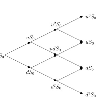
for i= 0,1, ..., n−1. We again assume we have an arbitrage-free market, i.e. d <1 +r∆t < u. S0 uS0 dS0 u2_S 0 udS0 d2_S 0 u3_S 0 uS0 dS0 d3S0

Figure 2.3: One-dimensional binomial tree with 3 steps

Assume we have a one-dimensional Black-Scholes model with stock price dynam-ics under the risk-neutral measure given by

dS(t) =S(t)(rdt+σdWt), S(0) =s0 >0,

whereσ >0 is volatility parameter, r is the risk-free interest rate andW is a one dimensional Brownian motion with respect to the risk-neutral measure Q. The time horizon T >0 is fixed.

The focus of this section is on risk-neutral binomial approximations to the log-normal stock price process. In the theory of option pricing a fundamental result states that in a complete market the option price is given as the discounted expected payoff under the risk-neutral measure Q

(27)

2.3. Binomial trees

EQ e−rTg(S(t), t∈[0, T])

, (2.3.2)

where g is a payoff function of the path-dependent financial instrument with maturity T and underlying S. Here we are interested mostly in European and American put and call options. We will consider American options in greater de-tail in Chapter 5. Usually, this expectation cannot be calculated explicitly so we have to apply numerical methods to approximate the desired quantity. The most famous numerical methods are Monte Carlo simulations, numerical methods for PDEs and the lattice approach. The topic of this thesis is the lattice approach, more precisely binomial trees.

What is a lattice approach? The aim of the lattice approach is to construct a discrete-time process S(n) _{and we want that this process converges weakly to our} continuous-time process S. On the next couple of pages we will explain how to do it.

Let us put now the binomial tree in a more formal shape. Ifn ∈_Nis the number of periods in the discrete model, then in binomial approximation of the stock price we have two possible scenarios per period

E(n) :={ω :{1,2, ..., n} → {1,−1}} endowed with the product σ-field

F(n)_:=

n

O

k=1

P({1,−1}) :=σZ_k(n)|k = 1,2, ..., n.

Here P(.) is a power set and Z_k(n) : E(n) _{→ {1,}_−1} _{is the coordinate mapping} with Z_k(n)(ω) = ωk.

Now we can define a binomial process on E(n)_,_F(n)

with the same starting point as the initial value of the continuous time process s0

S(n)(k+ 1) =S(n)(k)eα(n)∆t+β√∆tZ_k(n₊₁)_{, k} _{= 0,}_{1, ..., n}₋₁ _(2.3.3)

where β > 0 is a constant , α(n) is a deterministic function ofn and ∆t = T n is

the grid size of the discrete time model. From here we have that

u=u(n) :=eα(n)∆t+β √ ∆t and d=d(n) :=eα(n)∆t−β √ ∆t (2.3.4)

(28)

Theorem 2. (Risk-neutral valuation and replication)Each optiong in an n-period binomial model can be replicated by an investment strategy in the stock and the bond. The initial costs of this strategy determine the option price and are given by

c0 =EQ(n)(e−rTg),

where the measure Q(n) _{is the product measure of the one-period transition}

mea-sures Q(_in) which are determined by

Q(_in) S (n) i+1 S_i(n) = u ! =q= e r∆t₋_d u−d ,

and for which we have

S₀(n)=E_Q(n)(e−rTS_n(n)).

From the last equation, we can see that the expected relative return of the stock and the bond, under the measure Q(n), coincide. This motivates calling Q(n) the risk-neutral measure. The risk-neutral probability q gives us the market view on the likelihood that the favorable one-period returnuis attained and it can be dif-ferent from the physical probabilityp. More details can be found in, e.g [23], [25]. Let us now generalize this approach. For that purpose we will give two algorithms: one for European options and later one for American options.

The algorithm

Consider first a path-independent European option, i.e. an option with payoff g(ST), which can only be exercised at maturity. We want to approximate the

price EQ(g(S)) by using En(g(S(n))). The next algorithm explains how to do it:

1. Tree initialization

• Calculate the possible values of the stock at maturity S_k(n₊₁) =S_k(n)eα(n)∆t+β

√

∆tZ_k(n₊₁)_{, k} _{= 0,}_{1, ..., n}₋₁

• Calculate the option value at maturity V(n)(T, Sn(n)) =g(S

(n)

n )

for all possible values ofSn(n).

(29)

2.4. Trees and continuous-time models • Fori=n−1, ...,0 do V(n)(i∆t, S_i(n)) = e−r∆thqV(n)((i+ 1)∆t, uS_i(n)) + (1−q)V(n)_((i_{+ 1)∆t, dS}(n) i ) i 3. Return En(g(S (n)

n )) = Vn(0, s) as the discrete time approximation for the

option price,S₀(n) =s.

The option price is equal to its expected payoff in a risk-neutral world discounted at the risk-free interest rate. If we add more steps to the binomial tree, the risk-neutral valuation principle will still hold.

2.4 Trees and continuous-time models

As we have seen, a binomial approach leads to a modeling framework for option pricing which is easy to compute. Naturally, we are now interested if our model is in any reasonable way related to the Black-Scholes stock price model for which the stock price{St, t∈[0, T]}is assumed to follow a geometric Brownian motion,

i.e. St=s·exp r− 1 2σ 2 t+σWt ,

whereWt is one-dimensional Brownian motion andσ > 0 a given constant which

describes the volatility of the stock price movements. More precisely, as the period length ∆t tends to zero

• do we have weak convergence of the stock price paths in the sequence of increasing binomial models to the given geometric Brownian motion? • does the sequence of binomial option prices E_Q(n) e−rTg

n converge to

the corresponding option price in the Black-Scholes model?

The answer to these questions is related to the concept of weak convergence of the corresponding stochastic process. The Central Limit Theorem and Donsker’s theorem are here very helpful.

2.4.1 Weak convergence

(30)

Definition 3. Let M be a metric space with the Borel σ-field B(M), i.e. the smallest σ field containing all open subsets of M, and let Pn, n ∈ N, and P be

probability measures on(M,B(M)). The sequence{Pn}is said to converge weakly

to P, denoted by

Pn w

=⇒P,

if for every bounded, continuous function f :M →_R we have

lim n→∞ Z M f(x)dPn(x) = Z M f(x)dP(x).

Moreover, if Xn and X are random variables, n ∈N, with state space M defined

on probability space (Ωn,Fn, Pn) and (Ω,F, P) respectively, then the sequence

{Xn} is said to converge weakly to X, denoted by

Xn w

=⇒X,

if for every bounded, continuous function f :M →_R we have

lim

n→∞EPn(f(Xn)) =EP(f(X)),

i.e. if the corresponding probability distributions converge weakly.

Weak convergence of random variables is the same as weak convergence of their distributions. The range of all the random elements has to be the same, while the underlying probability spaces may be different.

One of the main results of weak convergence is Donsker’s Theorem which can be seen as a process version of the Central Limit Theorem. Here we will give a special case of it

Theorem 3. Donsker’s theorem (special case)For given stock price param-eters r (drift) and σ (volatility) the price process of the binomial tree converges (in distribution) towards the price process in the Black-Scholes model if the first two moments of the relative log-returns of both models coincide, i.e. if we have

E ln S(∆t) S(0) = E(n) ln S(n)₍₁₎ S(n)₍₀₎ E ln S(∆t) S(0) 2! = E(n) ln S(n)₍₁₎ S(n)₍₀₎ 2! .

By Donsker’s theorem, to achieve weak convergence, we need to have the first two moments of the log-increments of the discrete and the continuous model matched. For practical purposes, it is very important that weak convergence also holds if

(31)

2.4. Trees and continuous-time models

the moment matching conditions are only valid asymptotically (see [33]). To achieve that, we will choose the sequance (α(n))_n, the constant β > 0 and the sequence of probability measures P(n)

n on E

(n)_,_F(n)

n such that the following

conditions are satisfied:

1. ∀n ∈ _N, the random variables Z_k(n), k = 1,2, ..., n, are independent and identically distributed.

2. The first two moments of the one-period log-returns ofSare asymptotically matched, i.e. µ(n) : = 1 ∆tEP(n) ln S(n)_(k_{+ 1)} S(n)_(k) S(n)(k) = 1 ∆tEP(n) ln S(n)(k)eα(n)∆t+β √ ∆tZ_k(n₊₁) S(n)_(k) ! S(n)(k) ! =α(n) +β r 1 ∆tEP(n) Z_k(n₊₁) =α(n) +β r 1 ∆t(2pn−1) (2.4.1) σ2(n) : = 1 ∆tV arP(n) ln S(n)(k+ 1) S(n)_(k) S(n)(k) = 1 ∆tV arP(n) ln S(n)(k)eα(n)∆t+β √ ∆tZ_k(n₊₁) S(n)_(k) ! S(n)(k) ! = 1 ∆tV arP(n) α(n)∆t+β√∆tZ_k(n₊₁) =β2V ar_P(n) Z_k(n) = 4β2_p n(pn−1) (2.4.2)

are such that as n→ ∞,

µ(n)→r− 1 2σ

2 _(2.4.3)

and

σ2(n)→σ2. (2.4.4)

Under these conditions we will have that the linear interpolation of S(n)(k+ 1) =S(n)(k)eα(n)∆t+β

√

∆tZ_k(n₊₁)

, k = 0,1, ..., n−1

converges weakly to the stock price process. The drift parameteres (α(n))_n are allowed to be non-constant inn. The schemes withα(n)≡αconstant are referred to as conventional schemes. We will impose following condition:

(32)

Assumption:The sequence (α(n))_nis assumed to be bounded, i.e. it is assumed to be of order O(1).

The next theorem tells us the conditions which should be satisfied so that we have (2.4.3) and (2.4.4) (see [25] and [33], Proposition 2, page13).

Theorem 4. (Theorem on drift invariance) Let S(n) _{be a risk-neutral}

bi-nomial scheme. Then the moment matching conditions (2.4.3) and (2.4.4) are satisfied if and only if β =σ. In particular, convergence to the first two moments of the one-period log-returns in the continuous time model is of order

µ(n)− r− 1 2σ 2 =O 1 n and σ2(n)−σ2=O 1 n . (2.4.5)

Proof. By Taylor expansion of the exponential function and (2.3.4) we have u(n) = 1 +β T n 1₂ + α(n) + 1 2β 2 T n + 1 6β 3₊_α(n)β T n 3₂ + 1 2α 2_{(n) +} 1 2β 2_{α(n) +} 1 24β 4 T n 2 +o 1 n2 d(n) = 1−β T n 1₂ + α(n) + 1 2β 2 T n − 1 6β 3₊_α(n)β T n 3₂ + 1 2α 2_{(n) +} 1 2β 2_{α(n) +} 1 24β 4 T n 2 +o 1 n2 which implies q(n) = e r∆t₋_d(n) u(n)−d(n) = 1 2 +c1(n) T n 1₂ +c2(n) T n 3₂ +o 1 n32 (2.4.6) with c1(n) = 1 2β r−α(n)− 1 2β 2 c2(n) = 1 2β 1 2(α(n)−r) 2 + 1 6β 2_(α(n)₋_{r) +} 1 24β 4

where we used a Taylor expansion forer∆t, too. We should notice that c1(n) and c2(n) are of order O(1). Now consider

(33)

2.4. Trees and continuous-time models µ(n)(2.=4.1)α(n) +βn T 1₂ (2q(n)−1) =r− 1 2β 2 + 2βc2(n)T n +o 1 n and σ2(n)(2.= 4β4.2) 2_q(n)(1₋_{q(n)) =} _β2₋_4β2_c2 1(n) T n +o 1 n .

The moment matching conditions (2.4.2) and (2.4.3) are satisfied if and only if β =σ. From those equations we can also conclude that

µ(n)− r− 1 2σ 2 =O 1 n and σ2(n)−σ2=O 1 n

which proves the theorem.

We have only a condition onβ, i.e. the weak convergence is ensured independently of the choice of the sequence (α(n))n. This leaves space for suitable good choices

of α(n) to improve the convergence behavior. These choices will play a central role in the next chapter where we will concentrate more on the choice of the drift parameter and explore more properties of it.

2.4.2 CRR and RB trees

In Theorem 4 we have seen some conditions which a binomial tree should satisfy such that we have week convergence to the Black-Scholes stock price process. This means, if we have a bounded payoff, the parameters of the binomial tree must be chosen such that option prices converge to the continuous-time limit, i.e. discrete distribution of the asset price (represented by the binomial tree) must converge to the continuous-time limit of the lognormal distribution. As we have shown in the previous section, this means that we must have (approximate) equality of the first two moments of continuous and discrete model. There are many possibilities to satisfy the moment matching conditions since we have two equations and three parameters: p,u and d. In this chapter we will focus on two of them. The first suggestion was given by Cox, Ross and Rubinsten (CRR from now on) in [9] and they suggested the following parameters:

u=eσ √ ∆t_{, d}₌ 1 u, p= 1 2 1 + r− 1 2σ 2 1 σ √ ∆t . Since p is a probability of an up-movement, it is only well defined if

0≤ 1 2 1 + r− 1 2σ 2 1 σ √ ∆t ≤1 ⇐⇒ n > (r− 1 2σ 2₎2 σ2 T.

(34)

Here we have α ≡ 0 and β = σ. For these parameters we have that the first moment of the log increments is exactly matched but the second one is matched asymptotically: µ(n) = r− 1 2σ 2_, σ(n)2 ₌_σ2₋ r− 1 2σ 2 2 ∆t.

Another property of this model is, since α ≡ 0, there is no drift and the tree is symmetric in the log-scale around the initial value log(S0).

The main drawback of this model is that the convergence is not smooth. We will later show that the order of convergence isO√1

n

, but since it is not smooth we cannot apply an extrapolation method to speed it up. Also oscillations between even and odd n can be observed. This is known as the even-odd effect. But if we consider only even n(or odd n) then these oscillations are not present. In the Figure 2.4 the even-odd problem is shown. More details about the convergence of the CRR tree are presented in Section 3.1.

200 400 600 800 1000 11.65 11.66 11.67 steps option price CRR BS

Figure 2.4: European call option price obtained using CRR model: S0 = 95, K = 100, σ = 0.25, r = 0.1,T = 1, Black-Scholes = 11.6573.

The second suggestion was given by Rendleman and Bartter [40](RB from now on): p= 1 2, u=e (r−1 2σ 2_)∆_t₊_σ√_∆_t , d=e(r−12σ 2_)∆_t₋_σ√_∆_t ,

(35)

2.4. Trees and continuous-time models

and with these parameters we match both moments exactly. Here we haveα=r− 1

2σ

2_{, which means this tree is tilted with regard to initial value, but the probability} p is fixed which is an advantage in the implementation of the model since it requires less operation counts because of the symmetry in the probabilities. This speeds up the algorithm. The RB model unfortunately also suffers from irregular convergence which can be seen in Figure 2.5.

200 400 600 800 1000 11.65 11.66 11.67 steps option price RB BS

Figure 2.5: European call option price obtained using RB model: S0 = 95, K = 100, σ = 0.25, r = 0.1,T = 1, Black-Scholes = 11.6573.

A comparison between these two models is given in Bock [1], where the author has shown that the absolute error for both models has a very similar convergence pattern, but the CRR model delivers better results for the relative error. In this thesis the focus will be on the models derived from the CRR model.

(36)

(37)

25

Chapter 3 Advanced and modified trees

In the previous chapter we have seen the basic structure of the binomial trees. Now the natural question which arises is: can we have better results using suitably modified binomial trees? Answering this question will be the main topic of this chapter.

3.1 Why and when is a CRR tree good?

Let us first look in great detail at the convergence behavior of the CRR tree. Diener and Diener showed in [10] that the convergence rate for CRR trees for European calls is O _n1. We want to see now under which circumstances we get the best behavior of the CRR tree. These results will motivate us to introduce modified binomial trees. We will first focus on results given by Diener and Diener and afterwards we will expand our research. Their result in our notation is: Theorem 5. In the n-period CRR binomial model, if S0 = 1, the binomial price

C(n) at t = 0 of the European call with strike price K and maturity T = 1

satisfies C(n) =CBS+ e−d 2 1 2 24σ√2π A−12σ2_(∆2 n−1) n +O( 1 n√n), where ∆n= 1−2 ( ln(S0 K) +nlnd ln(u d) ) , A=−σ2_{(6 +}_d2 1+d 2 2) + 4(d 2 1−d 2 2)r−12r 2_,

{x} is the fractional part of x, CBS is the price obtained by the Black - Scholes

formula and d1 and d2 are the coefficients in the Black - Scholes formula, i.e. as

(38)

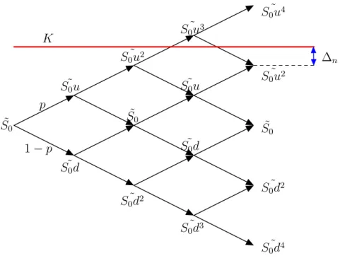
p 1−p ˜ S0 ˜ S0u ˜ S0d ˜ S0 ˜ S0 ˜ S0u2 ˜ S0d2 ˜ S0u3 ˜ S0u ˜ S0d ˜ S0d3 ˜ S0d4 ˜ S0d2 ˜ S0u2 ˜ S0u4 K ∆n

Figure 3.1: Binomial tree with ∆n, log-scale

As we can see, the coefficient of 1

n in the error depends on the quantity ∆n. Let

us investigate this coefficient.

Let l:=l(n) be an integer value such that

S(n)(l−1) :=S0ul−1(n)dn−l+1(n)< K ≤S0ul(n)dn−l(n) :=S(n)(l),

i.e. S(n)(l−1) and S(n)(l) are the terminal nodes adjacent to the strike value K. The non constant factor ∆n can be rewritten also for the general type of trees,

i.e. using u(n) andd(n) from (2.3.4) we get (with, of course β =σ)

∆n:= 1−2{−a(n)}:= 1−2 ( −1 2n+ ln s0 K +α(n)T 2σ√T √ n ) . (3.1.1) Chang and Palmer have shown in [7] that ∆n can also be represented as

∆n= 1−2

lnS(n_K)(l) ln_SS(n()n₍)_l(₋l)₁₎

. (3.1.2)

and thus, it measures the distance between the strike value and its adjacent ter-minal values in log-scale, which is illustrated in Figure 3.1. Now we can conclude

(39)

3.1. Why and when is a CRR tree good?

that ∆n is strictly increasing on S(n)(l−1), S(n)(l)

with ∆n = ( 1 forK =S(n)(l) 0 forK =pS(n)_(l₋_1)S(n)_(l) , (3.1.3) and it converges to −1 as K tends to S(n)_(l ₋_{1). This is the reason why we} have oscillations in the CRR binomial call price around the Black - Scholes price. Controlling this might help us getting smooth convergence.

Let a(n) be, as in (3.1.3), the quantity

a(n) := ln K S0 −nlnd lnu−lnd . (3.1.4) Then we have

[x] := k(n) := [a(n)] + 1 =a(n) + 1− {a(n)}, (3.1.5) where [x] denotes the integer part of x and {x} :=x−[x]. Then, the fractional part {a(n)}is always bounded between 0 and 1.

Now we assume the following: u and d have a converging expansion of type u=u(n) = 1 2+σ 1 √ n +u2 1 n +... d=d(n) = 1 2 −σ 1 √ n +d2 1 n +...

For example, parameters u and d from the CRR model satisfy this converging expansion. Then we have the following result (see [10])

Corollary 3. The integer k(n) defined by (3.1.5) has the following asymptotic expansion with bounded coefficients:

k(n) = 1 2n+a−1 √ n+a0+ 1− {a(n)}+O 1 √ n (3.1.6) where a−1 = 1 4σ 2 ln K S0 −(u2+d2) +σ2 , a0 = 2 2 ln K S0 −(u2+d2)−σ2 (u2−d2))

(40)

This means, the function a(n) has an asymptotic expansion of typea(n) = 1 2n+ a−1 √ n+O√1 n

in the model under consideration here. The first term does not give any contribution to k for even n (its fractional part is zero), and for odd n it brings a contribution of 1

2 to k. This explains the oscillations of order 1

n

between even and odd values ofn in the priceC(n). Further, for the same parity of n, when a(n) is far away from an integer value, its fractional part k changes continuously, but it will have a discontinuity every time a(n) crosses an integer. On the other hand, in the case of the call at the money, i.e. K = S0, one has a(n) = n

2 (for the CRR tree, i.e. when u= 1

d) and thus the price C(n) oscillates

but the asymptotic expansion with bounded coefficient is much easier to compute as k is simply equal to 0 for even n and 1

2 for odd n. Thus, there is no scallop here. In Figure 3.2 we can see that the CRR tree is indeed smooth for K =S0. We will take this up again in a more general setting when introducing the split tree in Chapter 4. 200 400 600 800 1000 5.435 5.445 5.455 5.465 steps option price CRR BS

Figure 3.2: European put option obtained using CRR model: S0 = 100,K = 100, σ = 0.25, r = 0.1, T = 1, Black-Scholes =5.4595

Now combining all these results we end up with

Corollary 4. The CRR tree admits a smooth convergence for S0 = K and the

order of it for this case is O _n1.

We have seen that the CRR model behaves better compared to other models in case of S0 =K, i.e. there is no scallop. But, usually we have initial values given

(41)

3.2. Advanced trees

and we cannot choose them freely. Can we maybe create a similar behavior of the CRR tree if we plays it suitably around K? Answering this question will be the main idea of the next few sections.

From now on, we will say that u=eασ2∆t+σ √ ∆t , d=eασ2∆t−σ √ ∆t

where α = α(n) is in general a bounded sequence depending of n. In [7] they consider all possible choices of u and d such that u

d = e

2σ√∆t _and _n_{ln(ud) is}

bounded. If we look at our statement again, we will see that these two statements are equivalent. This is a more general approach, since forα = 0 we get the CRR model, for α = r

σ2 −

1

2 we get the RB model. The reason why we consider this more general case is that it allows us to see how our tree behaves for different values of α, also known as a drift.

3.2 Advanced trees

In [7] Chang and Palmer concentrated on getting smooth convergence rather than faster convergence, since once we have smooth convergence we can apply extrapolation methods and improve our rate of convergence. The next theorem is the main theorem from [7] and it tells us that the rate of convergence of digital and European options is O _n1 but it gives us motivation how to improve the results. It is a slight generalization of Diener and Diener [10], but it has a simpler proof.

Theorem 6 (Main Theorem - Chang and Palmer). For the n-period binomial model, where

u=eασ2∆t+σ

√

∆t_{, d}₌_eασ2_∆_t₋_σ√_∆_t

, (3.2.1)

with α an arbitrary bounded function of n, if the initial stock price is S0 and the

strike price is K with maturity time T. Then 1. the price of a digital call option satisfies

Cd(n) =e−rTΦ(d2) + e −rT_e −d2₂ 2 √ 2π h ∆n √ n − d2∆2 n 2n + Bn n i +O 1_n and

(42)

C(n) =CBS+ S0e −d 2 1 2 24σ√2πT An−12σ2T(∆2n−1) n +O( 1 n), where Bn = d3 1+d1d22+2d2−4d1 24 + (2−d1d2−d2 1) √ T 6σ (r−ασ 2_{) +} T d1 2σ2(r−ασ2)2, An =−σ2T(6 +d12+d22) + 4T(d21−d22)(r−ασ2)−12T2(r−ασ2)2.

The price of a European call option with maturity T is given by (from [37]): C(n) = S0 n X k=j n k ˆ pkqˆn−k−Ke−rT n X k=j n k pkqn−k, where 0< p <1,p= er∆t−d u−d , q= 1−p, ˆp=pue −r∆t_{, ˆ}_q_{= 1}₋_p_ˆ_and j = [γ] whereγ = lnK S0 −nlnd ln u d .

The price of a digital call option is given by:

Cd(n) = e−rT n X k=j n k pkqn−k

and its Black-Scholes price is given by e−rT_Φ(d_{2), while for the European call it}

is given by SΦ(d1)−Ke−rT_Φ(d_2).

The following lemma, an extension of a result of Uspensky from [48], is our fundamental tool for proving the Main theorem, Theorem 6.

Lemma 1. Provided that p → 1

2 as n → ∞ and 0 ≤ j = jn ≤ n + 1 for n sufficiently large, n X k=j n k pkqn−k = √1 2π ξ2 Z ξ1 e−u 2 2 du+ q−p 6√2πnpq (1−ξ₂2)e−ξ 2 2 2 −(1−ξ2 1)e −ξ 2 1 2 + 1 12n√2π ξ2e− ξ2₂ 2 (ξ2 2 −1)−ξ1e− ξ₁2 2 (ξ2 1 −1) +o 1 n , where ξ1 = j−np−1 2 √ npq and ξ2 = nq+1₂ √ npq.

(43)

3.2. Advanced trees

Proof of the Main theorem. Assume that n is large enough such that we have 0< p <1 and 0≤γ ≤n+ 1, which implies that 0≤[γ]≤n+ 1.

Proof of part 1: Let us first expand probability p in powers of ∆t12 up to third

order. Then by definition of u and d and using the Taylor expansion

p= e r∆t₋_d u−d = 1 2 +α∆t 1 2 +β∆t 3 2 +o ∆t32 (3.2.2) where α= r−(λ+ 1 2)σ 2 2σ , β= σ4_(4λ_{+ 1)}₋_4σ2_r_{+ 12(r}₋_λσ2₎2 48σ . Next, we compute ξ1 = j−np− 1 2 √ npq =− 1 2√npq(−2j+ 2np+ 1). (3.2.3) Since j =γ+{−γ},−2γ+n+ 2nα∆t12 =d₂ √ n and using (3.2.2): −2j+ 2np+ 1 =−2j+ 1 +n+ 2nα∆t12 + 2nβ∆ 3 2 +o(∆t 1 2) = ∆n+d2 √ n+ 2βT∆t12 +o(∆t 1 2). (3.2.4) Also, because pq=p(1−p) = 1 4 −α

2_∆t3₂ _{and using the binomial series theorem} 1

2√pq = 1 + 2α

2_∆t₊_O(∆t3₂_). _(3.2.5) Hence, using (3.2.3), (3.2.4) and (3.2.5)

−ξ1 =d2+ ∆n √ n + δ n +o 1 n ,with δ= 2T(α2_d 2+β √ T). (3.2.6) Next, we examine the terms in Lemma 1 one by one. Let

I := ξ2 Z ξ1 e−u 2 2 du= ∞ Z ξ1 e−u 2 2 du− ∞ Z ξ2 e−u 2 2 du=:I1−I2.

(44)

First we estimate I1. Using f(x) := x R d2 e−u 2

2 du, which is an even function, we get

I1 = −ξ1 Z −∞ e−u 2 2 du = d2 Z −∞ e−u 2 2 du+ −ξ1 Z d2 e−u 2 2 du= Φ(d2) √ 2π+f(−ξ1). For some η between −ξ1 and d2, by a Taylor expansion we have

f(−ξ1) =e− d2₂ 2 (−ξ 1−d2)− d2e− d2₂ 2 2 (−ξ1−d2) 2₊f 000 (η) 3! (−ξ1−d2) 3_,

where f000(η) =−e−η₂2 ₊_η2_e−η₂2 _{is bounded. Then it follows from (3.2.6) that}

f(−ξ1) =e−d 2 2 2 ∆n √ n + δ n − d2∆2n 2n +o 1 n , so I1 = Φ(d2) √ 2π+e−d 2 2 2 ∆n √ n + δ n − d2∆2 n 2n +o 1 n . (3.2.7) Now we are going to estimate I2. Since p → 1

2 and q → 1 2 as n → ∞, we have ξ2 √ n = nq+1₂

n√pq → 1 as n → ∞, which implies that we can find n0 such that ξ2 ≥ 2

for n≥n0. Then, when n ≥n0,

|I2| ≤ ∞ Z ξ2 e−udu=e−ξ2 =e− nq+ 1₂ √ npq ₌_o 1 n . (3.2.8) From (3.2.5) and (3.2.2) 1 2√pq = 1 + 2α2_T n +O 1 n32 p−q= 2α √ T √ n +O 1 n32 so that we have q−p √ npq =− 4α√T n +O 1 n2 .

(45)

3.2. Advanced trees

Next, note that (1−ξ2 2)e −ξ22 2 −(1−ξ2 1)e −ξ21 2 → −(1−d2 2)e −d22 2 as n→ ∞. Hence q−p 6√2πnpq (1−ξ₂2)e−ξ 2 2 2 −(1−ξ2 1)e −ξ21 2 = −4α √ T 6n√2π −(1−d2₂)e−d 2 2 2 +o 1 n . (3.2.9) Using −ξ1 →d2 and ξ2 → ∞ asn → ∞, we get

1 12n√2π(ξ2e −ξ 2 2 2 (ξ2 2 −1)−ξ1e− ξ2₁ 2 (ξ2 1 −1)) = d2e− d2₂ 2 (d2 2−1) 12√2π 1 n +o 1 n . (3.2.10) Putting (3.2.7) - (3.2.10) in Lemma 1, we obtain

erTCd(n) = n X k=j n k pkqn−k = Φ(d2) + e −d 2 2 2 √ 2π ∆n √ n − d2∆2 n 2n + " δ+ 2α √ T 3 − d2 12 ! (1−d2₂) # 1 n ) +o 1 n . (3.2.11)

Now multiplying the last term bye−rT _{and replacing}_α_and _δ_{by their definitions,}

we prove the first part of the main theorem.

Proof of part 2: Now we will use Lemma 1 with p, q,ξ1, ξ2 replaced by their hatted versions ˆp, ˆq, ˆξ1, ˆξ2 and obtain

n X k=j n k ˆ pkqˆn−k = √1 2π ˆ ξ2 Z ˆ ξ1 e−u 2 2 du+ qˆ−pˆ 6√2πnˆpˆq (1−ξˆ₂2)e− ˆ ξ2₂ 2 −(1−ξˆ2 1)e −ξˆ 2 1 2 + 1 12n√2π ˆ ξ2e− ˆ ξ2₂ 2 ( ˆξ2 2 −1)−ξ1eˆ −ξˆ 2 1 2 ( ˆξ2 1 −1) +o 1 n , where ˆ ξ1 = j−npˆ− 1 2 √ npˆˆq and ˆξ2 = nqˆ + 12 √ npˆˆq.

(46)

Our next step is to estimate ˆp. Using formula (3.2.1) and another Taylor expan-sion, we arrive at ˆ p= u−ude −r∆t √ npˆˆq = 1 2 + ˆα∆t 1 2 + ˆβ∆t 3 2 +o ∆t32 where ˆ α= r−(λ− 1 2)σ 2 2σ , β = σ4_(4λ₋₁₎₋_4σ2_r₋_12(r₋_λσ2₎2 48σ . (3.2.12)

Now by replacingp,q,αandβ in the derivation of (3.2.6) by the same quantities with hats on and using the fact that −2γ+n+ 2nα∆tˆ 12 =d₁

√ n, we get −ξˆ=d1+ ∆n √ n + ˆ δ n +o 1 n , where ˆδ= 2T(ˆα2d1+ ˆβ √ T).

Proceeding as we did to get (3.2.11) and using the hatted version of p, q, ξ1, ξ2, α, β, δ and using d1 instead of d2, we obtain the relation

n X k=j n k ˆ pkqˆn−k = Φ(d1) + e −d1 2 √ 2π × ( ∆n √ n + " ˆ δ− d1∆ 2 n 2 + 2ˆα√T 3 − d1 12 ! (1−d2₁) # 1 n ) +o 1 n . (3.2.13) Now if we multiply (3.2.13) with S0, (3.2.11) with Ke−rT_{, then subtracting and}

using S0e− d2₁ 2 =Ke−rTe− d2₂ 2 , we get C(n) = S0Φ(d1)−Ke−rTΦ(d2) + S0e− d2₂ 2 C_n √ 2π 1 n +o 1 n , where Cn is Cn= ˆδ−δ− σ∆2 n √ T 2 + (1−d2 1) √ T 12 (8−(ˆα−α)−σ)− σ√T(d1+d2) 12 (8α−d2). Simplifying the last equation we get the second part of the Main theorem.

In the Main theorem we have again the coefficient ∆n. Until now we just proved

the theorem, but our next step is to use it and see how we can improve our results by controlling this coefficient.

(47)

3.2. Advanced trees

3.2.1 The Tian tree

Convergence in the CRR and RB trees is almost always nonsmooth because the position ofK oscilates between the two adjacent stock prices so that ∆noscillates

between 1 and -1. To overcome this problem, Tian [47] suggested that we take a new drift which will move our tree such that the adjacent node is placed exactly at the pointK, i.e. ∆n = 1. This will be done in the following way: We determine

the node closest to the strike price K by solving the following equation: K =S0u(n)ad(n)n−a.

This leads us to:

a(n) = lnK S0 −nln (d(n)) ln(u(n))−ln(d(n)) .

The right hand side of the last equation is usually not an integer, i.e. lα(n)−1<

a(n)< lα(n), lα(n) ∈ N. To ensure that the terminal node is placed exactly on

the strike value K, for the given sequence (lα(n))n we define sequence (˜α(n))n

such that ˜ α(n) := lnK S0 −(2lα(n)−n)σ √ ∆t T . (3.2.14)

For any number of periodsn, the Tian modelS_α(_˜n₍_n)₎is defined as the process (2.4.1) with β = σ and with the new drift ˜α(n). The new parameter is not constant, it depends on the number of periods. The process S(n)

e

α(n) is defined such that the corresponding equation K =S0u(n)ad(n)n−a is solved by

a e α(n)(n) = 1 2n+ lnK S0 −α(n)T_e 2σ√T √ n =lα(n), (3.2.15)

where the last equation follows from (3.2.14). It follows now that the quantity aα(n) obtained for the Tian model is integer-valued. Hence,

ln S(n) e α(n)(l) K ln S(n) e α(n)(l) S(n) e α(n)(l−1) = 0 i.e. by (3.1.3) S(n) e α(n) =K,∀n ∈N.

(48)

This means that for any number of periods n, the terminal distribution of the Tian model assigns probability mass to the point K. As a consequence, we get ∆n= 1, i.e. it does not depend on n.

It is left to show that the model suggested by Tian converges to the Black -Scholes value, i.e. we have to ensure weak convergence. Since we have β =σ, it is left to show that the sequence of drift parameters (α(n))_e n) is bounded. In that

case, the moment matching conditions are satisfied for the risk-neutral transition probabilities and weak convergence follows by the Main theorem. Comparing to the CRR model, in Tian’s model the mass points are moved by a small distance. This can be seen by writing the new drift (α(n))e n) in terms of the original one. By (3.2.14) and (3.2.15):

e

α(n) = √2σ

T√n(aα(n)−lα(n)) +α, and this implies, since −1≤aα(n)−lα(n)≤0,

−√2σ

T√n +α ≤α(n)e < α.

Observe that the new drift α(n) in Tian’s model differs from the original drift bye e

α(n) = α+o(1). (3.2.16) Moreover, the new drift satisfies Assumption 1, i.e. α(n) =_e O(1), and we can formulate:

Proposition 1. The sequence of processes S(n) e

α(n)

n∈_N defined by Tian’s model

with linear interpolation and an appropriate time-scaling converges weakly to the stock price process S.

Since ∆n is found to be independent of n, compared to other methods with

constant drift α, Tian’s model shows a more improved convergence behavior of the discretization error in the approximation of the terminal stock price. Let us now see how the Main theorem changes with ∆n obtained by Tian’s model.

Proposition 2. LetK ∈_R. The binomial modelS_{T ian}(n) suggested by Tian admits the following representation of the discretization error:

• The discretization error of the digital call option is

Cd(n) = e−rTΦ(d2) + e−rT_e−d 2 2 2 √ 2π 1 √ n − d2 2n + Bn n +O 1 n and

(49)

3.2. Advanced trees

• The discretization error of the price of a European call options satisfies

C(n) =CBS+ S0e− d2₁ 2 24σ√2πT An n +O 1 n , where Bn = d3 1+d1d22+2d2−4d1 24 + (2−d1d2−d2 1) √ T 6σ (r−ασ 2_{) +} T d1 2σ2(r−ασ2)2, An =−σ2T(6 +d12+d22) + 4T(d21−d22)(r−ασ2)−12T2(r−ασ2)2.

In Tian’s model, the discretization error converges smoothly along the upper bound given by exp−12d

2 2(x)

√

2πn

. The convergence for digital options is not faster, but for European call options we get convergence order O _n1. By smooth con-vergence we imply that the coefficient of the leading error term is constant and the oscillations of the higher order terms are negligible. As a result, the Berry Ess´een bound remains tight and extrapolation methods can be applied.

As we already know, the CRR model is not smooth, but we have just shown that Tian’s model is. The model suggested by Tian shows smaller pricing errors as more time steps are used, which is not the case in the CRR model. The rate of convergence is not improved, but this is not a drawback since extrapolation methods can be used to improve the rate of convergence.

We applied Tian’s model to the same example as we did with the CRR and RB models, where irregular convergence and the even-odd problem was visible. In Figure 3.3 the even-odd problem is still noticeable, but the scallop effect is gone. To avoid the even-odd problem, in practice we usually use only even or odd step numbers. If we now look at Figure 3.4, we can notice the almost smooth convergence and that the even-odd oscillations have disappeared.

3.2.2 The Chang and Palmer tree

Similar to Tian’s approach, Chang and Palmer [7] (CP from now on) suggested that we move our tree such that the strike value is placed on the geometric average of two adjacent nodes, i.e. to have ∆n = 0. The original drift α in this

model is replaced by some sequence of drift parameters (α(n))_n_∈

Nsuch that K = p

S(n)_(l(n))S(n)_(l(n)₋_{1). As a consequence, the discretization error will exhibit} a higher order of convergence. This model is also known as ”the centered binomial model”. Let us investigate this in more detail: Assume Sα(n) is the binomial

(50)

200 400 600 800 1000 11.62 11.63 11.64 11.65 11.66 steps option price Tian BS

Figure 3.3: European call option price obtained using Tian model: S0 = 95, K = 100, σ = 0.25, r = 0.1,T = 1, Black-Scholes =11.6573.

process (2.4.1) withβ =σandα(n) =α constant inn. As in Tian’s model,lα(n)

denotes the corresponding integers such that K ∈ Sn(n)(lα(n)−1), S

(n)

n (lα(n))

i . Then, the sequence for the new drift parameter will be given by

α(n) = lnK S0 −(2lα(n)−n−1)σ √ δt T . (3.2.17)

By (3.2.17) the CP model is defined such that the equations0u(n)ad(n)n−a =K is solved by aα(n)(n) := 1 2n+ lnK S0 −α(n)T 2σ√T √ n=lα(n)− 1 2. which leads us to ln S_α(n₍)_n₎(l) K ln S_α(n₍)_n₎(l) S_α(n₍)_n₎(l−1) = 1 2 i.e. by (3.1.3)

(51)

3.2. Advanced trees 200 400 600 800 1000 11.62 11.63 11.64 11.65 11.66 steps option price Tian BS

(a) Tian with even number of steps

200 400 600 800 1000 11.62 11.63 11.64 11.65 11.66 steps option price Tian BS

(b) Tian with odd number of steps

Figure 3.4: European call option price obtained using Tian model: S0 = 95, K = 100, σ = 0.25, r = 0.1,T = 1, Black-Scholes =11.6573.

(52)

K = q

S_α(n₍)_n₎(lα(n)−1)S

(n)

α(n)(lα(n)),∀n∈N. (3.2.18) As we can see from (3.2.18), for any number of periodsn, the terminal distribution of the corresponding CP model is such that the pointKis at the geometric average of two neighboring mass points. Now we can conclude, using (3.1.3), that in this model ∆n= 0 always and this will improve our order of convergence.

Our next aimis to show that we want to show α(n) = α + o(1). Since the probability mass is moved only by a small distance, this is a direct consequence. Similar to the case in Tian’s model, we can conclude

α(n) = √2σ T√n aα(n)−lα(n) + 1 2 +α, (3.2.19) whereaα(n) is solution of the equationS0u(n)ad(n)n−a =Kin the original model. From (3.2.19) α− √ σ T√n ≤α(n)< α+ σ √ T√n, which shows our assertion.

We now can conclude these results in the following position. Proposition 3. The sequence of processes

S_α(n₍_n)₎

n∈N

defined by the Chang and Palmer model with linear interpolation and an appropriate time-scaling converges weakly to the stock price process S.

Then, we can formulate the Main theorem as follows.

Theorem 7 (Main Theorem - Chang and Palmer). For the n-period binomial model, where

u=eασ2∆t+σ

√

∆t_, _d₌_eασ2_∆_t₋_σ√_∆_t

,

with α an arbitrary bounded function of n, if the initial stock price is S0 and the

strike price is K with maturity time T, we have that 1. the price of a digital call option satisfies

Cd(n) = e−rTΦ(d2) + e −rT_e−d 2 2 2 √ 2π Bn n +O 1 n and

(53)

3.2. Advanced trees C(n) =CBS+ S0e −d 2 1 2 24σ√2πT An+12σ2T n +O( 1 n), where Bn = d3 1+d1d22+2d2−4d1 24 + (2−d1d2−d2 1) √ T 6σ (r−ασ 2_{) +} T d1 2σ2(r−ασ2)2, An =−σ2T(6 +d12+d22) + 4T(d21−d22)(r−ασ2)−12T2(r−ασ2)2. This theorem tells us that the order of convergence is improved from _√1

n to

1

n for

both digital and European call options, i.e. we have lim sup n→∞ sup K∈R Q (n)_S(n) CP ≥K −Φ(d2(K)) √ n = 0 and lim sup n→∞ sup K∈_R Q (n)_S(n) CP ≥K −Φ(d2(K)) n >0,

which means if the binomial process is defined according to the CP model, the Berry-Ess´een bound ceases to be tight and, in addition, the leading discretization error term converges monotonically.

200 400 600 800 1000 11.66 11.675 11.67 steps option price CP BS

Figure 3.5: European call option prices obtained using CP model: S0 = 95, K = 100, σ = 0.25, r = 0.1,T = 1, Black-Scholes =11.6573.

(54)

200 400 600 800 1000 11.66 11.67 steps option price CP BS

(a) CP with even number of steps

200 400 600 800 1000 11.66 11.67 steps option price CP BS

(b) CP with odd number of steps

Figure 3.6: European call option prices obtained using CP model: S0 = 95, K = 100, σ = 0.25, r = 0.1,T = 1, Black-Scholes =11.6573.