Generation of Fuzzy Rules Based on Complex-valued Neuro-Fuzzy Learning Algorithm

(1)

Abstract. In order to generate or tune fuzzy rules, Neuro-Fuzzy learning algorithms with Gaussian type membership functions based on gradient-descent method are well known. In this paper, we propose a

new learning approach, the Complex-valued

Neuro-Fuzzy learning algorithm. This method is an extension of the conventional method to complex domain by using a complex-valued neural network that maps complex values to real values. Input, ante-cedent membership functions and consequent single-ton are complex, and output is real. Two-dimensional input can be better represented by complex numbers than by real values. We compared it with the con-ventional method by several function identification problems, and revealed that the proposed method outperformed the counterpart, and that it is a useful tool for learning a fuzzy system model.

Keywords: Neuro-fuzzy, Complex-valued neural networks, Fuzzy, Neural networks

1. INTRODUCTION

In the field of fuzzy control, the practical applications of fuzzy inference have increased, and generations of fuzzy rules have become important. These include tuning of membership functions and rules. However, when a fuzzy system model is designed, it is sometimes too hard or impossible for human beings to give the desired fuzzy rules, due to the ambiguity, uncertainty or complexity of the identifying system. Many methods have been con-structed by combining fuzzy systems and neural net-works to generate or tune fuzzy rules of fuzzy system models [1-6]. These methods, called Neuro-Fuzzy learning algorithms (NFs), recently have been success-fully applied to, e.g. control system and system identifi-cation [7 - 12]. Further, a variety of system structures and learning algorithms are available for NFs [13 - 15]. In this paper, we use a method of tuning fuzzy rules and its parameters by back propagation learning algorithm [16] of neural networks [1, 2]. Such NFs, whose ante-cedent membership function is fixed for each fuzzy in-ference rule under the simplified fuzzy inin-ference method, can generate fuzzy rules by automatic tuning of its pa-rameters and the consequent singleton values based on a gradient-descent method. However, if we use multi input for this method, a number of parameter of antecedent

membership function increase rapidly with increasing a number of fuzzy inference rules. For this reason, it takes a long period of time for learning and the learning accu-racy may deteriorate [3].

As a solution of these problems (the learning time and the learning accuracy), we focused on Complex Back Propagation (CBP) [17 - 19] of Complex-valued Neural Networks (CVNNs). CVNN is shown to be powerful in applications such as adaptive radar image processing, and optical image processing [20]. Further extension to multidimensional values has been attempted as well [21]. In addition, in our previous studies, we applied CVNN on real-valued classification problems and showed an efficient and good conversion [22, 23].

In this paper, we propose the Complex-valued Neuro-Fuzzy learning algorithm (CVNF). It extends the antecedent membership function and the consequent singleton of the conventional method to complex do-main and generates real-valued output for com-plex-valued inputs. Further, we compared it with the conventional method by several function identification problems, and show the superiority.

2. NF AND CVNF

2.1. Conventional NF

In the conventional NF, if the inputs are Xi (i = 1, 2, …,

n) and the output is Y, then fuzzy inference rules of the simplified fuzzy inference are shown below:

Rule 1: If X1 is M11 and X2 is M12 … Xn is M1n Then Y is W1 Rule 2: If X1 is M21 and X2 is M22 … Xn is M2n Then Y is W2 … Rule m: If X1 is Mm1 and X2 is Mm2 … Xn is Mmn Then Y is Wm (1) where Wj (j=1, 2, …, m) are real value of the consequent singleton.

Ryusuke Hata

1

, Md. Monirul Islam

2

, Kazuyuki Murase

1 1

Graduate School of Engineering, University of Fukui, Fukui, Japan

2_{Department of Computer Science and Engineering, Bangladesh University}

of Engineering and Technology, Dhaka, Bangladesh

Generation of Fuzzy Rules Based on Complex-valued

Neuro-Fuzzy Learning Algorithm

(2)

The antecedent membership functions Mji (j = 1, 2, …,

m; i = 1, 2, …, n) are given by Gaussian function as,

(2)

The inference result Y is as follows. First, the grade of the antecedent is given by

(j=1, 2, …, m) (3)

Then, the inference result Y is calculated by the follow-ing gravity method.

(4)

The error function to be minimized during the training is given by

(5) where T is the desired output. During the training, each parameter is updated by,

(6) (7) (8)

where are the learning rate.

We can perform the learning process by giving the ini-tial value to each parameter and by using equations Eq. (6) – (8).

2.2. The CBP

Before describing the CVNF, we should mention the CBP.

The CBP extends back propagation (RBP) to complex domain for learning a complex pattern. Previous study [17] showed properties of CBP as follows:

1) The CBP has a structure based on two dimensional motions.

2) The CBP promote the learning process as one unit complex signal through the network.

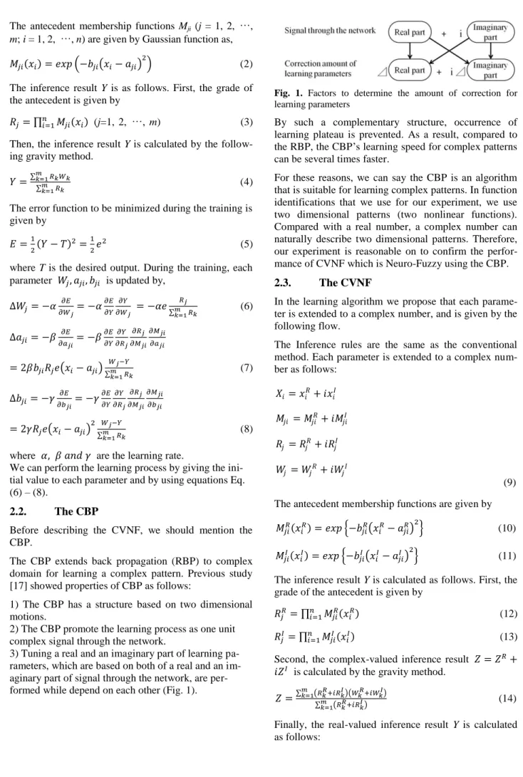
3) Tuning a real and an imaginary part of learning pa-rameters, which are based on both of a real and an im-aginary part of signal through the network, are per-formed while depend on each other (Fig. 1).

Fig. 1. Factors to determine the amount of correction for learning parameters

By such a complementary structure, occurrence of learning plateau is prevented. As a result, compared to the RBP, the CBP’s learning speed for complex patterns can be several times faster.

For these reasons, we can say the CBP is an algorithm that is suitable for learning complex patterns. In function identifications that we use for our experiment, we use two dimensional patterns (two nonlinear functions). Compared with a real number, a complex number can naturally describe two dimensional patterns. Therefore, our experiment is reasonable on to confirm the perfor-mance of CVNF which is Neuro-Fuzzy using the CBP.

2.3. The CVNF

In the learning algorithm we propose that each parame-ter is extended to a complex number, and is given by the following flow.

The Inference rules are the same as the conventional method. Each parameter is extended to a complex num-ber as follows: 𝑋_𝑖= _𝑖 + 𝑖 _𝑖𝐼 𝑗𝑖 = 𝑗𝑖 + 𝑖 𝑗𝑖𝐼 𝑗 = 𝑗 + 𝑖 𝑗𝐼 𝑗 = 𝑗 + 𝑖 𝑗𝐼 (9) The antecedent membership functions are given by

(10) (11)

The inference result Y is calculated as follows. First, the grade of the antecedent is given by

(12)

(13)

Second, the complex-valued inference result 𝑖 is calculated by the gravity method.

(14)

Finally, the real-valued inference result Y is calculated as follows:

(3)

(15) (16) (17)

where Eq. (16) and (17) are the activation functions 1 and 2 based on our previous work [22, 23]. By these activation functions, we are able to get the real-valued inference result Y.

The error function is the same as Eq. (5). During the training, each parameter is updated by,

𝑖 𝑖 (18) 𝑖 𝑖 (19) 𝑖 𝑖 (20)

where are the learning rate. Since Eq. (18) – (20) are not available directly, we need to expand each equation as follows. (21) (22) (23) (24) (25) (26)

Then, each partial differential of Eq. (18) – (20) is de-termined as follows. (27) (28) (29) (30) (31) (32) (33) (34) (35) (36) (37) (38) (39) (40) (41) where and

depends on the activation functions

(Eq. (16) and (17)), and correspond to the parameters in Table 1. Table 1. activation function 1 activation function 2

As same as the conventional method, we can perform the learning process by giving the initial value to each parameter and using Eq. (18) – (20).

3. SIMULATION RESULTS

In the previous section, we proposed the CVNF to get fuzzy rules, and presented its learning algorithm under Gaussian type membership functions. In this section, we compare it with the conventional method by several function identification problems, and show that the pro-posed method is a useful tool for learning a fuzzy sys-tem model.

3.1. Function Identifications

We take the following four nonlinear functions with two inputs and one output. Eq. (42) is a function that we prepared, and Eq. (43) – (45) is quoted from the litera-tures on the conventional method [1, 2] for comparison. Function 1:

(4)

Function 2: (43) Function 3: 𝑖 (44) Function 4: (45)

Where, are the input variables, and is the output variable.

Then, using these four functions, we compare the new method with the conventional method about the epoch and the estimation error when the number of rules is the same.

In four functions, for initialization, we divided each an-tecedent input space in five by Gaussian type member-ship functions Mji (We represent it as . Then, i

= 1, 2；j = 1, …, 5). Accordingly, the number of fuzzy rules is five. Table 2 and 3 are the initial values of each parameter of the conventional method and the new method. In the new method, we give x1 and x2 to real and imaginary parts of the inputs. Note that, in terms of the

number of the antecedent membership functions, the new method (five membership functions) is smaller than the conventional method (twenty five membership func-tions).

In Eq. (46), Eall is the fuzzy inference error for the train-ing set. Then, we applied both methods to Functions 1, 2, 3 and 4, and tuned the fuzzy rules until Eall becomes smaller than the threshold δ. The results are shown in Table 4, 5, 6 and 7. Results shown are the average of 20 trials. In these Tables, act 1 and act 2 shows the activa-tion funcactiva-tion 1 and 2, respectively.

(46)

where Yd is the fuzzy inference, Td is the desired output, and N is the number of training set.

In Table 4, 5, 6 and 7, the training set is given by Equivalent-25

(47) Equivalent-81

(48)

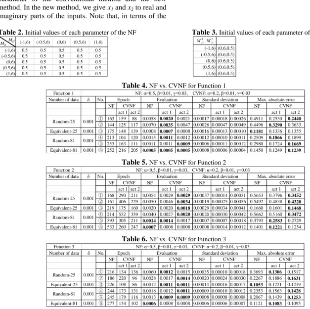
Table 2.Initial values of each parameter of the NF Table 3.Initial values of each parameter of the CVNF

Table 4.NF vs. CVNF for Function 1

(-1,6) (-0.5,6) (0,6) (0.5,6) (1,6) (-1,6) 0.5 0.5 0.5 0.5 0.5 (-0.5,6) 0.5 0.5 0.5 0.5 0.5 (0,6) 0.5 0.5 0.5 0.5 0.5 (0.5,6) 0.5 0.5 0.5 0.5 0.5 (1,6) 0.5 0.5 0.5 0.5 0.5 Mj1 Mj2 (-1,6) (0.6,0.5) (-0.5,6) (0.6,0.5) (0,6) (0.6,0.5) (0.5,6) (0.6,0.5) (1,6) (0.6,0.5) R j M1 I j M1 Function 1

Number of data δ No.

NF NF NF NF

act 1 act 2 act 1 act 2 act 1 act 2 act 1 act 2

① 163 159 88 0.0058 0.0020 0.0021 0.00017 0.00018 0.00026 0.4911 0.2530 0.2440 ② 144 125 117 0.0070 0.0035 0.0047 0.00026 0.00047 0.00049 0.4496 0.3290 0.3633 Equivalent-25 0.001 ③ 175 148 139 0.0008 0.0007 0.0008 0.00016 0.00013 0.00010 0.1181 0.1336 0.1355 ④ 213 104 120 0.0015 0.0011 0.0012 0.00012 0.00010 0.00011 0.2509 0.1866 0.1899 ⑤ 253 163 111 0.0011 0.0011 0.0009 0.00006 0.00011 0.00012 0.2980 0.1724 0.1669 Equivalent-81 0.001 ⑥ 252 216 205 0.0005 0.0005 0.0005 0.00008 0.00006 0.00004 0.1450 0.1249 0.1239 NF: α=0.5, β=0.01, γ=0.03, CVNF: α=0.2, β=0.01, γ=0.03

Epoch Evaluation Standard deviation Max. absolute error

0.001

CVNF CVNF CVNF CVNF

Random-81 0.001 Random-25

Function 2

NF NF NF NF

① 168 290 211 0.0054 0.0029 0.0029 0.00037 0.00014 0.00031 0.5653 0.3796 0.3452 ② 161 406 229 0.0050 0.0046 0.0034 0.00019 0.00025 0.00056 0.5492 0.4838 0.4320 Equivalent-25 0.001 ③ 219 175 160 0.0020 0.0020 0.0018 0.00029 0.00034 0.00041 0.1660 0.1601 0.1468 ④ 214 532 359 0.0040 0.0027 0.0020 0.00020 0.00030 0.00042 0.5662 0.5160 0.3472 ⑤ 393 305 211 0.0014 0.0014 0.0017 0.00007 0.00007 0.00018 0.3793 0.2583 0.2729 Equivalent-81 0.001 ⑥ 533 260 247 0.0007 0.0008 0.0008 0.00008 0.00014 0.00012 0.1401 0.1221 0.1254 Random-81 0.001 CVNF CVNF CVNF CVNF Random-25 0.001 NF: α=0.5, β=0.01, γ=0.03, CVNF: α=0.2, β=0.01, γ=0.03

Function 3

NF NF NF NF

① 216 134 136 0.0060 0.0012 0.0015 0.00035 0.00010 0.00018 0.3693 0.1306 0.1517 ② 186 220 96 0.0028 0.0017 0.0014 0.00020 0.00024 0.00030 0.2267 0.1886 0.1631 Equivalent-25 0.001 ③ 226 108 86 0.0012 0.0011 0.0011 0.00014 0.00016 0.00017 0.1053 0.1221 0.1219 ④ 244 173 131 0.0018 0.0012 0.0011 0.00009 0.00010 0.00012 0.2353 0.1563 0.1428 ⑤ 245 179 116 0.0013 0.0009 0.0009 0.00008 0.00008 0.00008 0.2067 0.1439 0.1253 Equivalent-81 0.001 ⑥ 277 154 102 0.0006 0.0008 0.0008 0.00006 0.00006 0.00007 0.1121 0.1083 0.1095 NF: α=0.5, β=0.01, γ=0.03, CVNF: α=0.2, β=0.01, γ=0.03

Random-25 0.001

CVNF CVNF CVNF CVNF

(5)

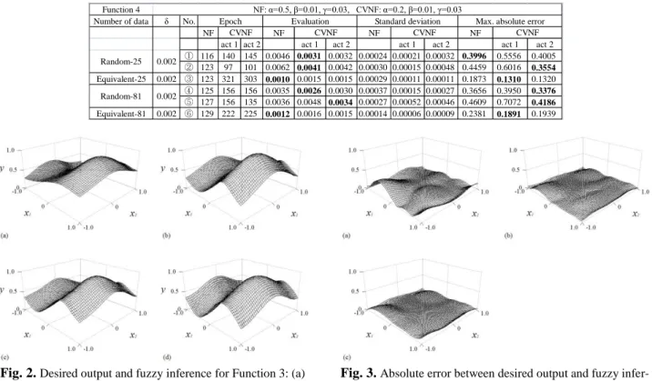
Fig. 2.Desired output and fuzzy inference for Function 3: (a) NF. (b) CVNF using the activation function 1. (c) CVNF using

the activation function 2. (d) Desired output for Function 3.

Fig. 3.Absolute error between desired output and fuzzy infer-ence for Function 1: (a) NF. (b) CVNF using the activation

function 1. (c) CVNF using the activation function 2.

The estimation error is given as follows. First, we per-form learning each fuzzy rule by the conventional method and the new method. Second, we input 2601 estimation data (where both ranges of x1 and x2 are increments of 0.04 from -1 to 1) for Functions 1 and 2 to each learned fuzzy rule. Finally, we get the mean squared error between its output and the desired output for Functions 1, 2, 3 and 4. This is the estimation error. As an example, using the random data 1 (shown in Table 8) in Table 6, we generated each fuzzy rule for the con-ventional method and the new method. Fig. 2 (a), (b) and (c) are each result of the fuzzy inference for 2601 estimation data. Fig. 2 (d) is the desired output of Func-tion 3. Further, Fig. 3 (a), (b) and (c) shows the absolute error between each result of the fuzzy inference and the desired output.

Table 8. Random data 1 in Table 6

From Fig. 2 and 3, compared with the new method, the conventional method could not interpolate around the range in Fig. 3 (a). Further, the new method could fit to such random training sets.

4. DISCUSSION

By the analysis of the results shown in Tables 4, 5, 6 and 7, we can describe as follows.

(1) In terms of the estimation error, we found that the new method is much better than the conventional meth-od for four functions. In particular, the estimation error for random training sets showed good result for all func-tions. Thus, we can say that although the freedom of parameters is limited, the new method could fit for training sets well.

(2) In terms of the absolute error, for Function 1, 2 and 3, the new method showed better results than the conven-tional method. For Function 4, the convenconven-tional method is better than the new method that uses the activation function 1, while it is worse than the new method using the activation function 2. Thus, the new method may or may not be better depending on form of the activation function. For this reason, if we use this method for a model that generates real-valued output for com-plex-valued inputs, we need to change the activation functions depending on the problem to apply.

From the above results of the simulation, we can con-clude that the new method has equivalent to or better accuracy than the conventional method. Furthermore, the new method has a feature that while the parameters have less flexibility, it can fit for training sets well. Therefore, we can say that the new method is a useful tool for learning the fuzzy system model.

Function 4

NF NF NF NF

① 116 140 145 0.0046 0.0031 0.0032 0.00024 0.00021 0.00032 0.3996 0.5556 0.4005 ② 123 97 101 0.0062 0.0041 0.0042 0.00030 0.00015 0.00048 0.4459 0.6016 0.3554 Equivalent-25 0.002 ③ 123 321 303 0.0010 0.0015 0.0015 0.00029 0.00011 0.00011 0.1873 0.1310 0.1320 ④ 125 156 156 0.0035 0.0026 0.0030 0.00037 0.00015 0.00027 0.3656 0.3950 0.3376 ⑤ 127 156 135 0.0036 0.0048 0.0034 0.00027 0.00052 0.00046 0.4609 0.7072 0.4186 Equivalent-81 0.002 ⑥ 129 222 225 0.0012 0.0016 0.0015 0.00014 0.00006 0.00009 0.2381 0.1891 0.1939 Random-81 0.002 Random-25 0.002 CVNF CVNF CVNF CVNF NF: α=0.5, β=0.01, γ=0.03, CVNF: α=0.2, β=0.01, γ=0.03

No. x1 x2 No. x1 x2 No. x1 x2 No. x1 x2

1 0.32 0.92 8 0.4 0 15 -0.04 -0.44 22 0.04 -0.32 2 0.84 0 9 0.32 -0.52 16 -0.96 -0.48 23 -0.08 -0.36 3 0.44 0.4 10 0.36 -0.52 17 0.28 0.44 24 0.64 0.48 4 -0.64 0.52 11 0.84 0.84 18 0.84 -0.4 25 -0.36 -0.16 5 -0.48 0.76 12 -1 -0.36 19 -0.52 0.92 6 -0.88 -1 13 -0.88 -0.12 20 0.96 -0.04 7 -0.04 0.04 14 -1 -1 21 -0.76 0.04

(6)

5. SUMMARY

In this paper, we proposed the new method extending the conventional method to the complex domain for tuning fuzzy rules. Then, we gave the general formulas for this algorithm under Gaussian type membership functions. Finally, in several function identification problems, we showed that the new method outperforms the conventional approach for learning a fuzzy system model.

In the future, we want to show the effectiveness of the proposed method in the subject that can be represented by complex numbers such as image and audio data. The proposed method, by changing a part of it, can also use complex-valued outputs. Further, recently, Neuro-Fuzzy system that has inputs and outputs of complex-number has been proposed [24 - 27]. These methods were pro-posed in different approach from ours. Thus, when we apply our method to the problem of complex numbers, we want to compare with these methods.

Acknowledgements

Supported by grants to KM from the Japanese Society for Promotion of Sciences and the University of Fukui.

REFERENCES:

[1] Ichihashi, H.: Iterative fuzzy modeling and a hier-archical network. In: Proceedings of the Fourth IFSA Congress, Vol. Engineering, Brussels (1991) 49-52 [2] Wang, L. X., Mendel, J. M.: Back-propagation

fuzzy system as nonlinear dynamic system identifiers. In: Proceedings of IEEE International Conference on Fuzzy Systems (1992) 1409-1418

[3] Shi, Y., Mizumoto, M., Yubazaki, N., & Otani, M.: A method of fuzzy rules generation based on neuro-fuzzy learning algorithm. J. Jpn Soc. Fuzzy Theory Systems, 8 (4) (1996) 695–705

[4] Shi, Y., Mizumoto, M., Yubazaki, N., & Otani, M.: A learning algorithm for tuning fuzzy rules based on the gradient descent method. In: Proceedings of the Fifth IEEE International Conference on Fuzzy Systems (1996) 55-61 [5] Angelov, P. P., Buswell, R. A.: Automatic genera-tion of fuzzy rule-based models from data by genetic al-gorithms. Information Sciences 150 (1) (2003) 17-31 [6] Shi, Y., Mizumoto, M.: Some considerations on

conventional neuro-fuzzy learning algorithms by gradient descent method. Fuzzy Sets and Systems 112 (1) (2000) 51-63

[7] Çaydaş, U., Hasçalık, A., & Ekici, S.: An adaptive neuro-fuzzy inference system (ANFIS) model for wire-EDM, Expert Systems with Applications 36 (3) (2009) 6135-6139

[8] Kisi, O., Haktanir, T., Ardiclioglu, M., Ozturk, O., Yalcin, E., & Uludag, S.: Adaptive neuro-fuzzy computing technique for suspended sediment estimation. Advances in Engineering Software 40 (6) (2009) 438-444

[9] Li, J.N., Yi, J.Q., Zhao, D.B., & Xi, G.C.: A new fuzzy identification approach for complex systems based on neural-fuzzy inference network. Acta Automatica Sinica 32 (2006) 695-730

[10] Melin, P., Castillo, O.: Intelligent control of a step-ping motor drive using an adaptive neuro–fuzzy inference system. Information Sciences 170 (2) (2005) 133-151 [11] Turkmen, I., Guney, K.: Genetic tracker with

adap-tive neuro-fuzzy inference system for multiple target tracking. Expert Systems with Applications 35 (4) (2008) 1657-1667

[12] Wang, X., Yang, S. X.: A neuro-fuzzy approach to obstacle avoidance of a nonholonomic Mobile Robot. In: Proceedings of 2003 IEEE/ASME International Confer-ence on Advanced Intelligent Mechatronics (2003) 29-34 [13] Yu, W., Li, X.: Fuzzy identification using fuzzy

neural networks with stable learning algorithms. IEEE Transactions on Fuzzy Systems 12 (3) (2004) 411-420 [14] Shi, Y., Mizumoto, M.: A new approach of

neuro-fuzzy learning algorithm for tuning fuzzy rules. Fuzzy sets and systems 112 (1) (2000) 99-116 [15] Wu, W., Li, L., Yang, J., & Liu, Y.: A modified

gradient-based neuro-fuzzy learning algorithm and its convergence. Information Sciences 180 (9) (2010) 1630-1642

[16] Hecht-Nielsen, R.: Theory of the backpropagation neural network. In: Proceedings of International Joint Conference on Neural Networks (1989) 593-605

[17] Nitta, T.: An extension of the back-propagation algorithm to complex numbers. Neural Networks 10 (8) (1997) 1391-1415

[18] Georgiou, G. M., Koutsougeras, C.: Complex do-main backpropagation. IEEE Transactions on Circuits and Systems II: Analog and Digital Signal Processing 39 (5) (1992) 330-334

[19] Hirose, A.: Complex-valued neural networks (Studies in Computational Intelligence). Springer (2006) [20] Hirose, A.: Complex-valued neural networks:

The-ories and Applications (Series on Innovative Intelligence, 5). World Scientific Publishing Company (2004)

[21] Nitta, T.: Three-dimensional vector valued neural network and its generalization ability. Neural Information Processing–Letters and Reviews 10 (10) (2006) 237-242 [22] Amin, M. F., Murase, K.: Single-layered

com-plex-valued neural network for real-valued classification problems. Neurocomputing 72 (4) (2009) 945-955 [23] Amin, M. F., Islam, M. M., & Murase, K.:

Ensem-ble of single-layered complex-valued neural networks for classification tasks. Neurocomputing 72 (10) (2009) 2227-2234

[24] Subramanian, K., Savitha, R., & Suresh, S.: A Complex-Valued Neuro-Fuzzy Inference System and its Learning Mechanism. Neurocomputing (2013)

[25] Li, C., Wu, T., & Chan, F. T.: Self-learning complex neuro-fuzzy system with complex fuzzy sets and its ap-plication to adaptive image noise cancel-ing.Neurocomputing 94 (2012) 121-139

[26] Li, C., & Chiang, T. W.: Complex neuro-fuzzy self-learning approach to function approximation. In Intelligent Information and Database Systems. Springer Berlin Heidelberg (2010) 289-299

[27] Li, C., Chiang, T. W., & Yeh, L. C.: A novel self-organizing complex neuro-fuzzy approach to the problem of time series forecasting. Neurocomputing (2012)