University of Arkansas, Fayetteville
ScholarWorks@UARK
Theses and Dissertations5-2016
Measuring Teacher Effectiveness: A Comparison
across VA Models Utilizing Arkansas Data
Kelli Lane Blackford
University of Arkansas, Fayetteville
Follow this and additional works at:http://scholarworks.uark.edu/etd Part of theEducational Assessment, Evaluation, and Research Commons
This Dissertation is brought to you for free and open access by ScholarWorks@UARK. It has been accepted for inclusion in Theses and Dissertations by an authorized administrator of ScholarWorks@UARK. For more information, please [email protected].
Recommended Citation
Blackford, Kelli Lane, "Measuring Teacher Effectiveness: A Comparison across VA Models Utilizing Arkansas Data" (2016).Theses and Dissertations. 1545.
Measuring Teacher Effectiveness: A Comparison across VA Models Utilizing Arkansas Data A dissertation submitted in partial fulfillment
of the requirements for the degree of
Doctor of Philosophy in Educational Statistics and Research Methodology
by
Kelli Lane Blackford Pittsburg State University Bachelor of Science in Education, 2004
Pittsburg State University
Master of Science in Mathematics, 2008
May 2016 University of Arkansas
This dissertation is approved for recommendation to the Graduate Council.
____________________________________ Dr. Charles Stegman Dissertation Directors ____________________________________ Dr. Sean Mulvenon Dissertation Directors ________________________________________ Dr. Wen-Juo Lo Committee Member
ABSTRACT
A shift in accountability systems from No Child Left Behind to a reauthorization of the Elementary and Secondary Education Act redefined the mandate of classroom teachers from being highly qualified to highly effective. Whereas previously, a teacher was deemed highly qualified for having a bachelor’s degree, full state certification, and demonstrated knowledge of subject matter in the field they teach, a highly effective teacher had to demonstrate their abilities to move a student at an acceptable rate of student growth (one grade level in an academic year). To provide this evidence, student assessment data was now going to be a part of evaluating a teacher’s effectiveness.
A key concern now, was how to incorporate student assessment data to accurately, determine the input a teacher has had on a student’s learning progress. To address this inclusion, several statistical models have been developed/adapted to parse out the educational contribution of a teacher in a given year. These different models, however, are different in scope in regards to transparency, expense, and data requirements to name a few.
The present study used a cohort of fifth grade math teachers in Arkansas to compare four models (Gains Score Model, Covariate Model, Layered Model, and Equipercentile Model) on their consistency in ranking teachers according to each’s calculations of teacher effects. The teacher rankings were compared to investigate whether or not the teachers had similar rankings across the different models, across time, and for different subpopulations. Results are intended to assist school leaders identify the most transparent, and fiscally responsible model that will best serve their schools’ needs.
©2016 by Kelli Blackford All Rights Reserved
ACKNOWLEDGMENTS
The completion of this degree would not have been possible without the support, guidance and understanding of instrumental people in my life. I would like to thank my chairs, Dr. Charles Stegman and Dr. Sean Mulvenon, who provided the support and encouragement needed for me to persevere and complete the requirements when I got discouraged and wanted to quit. I would also like to thank Dr. Wen Juo Lo for providing me with excellent feedback and support.
My experience at the University of Arkansas provided me the opportunity to work with some amazing people who forged the way for me, specifically, Dr. Denise Airola and Dr. Jam Khojasteh. Thank you both for the support and encouragement you provided while showing me it could be done. And other past and current colleagues at the University of Arkansas; those who continually had faith in me even when I did not. Thank you Kyle Cowan, Randy Prince, Erin Doyle, and Santhosh Anand. And a very special thanks to Jennifer Williams for your motivation, encouragement and sympathetic ear.
My acknowledgements would not be complete without thanking my family. Erv and LeeAnn Langan, you taught me perseverance and to have faith in myself. These qualities were fundamental to my success. Finally, thank you Aaron Blackford. This was an arduous journey through which you never gave up faith in me.
DEDICATION
I would like to thank God for giving me the patience and perseverance to complete this process. Most of all, I would like to dedicate this work to past, present and future teachers. It is our mission to inspire the greatness we will see tomorrow. As teachers, we must stand on the shoulders of many; the shoulders of those who came before us. For it is through learning from their triumphs and failures that helps make us better teachers.
TABLE OF CONTENTS
LIST OF FIGURES LIST OF TABLES
Chapter 1: Introduction 1
Value-Added Analysis ... 6
Statement of the Problem ... 8
Purpose of the Study ... 8
General Research Questions ... 10
Research question 1 ... 10
Research question 3 ... 11
Significance of the Study ... 11
Chapter 2: Literature Review 13
Overview of VAM ... 22
Gain Score Model ... 25
Covariate Adjusted Model ... 28
Layered Model ... 31
Student Equipercentile Model... 33
Conclusion ... 38 Chapter 3: Methods 40 Participants ... 40 Data. ... 43 Testing Instrument ... 45 Procedures ... 48 Validity ... 49 Content-related evidence. ... 50
Evidence of internal structure ... 50
Reliability ... 52
Internal consistency ... 52
Standard Error of Measurement (SEM). ... 53
The Models ... 53
Gain Score Model (GM) ... 53
Covariate Adjusted Model (CM) ... 55
Layered Model (LM) ... 60
Estimating teacher effects. ... 61
Student Equipercentile Model (EM) ... 64
Addressing Research Questions ... 69
Kendall’s coefficient of concordance. ... 70
Chapter 4: Results 73
Model Assumptions ... 73
Stability across Models ... 90
Stability of Models over Time ... 103
Stability of Models across Subpopulations ... 123
Chapter 5: Discussion 152 Models... 155 Measure ... 158 Research Questions ... 160 Research question 1 ... 160 Research question 2 ... 160 Research question 3 ... 160
Rankings Across Models ... 161
Rankings Over Time ... 164
Stability of Models across Subpopulations ... 165
Addressing Concerns ... 166 Future Research ... 168 Final Thoughts ... 169 Bibliography 171 Appendix A 176 Appendix B 184 Appendix C 196 Appendix D 226 Appendix E 256 Appendix F 286 Appendix G 299
LIST OF FIGURES
Figure 1-1. Scale Score predictions for two students with the same prior years’ scores where
students differ on race. 4
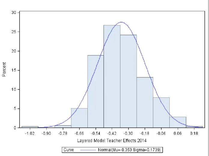
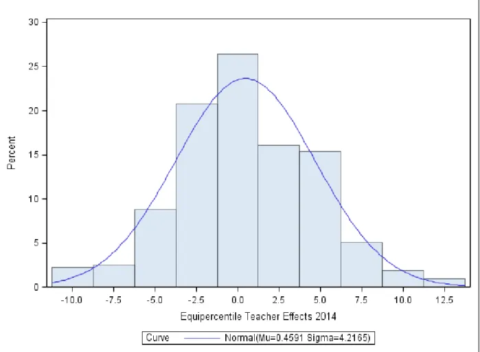
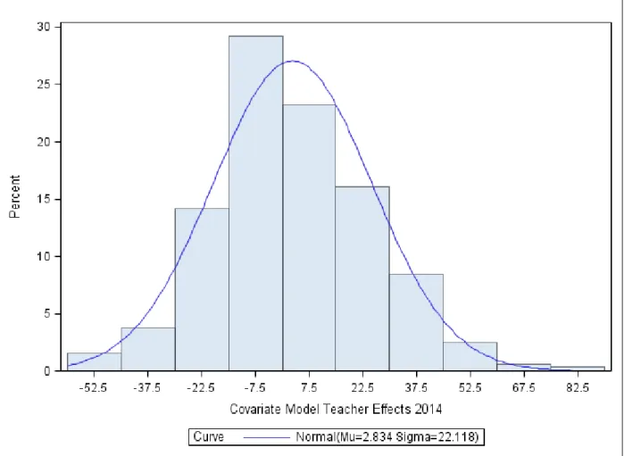
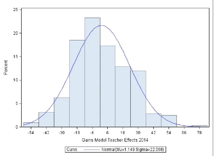
Figure 2-1. Example Student Growth Trajectory 20 Figure 2-2. Example of students with very little difference in rates of change. 28 Figure 3-1. Comparison of errors with and without inclusion of covariates 57 Figure 4-1. 2014 Distribution of teacher effects calculated by the Layered Model. 74 Figure 4-2. 2014 Distribution of teacher effects calculated by the Equipercentile Model. 75 Figure 4-3. 2014 Distribution of teacher effects calculated by the Covariate Model. 76 Figure 4-4. 2014 Distribution of teacher effects calculated by the Gains Model. 77 Figure 4-5. 2014 Relationship between 2014 teacher effects produced by the Covariate Model
and those produced by the Equipercentile Model. 78 Figure 4-6. 2014 Residuals of Teacher Rank by Equipercentile Model predicted from Teacher
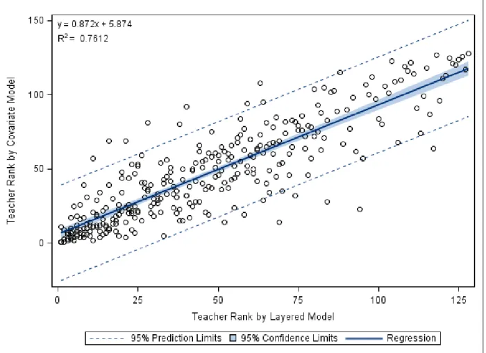
Rank by Covariate Model. 79 Figure 4-7. 2014 Relationship between 2014 teacher effects produced by the Covariate Model
and those produced by the Layered Model. 80 Figure 4-8. 2014 Residuals of Teacher Rank by Layered Model predicted from Teacher Rank by
Covariate Model. 81
Figure 4-9. 2014 Relationship between 2014 teacher ranks produced by the Covariate Model and those produced by the Gains Model. 82 Figure 4-10. 2014 Residuals of Teacher Rank by Gains Model predicted from Teacher Rank by
Covariate Model. 83
Figure 4-11. 2014 Relationship between 2014 teacher effects produced by the Layered Model and those produced by the Equipercentile Model. 84 Figure 4-12. 2014 Residuals of Teacher Rank by Equipercentile Model predicted from Teacher
Rank by Layered Model. 85
Figure 4-13. 2014 Relationship between 2014 teacher effects produced by the Layered Model and those produced by the Gains Model. 86
Figure 4-14. 2014 Residuals of Teacher Rank by Gains Model predicted from Teacher Rank by
Layered Model. 87
Figure 4-15. 2014 Relationship between 2014 teacher effects produced by the Equipercentile Model and those produced by the Gains Model. 88 Figure 4-16. 2014 Residuals of Teacher Rank by Gains Model predicted from Teacher Rank by
Equipercentile Model. 89
Figure 4-17. Cut points for teacher classification and percentage expected in each classification as per the normal distribution. 93 Figure A-5-1. 2012 Distribution of teacher effects calculated by the Layered Model. 176 Figure A-5-2. 2012 Distribution of teacher effects calculated by the Equipercentile Model. 177 Figure A-5-3. 2012 Distribution of teacher effects calculated by the Covariate Model. 178 Figure A-5-4. 2012 Distribution of teacher effects calculated by the Gains Model. 179 Figure A-5-5. 2013 Distribution of teacher effects calculated by the Layered Model. 180 Figure A-5-6. 2013 Distribution of teacher effects calculated by the Equipercentile Model. 181 Figure A-5-7. 2013 Distribution of teacher effects calculated by the Covariate Model. 182 Figure A-5-8. 2013 Distribution of teacher effects calculated by the Gains Model. 183 Figure B-5-10. 2012 Residuals of Teacher Rank by Equipercentile Model predicted from
Teacher Rank by Covariate Model. 184 Figure 5-11. 2012 Region 2 Residuals of Teacher Rank by Equipercentile Model predicted from
LIST OF TABLES
Table Page
1-1. Poverty Classificaiton ... 11
2-1. Student Literacy Achievement Information ... 18
2-2. Student mathematics Achievement Information ... 19
2-3. Comparison Among Value-Added Models ... 37
3-1. Number (Percentage) of Fifth Grade Student Race Demographics by Region, 2014 ... 41
3-2. Number and Percentage of Fifth Grade Students Lunch Status by Region and State ... 42
3-3. Number of Students and Teachers in Each Cohort Across Three Years ... 45
3-4. Test Blueprints for Arkansas Grade 5 Bendhmark Examinaitons from 2012-2014... 47
3-5. Correlation of Mathematics Strands for Grade 3, 2012 ... 51
3-6. Correlation of Mathematics Strands for Grade 4, 2013 ... 51
3-7. Correlation of Mathematics Strands for Grade 5, 2014 ... 52
3-8. Strength for Spearman’s (rho) Correlation Coefficient ... 72
4-1. Normality Statistics for 2014 ... 73
4-2. Spearman’s (rho) Correlations (Kendall’s tau) of Rank Orders Between Models from 2012 to 2014 ... 91
4-3. Teacher Classification Percentages (Frequencies) ... 95
4-4. Fleiss’ Kappa Benchmark Scale ... 96
4-5. Teacher Effectiveness Classification Consistency between Layered Model and Gains Model for 2014 ... 97
4-6. Teacher Effectiveness Classification Consistency between Layered Model and Equipercentile Model for 2014 ... 98
4-7. Teacher Effectiveness Classification Consistency between Gains Model and Equipercentile Model for 2014 ... 99
4-8. Teacher Effectiveness Classification Consistency between Layered Model and Covariate Model for 2014 ... 100 4-9. Teacher Effectiveness Classification Consistency between Covariate Model and Gains
Model for 2014 ... 101 4-10. Teacher Effectiveness Classification Consistency between Equipercentile Model and
Covariate Model for 2014 ... 102 4-11. Spearman’s (rho) Correlations (Kendall’s tau) of Rank Orders within the Covariate Model
From 2012 to 2014 ... 103 4-12. Spearman’s (rho) Correlations (Kendall’s tau) of Rank Orders within the Layered Model
From 2012 to 2014 ... 104 4-13. Spearman’s (rho) Correlations (Kendall’s tau) of Rank Orders within the Gains Model
From 2012 to 2014 ... 104 4-14 Spearman’s (rho) Correlations (Kendall’s tau) of Rank Orders within the Equipercentile
Model From 2012 to 2014 ... 105 4-15. Teacher Effectiveness Classificaiton Consistency for the Covariate Model between 2012
and 2013 across All Regions... 106 4-16. Teacher Effectiveness Classificaiton Consistency for the Covariate Model between 2012
and 2014 across All Regions... 107 4-17 Teacher Effectiveness Classificaiton Consistency for the Covariate Model between 2013
and 2014 across All Regions... 108 4-18. Teacher Effectiveness Classificaiton Consistency for the Layered Model between 2012 and 2013 across All Regions ... 109 4-19. Teacher Effectiveness Classificaiton Consistency for the Layered Model between 2012 and 2014 across All Regions ... 110 4-20. Teacher Effectiveness Classificaiton Consistency for the Layered Model between 2013 and 2014 across All Regions ... 112 4-21. Teacher Effectiveness Classificaiton Consistency for the Gains Model between 2012 and
2013 across All Regions ... 113 4-22. Teacher Effectiveness Classificaiton Consistency for the Gains Model between 2012 and
4-23. Teacher Effectiveness Classificaiton Consistency for the Gains Model between 2013 and 2014 across All Regions ... 116 4-24. Teacher Effectiveness Classificaiton Consistency for the Equipercentile Model between
2012 and 2013 across All Regions... 117 4-25. Teacher Effectiveness Classificaiton Consistency for the Equipercentile Model between
2012 and 2014 across All Regions... 118 4-26. Teacher Effectiveness Classificaiton Consistency for the Equipercentile Model between
2013 and 2014 across All Regions... 119 4-27. Frequency (Percents) of Teachers Consistelntly Classified by Model ... 122 4-28. 2012 Spearman’s (rho) Correlations (Kendall’s tau) of Teacher Ranks by Models by
Poverty Status ... 123 4-29. 2013 Spearman’s (rho) Correlations (Kendall’s tau) of Teacher Ranks by Models by
Poverty Status ... 126 4-30. 2014 Spearman’s (rho) Correlations (Kendall’s tau) of Teacher Ranks by Models by
Poverty Status ... 128 4-31. 2012 Spearman’s (rho) Correlations (Kendall’s tau) of Teacher Ranks by Models by
Minority Status... 130 4-32. 2013 Spearman’s (rho) Correlations (Kendall’s tau) of Teacher Ranks by Models by
Minority Status... 132 4-33. 2014 Spearman’s (rho) Correlations (Kendall’s tau) of Teacher Ranks by Models by
Minority Status... 134 4-34. Percentage (Number) of Teachers in Each Poverty and Minority Categorization Across
Years ... 136 4-35. 2012 Percentages (Number) of Teachers Classified as Ineffective-Exemplary by District
Level Categorization of Minority Status across Models... 137 4-36. 2013 Percentages (Number) of Teachers Classified as Ineffective-Exemplary by District
Level Categorization of Minority Status across Models... 138 4-37. 2014 Percentages (Number) of Teachers Classified as Ineffective-Exemplary by District
4-38. 2012 Percentages (Number) of Teachers Classified as Ineffective-Exemplary by District Level Categorization of Poverty Status across Models ... 143 4-39. 2013 Percentages (Number) of Teachers Classified as Ineffective-Exemplary by District
Level Categorization of Poverty Status across Models ... 146 4-40. 2014 Percentages (Number) of Teachers Classified as Ineffective-Exemplary by District
Level Categorization of Poverty Status across Models ... 147 A-1. Normality Statistics for 2012 ... 176 A-2. Normality Statistics for 2013 ... 180 F-1. Teacher Effectiveness Classification Consistency between Covariate Model and Gains
Model for 2012………...………..278 F-2. Teacher Effectiveness Classification Consistency between Equipercentile Model and
Covariate Model for 2012…..………..279 F-3. Teacher Effectiveness Classification Consistency between Layered Model and Covariate
Model 2012………..280 F-4. Teacher Effectiveness Classification Consistency between Gains Model and Equipercentile
Model for 2012………..………..281 F-5. Teacher Effectiveness Classification Consistency between Layered Model and
Equipercentile Model for 2012…..………..282 F-6. Teacher Effectiveness Classification Consistency between Layered Model and Gains Model 2012………..283 F-7. Teacher Effectiveness Classification Consistency between Covariate Model and Gains
Model for 2013………...………..285 F-8. Teacher Effectiveness Classification Consistency between Equipercentile Model and
Covariate Model for 2013…..………..286 F-9. Teacher Effectiveness Classification Consistency between Layered Model and Covariate
Model 2013………..287 F-10. Teacher Effectiveness Classification Consistency between Gains Model and Equipercentile
Model for 2013………...………..………..288 F-11. Teacher Effectiveness Classification Consistency between Layered Model and
F-12. Teacher Effectiveness Classification Consistency between Layered Model and Gains Model 2013………..290
Chapter 1: Introduction
In January 2002, the No Child Left Behind Act (NCLB) of 2001 was passed into law (Public Law 107-110). NCLB supports standards-based education reform on the principle that attaining high standards and achieving measurable goals can improve individual outcomes in education. This Act required States develop and administer assessments of basic skills to all students enrolled at select grade levels and/or select classes. Administration of these assessments is required for a state to receive federal school funding. Additionally, States were required to establish set measureable objectives created to improve achievement by all students with the end goal of all students at or above the proficient level by the end of the 2013-2014 school year.
During the first nine years of implementation, states sanctioned schools if they failed to meet the targeted percent proficient for a school year as they worked toward the 2014 goal. Further, this measure was based on whether their students were performing at grade level as measured by the respective state Criterion Referenced Test (CRT).
In 2009 President Barack Obama and Secretary of Education Arne Duncan announced a contest among states to spur innovation and reform in our nation’s failing educational systems. This competitive contest was known as Race to the Top (RTTT). RTTT was part of the
American Recovery and Reinvestment Act (ARRA, P.L. 111-5) designed to distribute $4.35 billion dollars for public education to individual states. The RTTT was open to all states that did not have state-level barriers in place that limited the linking of students to teachers or principals for the purpose of evaluation (RTT TA Network Working, 2011). The contest called for states to submit proposals with plans on how they implement comprehensive reforms across four specific areas. The four key areas were:
adopting standards and assessments that prepare students to succeed in college and the workplace and to compete in the global economy;
recruiting, developing, rewarding and retaining effective teachers and principals, especially where they are needed most;
building data systems that measure student success and inform teachers and principals how they can improve their instructional practices; and
turning around the lowest-performing schools.
Not dissimilar from the original goals of NCLB, the overarching goals of RTTT are to drive substantial gains in student achievement, improve high school graduation rates and college enrollment, and narrow achievement gaps between subpopulations. An instrumental component of RTTT was the call to have effective teachers in all schools; the spot light that had been aimed solely at student achievement as measured by the state CRT, was now aimed at how effectively teachers were in educating their students.
In 2002, NCLB called for all schools to employ “highly qualified teachers (HQT)” in “core academic subjects” by the end of the 2005-2006 school year. Individual states were allowed to define HQT, and most defined HQT as having a bachelor’s degree, full state certification, and demonstrated knowledge of subject matter in the field they teach. Under this program most teachers were defined as HQT. Through RTTT the requirement of “highly qualified” teacher was replaced with “highly effective” teacher. RTTT defined an effective teacher as one “whose students achieve acceptable rates (e.g. at least one grade level in an academic year) of student growth (as defined in this notice).” It is clear the intent was in order for teachers to be effective, student learning and outcomes are increased “at or above what is expected within a typical school year” (Lomax & Kuenzi, 2012). In effect, a significant component of RTTT was that teacher evaluations must be based on student growth.
(in theory, an effective teacher will have this outcome). However, the teacher is not the only influence on student achievement. There are numerous confounding variables that may contribute positively or negatively to student outcomes (Hanushek, Kain, O’Brien, & Rivkin, 2005; Lomax & Kuenzi, 2012). For example, in addition to the effects of instruction, student learning may be influenced by the school and school policies, the school and district
administration, peer-to-peer interaction, parental involvement, and accessible resources. Moreover, external factors outside the school setting, such as individual past experiences,
socioeconomic status, disability status, the community, etc. may also affect student learning. Due to the interwoven contributions of all sources, it makes it difficult to parse out what knowledge can be directly attributed to teacher input.
In addition to the impact of confounding variables on student achievement, evaluators should address further limitations in measuring teacher effects. Many models in use employ covariates as a way to statistically partition out effects that are beyond the control of the teacher (D. F. McCaffrey, Lockwood, Koretz, Louis, & Hamilton, 2004). Covariates are included into models to eliminate some systematic variance (Ballou, Sanders, & Wright, 2004) and can improve the power of inferential statistics when reliably measured.
Policy makers appear to walk a “thin line” when including covariates such as
participation in the Free or Reduced Lunch Program (FRLP) into any measure of teacher effect. By including FRLP as a covariate, it could be construed that policy makers are assuming that socioeconomic status may influence students’ ability to learn and thus not hold teachers accountable for equitable achievement for students from low socioeconomic backgrounds. However, since students from low socioeconomic backgrounds tend to have lower scores on student assessments compared to students from higher socioeconomic backgrounds (Lomax &
Kuenzi, 2012), it may not be appropriate to exclude socioeconomic status as a covariate when estimating teacher effects. A similar perspective may be taken when considering a student’s race.
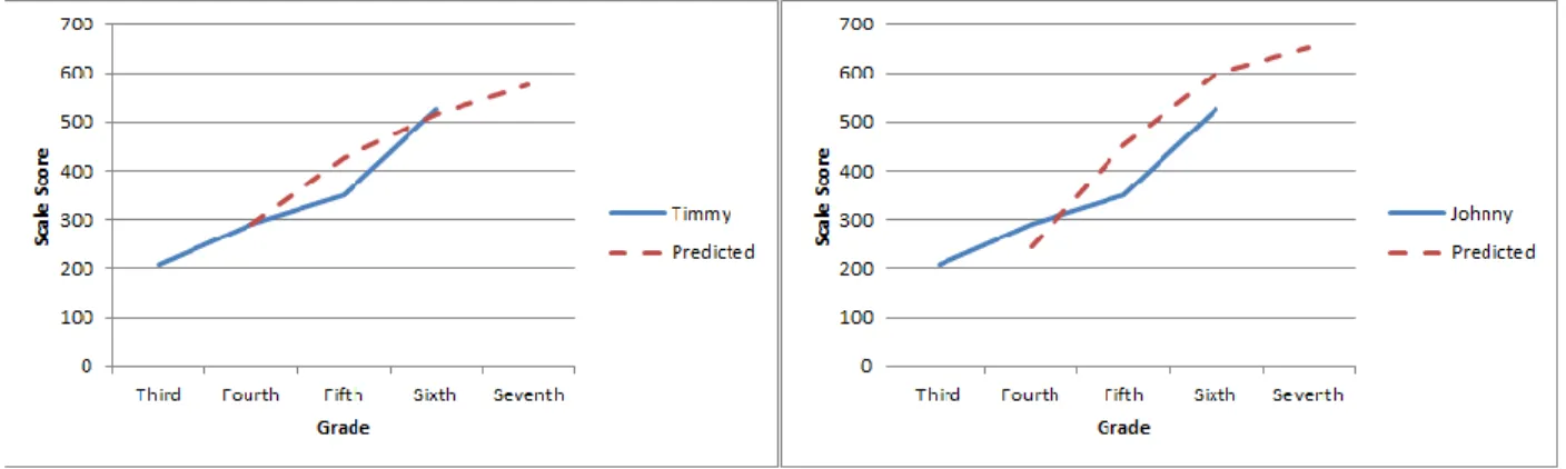
Consider the hypothetical growth trajectories calculated for Johnny and Timmy with the race covariate included in the calculations displayed in Figure 1-1. Johnny and Timmy are seventh grade students from the same school, in the same class. Assume they have the exact same prior end-of-year test scores for third through sixth grades. These two students also have the same poverty classification. The only difference in the two students is race; Timmy is black and Johnny is white. Based on the above information, the following predictions are made for their seventh-grade end-of-year scores.
Figure 1-1. Scale Score predictions for two students with the same prior years’ scores where students differ on race.
The prediction for each student with the covariate of race included in the growth model is that their score will be closer to the average for their race, regression towards the mean. So although both boys have the same test score history, Johnny’s projected score is higher than that of Timmy’s. In essence, because Timmy is black, he is expected to perform lower than Johnny on the seventh grade test. How can one justify that, with everything equal (prior test score history, poverty level, classroom teacher, etc.) the white student is expected to perform higher than the black student. In this effect, are we to assume Timmy have less growth than Johnny based on race alone?
Putting this in terms of measures of teacher effects, when both boys again have the same score on the seventh grade exam, since Jonny’s achievement gains is below that of what was expected, he will count negatively towards the teacher’s effectiveness measure. But since
Timmy’s measure exceeded the expectation set for him, he will contribute positively towards the teacher’s effectiveness measure.
A valid comparison cohort for use in estimating a teacher’s instructional effect on student achievement will assist researchers identify the teacher effect. One approach, as is current in practice (Lomax & Kuenzi, 2012), is to compare a teacher’s effect as calculated via a statistical model against that of the average estimated teacher effect in a school, district or state. Of importance is identifying the standard by which you wish to measure your teacher effect estimates. If the goal is to provide information about a teacher’s effectiveness relative to others in the district, then producing estimates relative to the average teacher in the district would be appropriate.
Researchers have been studying different ways in which to measure the impact a teacher has on student learning, the teacher effect. In current practice among states, there exist different modes of evaluating teacher effectiveness spanning classroom observations, classroom
walkthroughs, interviews and statistical models linking student achievement to teachers.
Common statistical models currently in practice to measure teacher effects include Value-Added models, growth models, and status models (Ligon, 2008). This study investigates the different inferences on teacher effectiveness that can be derived from three Value-Added models and one Growth model.
Value-Added Analysis
Value-added analysis is a statistical technique that measures student academic growth over time (“Understanding Value-Added”, n.d.); the impact a teacher, school, or district has on the amount of progress a student makes during the course of a school year (Tennessee Value Added Assessment System segment 1.1 Overview video team-tn.org/teacher-model). This methodology can be used to measure teacher and/or school impacts on student learning parsing out effects of other contributing factors (The Teacher Advancement Program, n.d.). Several studies have determined that the teacher is the largest contributor to a child’s education among all other variables (George, Hoxby, Reyes, & Welch, 2005; Wright, Horn, & Sanders, 1997).
As the teacher is the largest contributor to a child’s education according to researchers, it is pertinent that our classrooms are staffed with effective teachers. Determining what constitutes an effective teacher has been subject to debate. With the adoption of NCLB, and more recently RTTT, there has been a greater push in requiring student standardized test scores be a component of a teacher’s effectiveness rating. The United States Department of Education (DOE) has
identified four different types of models currently in use by different states to measure teacher effects utilizing student achievement. These models include the Gain Score Model (GM), Covariate Adjusted Model (CM), Layered Model (LM) and Equipercentile Model (EM).
However, depending on the statistical model chosen, results may vary for an individual teacher. The conclusions drawn based on the employed model may create potentially eclectic consequences on the evaluation of teachers. Potential consequences include undue promotion or demotion, incorrectly awarding or denying incentive of pay, or incorrectly identifying or failing to identify teachers in need of remediation (Ali & Namaghi, 2010; Harris & Rutledge, 2007). Therefore, analyzing and comparing these four models forms the basis for this research.
The most common statistical methods for providing measures of teacher effectiveness based on student achievement are referred to as Value-Added Models (VAM). However, not every value-added assessment system is a VAM. VAMs are quasi-experimental statistical models that seek to establish a link between a variable (teacher) and an outcome (student achievement) (Lomax & Kuenzi, 2012). Three of the models under investigation in this study (the GM, the CM and the LM) are VAM models. The fourth model under investigation, the EM, is a growth model commonly referred to in the literature as the Student Growth Percentile Model (Betebenner, 2009). VAMs and growth models are not interchangeable. While both measure growth over time, VAMs are a specific type of growth model that aim to identify to what extent can the gains/losses in student achievement be attributed to a specific teacher (Reform Support Network, 2011) and the generic “growth model” is simply an unadjusted case of the VAM (Ligon, 2008); i.e. it does not “control for” the influence of selected factors such as
socioeconomic status. The EM is used to examine changes in the student achievement of an individual student relative to other students. This information is then aggregated to the teacher level to produce a measure of teacher effect (RTT TA Network Working, 2011).
When selecting a model to analyze value-added effects of a teacher, policy makers must think critically about how the results will be used; not every model will produce equally useful information (RTT TA Network Working, 2011). Model selection depends on which decisions the information will be used to make and which model will best provide information for these
decisions. Further, interested persons must be mindful of the cost of the model and the ability of the results to be comprehensible to parents and other educational stakeholders. Additionally, although the RTTT requires student data be used in calculating measures of teacher effects, statisticians have cautioned administrators on the use of statistical models as the sole method for
determining the value-added by a teacher (Braun, 2005; Lissitz, 2012) particularly when high stakes are associated with teacher ratings.
Statement of the Problem
When choosing which statistical model to use to estimate teacher effects, policy makers are faced with several complicated decisions. Some models, like the GM, are easy to compute, understand, are less expensive and do not require multiple years of data. However, the GM does not consider students’ initial achievement level, adjust for background characteristics, and other factors such as measurement error. In contrast, the LM requires several years of data in multiple subject areas, is complex, expensive and difficult to understand. They do, however, provide relatively precise estimations of teacher effects. Additionally, when deciding which model to employ, policy makers must take into consideration the impacts for including/excluding covariates, such as socioeconomic status or race, into models to measure teacher effects.
There are many factors that must be taken into consideration when choosing a statistical model to best estimate teacher effects. Policy makers need to be provided with greater
understanding of the consequences of model selection. The objective here was to choose a model that evaluates a teacher’s effectiveness via measures of teacher effects. I did not seek to predict whether a teacher will be effective with a particular class in a given year, rather I wished to evaluate whether or not their contributions to students was positive; did the students make appropriate learning gains?
Purpose of the Study
It is imperative that K-12 classrooms have effective teachers. A 2012 study by the George Bush Institute found students in the U.S. are not achieving at the same level as their international counterparts (Hoffmann, 2012). In addition, the New Teacher Project reports even
high-need students assigned to a highly effective teacher for three consecutive years may outperform students not taught by a highly effective teacher for three years by as much as 50 percentile points (Weisberg, Sexton, Mulhern, & Keeling, 2009).
The New Teacher Project (2009) suggests student level assessment scores should account for no more than 60% of the total teacher effectiveness score in their blueprint for a “rigorous, fair and credible teacher evaluation systems (“The New Teacher Project,” 2010).” While allowing for other measures to be taken into consideration, such as classroom observations or other student learning measures, the New Teacher Project asserts the most accurate measure of student progress should carry the most weight.
With the emphasis of accountability shifting to teachers and their effectiveness in the classroom, it is important that models will most accurately attribute student gains in achievement to the correct source, thus helping to identify a teacher’s level of effectiveness. And as the
distributions of test scores change every year, it is important to see the differing results and differing conclusions that one could derive about a teacher’s effectiveness based on different statistical models.
For the purpose of this study the Gain Score Model (GM), Covariate Adjusted Model (CM), Layered Model (LM) and Equipercentile Model (EM) will be investigated to compare results for differences in measures of teacher effects across multiple years in Arkansas. More specifically, are the different models producing the same teacher rankings?
The GM is the most parsimonious model under investigation in this study. The GM calculates difference in student scores between two years to see how much gain a student made throughout the school year. The typical GM averages the differences for all students in a
classroom to generate a teacher measure. The teacher measure is compared to the average gain score for a group of teachers (i.e. in a school, in a district, or state).
The CM models current year’s test scores as a function of prior year’s test scores with the inclusion of student and classroom characteristics as covariates. The teacher effect estimates the impact a teacher has had during the current year.
The LM simultaneously models scores across multiple years and multiple subjects. Later years of teacher effects build on earlier estimates, thus providing “layering” effects. Models of this type do not include covariates, such as student socioeconomic level, in the equation.
Finally, the EM model analyzes students’ progress during a school year to peers with similar academic history. This model uses quantile regressions placing current performance relative to prior performance into a percentile metric (RTT TA Network Working, 2011).
General Research Questions
Research has shown that teacher effects vary from class to class, year to year and depending on which statistical model was used in the estimation. Similarly, the choice of statistical model chosen to measure teacher effects could result in different conclusions
pertaining to the amount of added value a teacher has on student achievement. Given interest in quantifying the amount of added value a teacher has to his/her students, the following research questions were developed comparing the four popular models currently in place with actual student data.
Research question 1. Did the rank order of estimates of teacher effects differ depending on the model chosen to measure the teacher effects? To test this question, the rankings of each teacher according to their estimated teacher effectiveness were compared for each model.
demonstrating stability in the models, e.g. a teacher with a gain score rating of 3 in 2013 received a same rating of 3 in 2014? To test this question, correlations of teacher effectiveness ratings were compared within each model.
Research question 3. Did models measuring teacher effects have consistent results for similar teachers regardless of student background characteristics? To test this hypothesis, teachers were categorized by poverty level as measured by the percent of students in the district participating in the Free/Reduced lunch program (high, medium or low poverty) on minority status depending on the percentage of students in the district who were neither White nor Asian. Teachers were ranked within each subpopulation. Their rankings were correlated across models. Table 1-1 shows the distribution of poverty classification across the five regions in Arkansas. Table 1-1 Poverty Classification Frequency (Percent) Region 1 68,182 (58.27%) Region 2 44,272 (66.61%) Region 3 56,520 (56.82%) Region 4 21,729 (67.67%) Region 5 13,725 (72.95%)
Significance of the Study
The ability to evaluate teachers based on student gains is paramount to identifying an important characteristic that make teachers effective. The consequences of ineffective teachers are far reaching. Schools/districts retaining ineffective teachers put students, fellow teachers, and
of ineffective teachers is cumulative and additive. In fact according to their research, teacher sequencing can result in a difference of 50 percentile points in student achievement over the course of three years. And yet while effective teachers receiving students from ineffective teachers can facilitate excellent gains, the residual effects of the ineffective teacher can still be measured in subsequent years (Sanders, Rivers, & Hall, 1996).
This study seeks to identify which statistical model most accurately attributes student gains in achievement to teachers and under what circumstances. By narrowing the selection of statistical models, schools and districts can better expend their resources in selecting a model that will produce the most precise results.
Chapter 2: Literature Review
The No Child Left Behind (NCLB) act of 2001 mandated that all students would be performing on grade level (i.e., 100% proficient) in mathematics and literacy by the school year 2013-2014. To comply with this mandate, each state was permitted to design unique Adequate Yearly Progress (AYP) plans to reach this goal by 2013-2014 (NCLB, 2001 Sec. 1111 [b] [2] [F]). While some states opted for a curvilinear approach with little improvements in the
beginning years followed by significant gains in the culminating years, Arkansas utilized a linear trajectory where steady increases were to be made each year. In the end, Arkansas schools and districts had three means by which they could meet the predetermined Annual Measures of Objectives (AMOs) to be considered as having made AYP. Arkansas schools and districts could meet the AMOs by percent proficient, Safe Harbor or growth for seven subgroups in
mathematics and in literacy. The seven subgroups included: Combined Population, African American, Hispanic, Caucasian, Economically Disadvantaged, Limited English Proficient (LEP) and Students with Disabilities (SWD).
As test scores are the predominant data used in determining a school’s status, it is imperative that scores be comparable across tests and from year-to-year (Lissitz & Huynh, 2003). The use of horizontal scaling of scores and vertical scaling of scores can help ensure that scores are comparable across tests (horizontal scaling) and from year-to-year (vertical scaling). Consider the third-grade end-of-year exam. Assume this exam has 5 versions (Test Form A – Test Form E). Horizontally scaling these tests would take students’ raw scores on the particular exam and transform them to a new set of numbers with a specific selected attributes such as mean and standard deviation. To this end, the purpose of scaling the exams to the selected attributes was to equate all five versions of the third-grade exam; it is now possible to compare
The use of vertical scaling to compare scores from year-to-year is more complicated. This complexity arises from test specifications. When we scale horizontally, third grade Test-Form A to Test-Form B, we know the same set of test specifications was used for the creation of each test; they are testing mastery of the same information. However, when we test from year-to-year, students will be expected to have mastery of more content in the later year than the first, thus, different test specifications. This is a violation of a major assumption needed for equating that the tests are measuring the same general content. By violating this assumption, rather than equating the two tests, you are predicting the second test score from the first test score (i.e., you are using a student’s third-grade test score to predict their fourth-grade test score).
Lissitz & Huynh (2003) purposed the idea of vertical moderation to circumvent the problems that arose from vertical equating. Rather than equating a score on one exam to a score on another exam, vertical moderation focuses on the category of performance attributed to students based on the state assessment (e.g., below basic, basic, proficient, advanced). They argue that the focus of instruction should be that of meeting the achievement level that predicts adequate completion of the next grade. Through a judgmental process of defining the skills necessary to be deemed as having successfully completed the next grade and a statistical process that will project student performance forward, educational agencies are able to predict whether students are likely to gain the required knowledge to be considered as having met the standard (proficient) the next year.
To qualify as having met AYP through percent proficient, each school/district had to have a percentage of students (excluding mobile students) advanced or proficient greater than or equal to the predetermined AMOs for a given year in each subgroup. If a school/district failed to meet or exceed the AMO for any subgroup in either math or literacy, then the school/district
would fail to meet AYP for that year through percent proficient. Percent proficient was calculated using the following formula:
# non-mobile proficient/advanced students All non-mobile students tested
If a school failed to meet AYP through percent proficient, they could then determine if they met the AMOs through Safe Harbor. The state agency provided the formula below:
(100 − 𝑃𝑏) − [(100 − 𝑃𝑏)(0.1)] ≥ (100 − 𝑃𝑎)
where 𝑃𝑏 is the percent of non-mobile students classified as proficient or advanced for the
previous year and 𝑃𝑎 is the percent of non-mobile students classified as proficient or advanced
for the current year to determine whether a school met Safe Harbor. Essentially, a school must decrease their percent of non-mobile students NOT proficient by 10% to be considered to have met Safe Harbor (Mulvenon, 2010). This is calculated for each of the seven subgroups for math and literacy. Each school/district could employ Safe Harbor for each subgroup in both subjects only after their secondary indicators had been met. Secondary indicators will be discussed below.
NCLB offered some flexibility in their measurement models (Mulvenon, 2010). To this end, both the Safe Harbor and percent proficient calculations utilized a confidence interval calculated from the state data which allowed some schools to meet AYP despite being a fraction of a percentage off of the required AMO needed. The required AMOs could be reached by all seven subgroups in math and literacy through a combination of percent proficient and Safe Harbor.
The third measure by which a school/district could meet AYP was through individual student growth. This alternate method to measure student growth is known as the Student Growth Model (GM). Growth models typically refer to models that track student achievement scores from one year to the next in an effort to determine if the student made individual progress
toward being proficient by 8th grade during the course of the school year. Growth models could be considered a subset of VAM as all growth models are VAMs but not every VAM is classified as a growth model (Briggs, Weeks, & Wiley, 2008). Arkansas was one of 11 states selected to implement their growth model (O’Malley et al., 2009).
During the years of investigation for this research, all students in grades 3-8 in Arkansas were administered CRT exams (Benchmark exams) in mathematics and literacy that were scored on a moderated vertical scale (Lissitz, R. & Huynh, H., 2003). A non-linear growth trajectory was calculated for each student from their initial Benchmark score with the expectation that each student will be proficient by the eighth grade and more growth is expected to occur in the earlier years than the later years. The score a student would have to make each year to be on track to being proficient by eighth grade is known as the expected scale score. If a student met their expected scale score for a given year, the student was considered to have “met growth” for that year even if the score was below the proficiency cut score for that grade. In the Arkansas SGM, non-mobile students who were not proficient but “met growth” were added to the numerator when calculating the percent proficient. The formula below was used to calculate growth.
# non-mobile proficient/advanced students + # non-mobile below proficient students who met growth All non-mobile students tested
For a subgroup to meet growth, the growth calculation must meet or exceed the required AMO for the given year. In order to invoke growth to meet AYP, a school must meet the AMO via growth for EVERY subgroup within each subject. Additionally, since a growth trajectory was calculated for each individual student, no confidence intervals applied to the growth model. End of Course (EOC) exams in high school (Algebra, Geometry, Biology and Grade 11 Literacy)
were excluded from growth calculations as they are not measured on a vertical scale or year to year.
Table 2-1 below shows the scaled scores, expected scaled scores, proficiency cut scores and whether or not the three fictitious students met growth for literacy. For Literacy, Mary and John will count in the numerator for the percent proficient calculation as both scaled scores exceed the proficiency cut score. Although Glen failed to reach the proficiency cut score, he did meet his expected scale score and thus all three students will count in the numerator for the growth calculation. Despite not having met her expected scaled score, Mary would still count in the numerator as the growth model is a growth to proficiency model and she was proficient. Also, since the growth model gives credit to students who were not proficient, but met their growth trajectories, each student can count only once in the numerator. Therefore John would only count once in the numerator for his proficient scaled score even though he also met his growth trajectory.
Table 2-1
Student Literacy Achievement Information
Student Grade Literacy Proficiency Classification Literacy Scaled Score Literacy Expected Scaled Score Literacy Proficiency Cut Score Literacy Met Growth Glen Smith 4th Below Basic 325 316 559 Yes Mary Williams 5th Proficient 641 661 604 No John Jones 6th Proficient 698 603 641 Yes
Table 2-2 below shows the scaled scores, expected scaled scores, proficiency cut scores and whether or not the three fictitious students met growth for mathematics. For mathematics, Mary and John will count in the numerator for the percent proficient
calculation as both scaled scores exceed the proficiency cut score. Mary and John are the only two students as well who will count in the numerator for the growth calculation. Glen will not count in either calculation as his mathematics scaled score was below the proficiency cut score and his expected mathematics scaled score. Although Mary failed to meet her expected mathematics scaled score, she will still count in the numerator of the growth calculation since she did exceed the mathematics proficiency cut score.
Table 2-2
Student Mathematics Achievement Information
Student Grade Mathematics Proficiency Classification Mathematics Scaled Score Mathematics Expected Scale Score Mathematics Proficiency Cut Score Mathematics Met Growth
Glen Smith 4th Basic 515 520 559 No Mary Williams 5th Proficient 658 667 604 No John Jones 6th Advanced 785 675 641 Yes
Refer to Figure 2-1 for an example of a student growth trajectory as provided by the National Office on Research,
Measurement and Evaluation Systems (NORMES) to the state agency. The growth trajectory includes proficiency cut scores, expected scores, and student scaled scores. Figure 2-1 shows the expected mathematics growth trajectory and mathematics scaled scores for the above student John. We can see that John exceeded the proficiency cut score for third through sixth grades. We also see that although John was proficient in fifth grade, he failed to meet his expected scaled score. Failing to meet his expected scaled score for fifth grade indicated at that time, he was no longer on target to being proficient by eighth grade.
Figure 2-1. Example Student Growth Trajectory
Each school had two secondary indicators that must additionally have been met in addition to meeting the AMOs for a given year. The first secondary indicator for AYP required an overall school attendance rate of at least 91.13% for the elementary, middle and junior high schools and a graduation goal of 73.9% for high schools. The additional secondary constraint required that every child enrolled in a tested course be tested; each subgroup had to achieve a predetermined percent tested of 95%. By testing every student, the academic achievement of every student would be measured thus providing information to teachers and parents enabling them to provide appropriate remediation to individual students in an effort to ensure that no child was left behind, the intention of NCLB.
In 2009 the federal government announced a new initiative called Race To The Top (RTTT) in which states could revamp their state accountability systems while competing for federal funding. The RTTT initiative mandated one important piece not fully extended in the original NCLB plan: measuring teacher effects, the contribution each teacher has to the academic
400 500 600 700 800 900
Third Fourth Fifth Sixth Seventh Eighth
Proficiency Cut Score Expected Scaled Score Scaled Score
Several studies have concluded that an effective teacher is the most critical school-based factor contributing to student learning (Kane, Rockoff, & Staiger, 2008; Rivkin, Steven,
Hanushek, Eric, Kain, 2005; Wright et al., 1997). The original NCLB of 2001 addressed teacher effectiveness to an extent. It required that all schools would be 100% staffed by highly qualified teachers by the end of the 2005-2006 school year. The federal government loosely defined a highly qualified teacher as:
“To be deemed highly qualified, teachers must have: 1) a bachelor’s degree, 2) full state certification or licensure, and 3) prove that they know each subject they teach” (NCLB Fact Sheet, 2004). A problem with this loose definition was that each state had the prerogative to set their own pass scores on qualifying teacher exams (e.g. PRAXIS).
The RTTT initiative elaborated on the requirement of staffing highly qualified teachers to include teachers not only be highly qualified, but also highly effective (Achieve Inc., 2009). RTTT required states to have viable methods “to measure the effectiveness of teachers, provide an effectiveness rating to each individual teacher, and use those ratings to inform professional development, compensation, promotion, tenure, and dismissal” (Weisberg et al., 2009). Improving teacher quality and effectiveness was identified as one of the most pressing issues facing schools in their efforts for reformation and improvement (Thoonen, Sleegers, Oort,
Peetsma, & Geijsel, 2011). As a result, states were required to include multiple inputs to measure a teacher’s effectiveness with a measure of student growth mandated as one input (Achieve Inc., 2009) in their RTTT application to the federal government. Additionally, funded states were required to develop a large data base to link student achievement and growth data that would connect individual teachers to individual students (Crowe, 2011).
Overview of VAM
The concept of Value-Added Models (VAMs),prevalent for years in econometrics, was originally adopted by William Sanders for use in education in Tennessee and has now expanded to include states such as Ohio and Pennsylvania (Bruan, 2005). Value-added analysis is a methodology used to partition out the effects a teacher or school has had on student learning (The Teacher Advancement Program, n.d.). These models allow researchers to identify true teacher and school effects after controlling for student characteristics and other factors contributing to student achievement (Darling-hammond, Amrein-Beardsley, Hartel, &
Rothestein, 2012). It is important to note that teacher “effects” refer to the output of a statistical measure, in this case, the change in scores as measured by the state CRTs, whereas teacher “effectiveness” refers to the interpretation related to the teacher contribution on student growth (Braun, 2005) that includes other measures beyond student test scores (i.e., interviews,
observations, etc.).
Henry Braun (2005), amongst others (Berk, 2005; Jerald & Van Hook, 2011), cautions measuring a teacher’s effectiveness solely through the use of statistical tests used to measure students’ growth. This is especially of importance when considering high stakes such as salaries, promotions and/or sanctions, are concerned (Hibpshman, 2004). VAM models are inappropriate to be used alone in making these decisions. Braun cautions on the ability of districts and schools to make valid determinations of a teacher’s effectiveness as there are many pitfalls associated with the data typically available to schools and districts. VAM results can, however, be appropriately used to identify teachers in need of assistance, and how to plan and target professional development (Murphy, 2012; Weisberg et al., 2009).
The American Education Research Association and National Academy of Education published a list of qualities effective teaches are said to possess in the republication of Getting Teacher Evaluation Right: A Brief for Policy Makers in 2011. These specific teaching practices are said to promote student gains. Effective teachers are said to:
Understand subject matter deeply and flexibly
Connect what is to be learned to students’ prior knowledge and experience
Create effective platforms and supports for learning
Use instructional strategies that help students draw connections, apply what they’re learning, practice new skills, and monitor their own learning.
Assess student learning continuously and adapt teaching to student needs;
Provide clear standards, constant feedback, and opportunities for revising work; and
Develop and effectively manage a collaborative classroom in which all students have membership
To truly measure the effectiveness of a teacher as defined above, administrators must employ interviews and/or observations in addition to measures of student growth. Given these characteristics of an effective teacher, teacher effectiveness cannot be measured by VAMs alone. VAMs are purely statistical in nature and rely on no measures of student learning other than test outcomes for measuring the effects of a teacher (Braun, 2005). VAMs strictly use student test scores to identify the effect a teacher has had on student growth by measuring year to year change. The authors of VAMs argue that by measuring changes in student test scores from year to year, they are objectively able to isolate impacts specific teachers have had on student learning (Braun, 2005).
As mentioned, for the purpose of measuring teacher effects, the goal of VAMs is to parse out influences on student achievement that are not related to the impact a teacher has had on
effects of school demographics, such as the mean socio-economic status of the school or the racial composition of students zoned to attend certain schools, are referred to as composition effects (Darling-hammond et al., 2012). When the composition of students across teachers differs from the average of the school, there is potential for biased estimation of teacher effects. The environments in which teaching and learning take place constitute the ‘contextual effects’
(Daniel F McCaffrey, Lockwood, Koretz, & Hamilton, 2003). Several models in use, such as the Covariate Adjusted Model and the Layered Model, include variables such as these to help control for potential bias.
There are contextual effects considered to be systematic factors associated with learning for which VAMs cannot control. Some of these factors effecting student learning include: school factors such as class sizes, curriculum materials, and resources; home and community supports or challenges; individual student needs and abilities; peer culture and achievement; and prior teachers and schooling as well as other current teachers (Braun, 2005; Darling-hammond et al., 2012; Rothstein, Haertel, Amrein-Beardsley, Darling-Hammond, & Little, n.d.).
While there exist contextual factors that VAMs are unable to control for, statisticians and policy makers alike would disagree that some factors, such as race or socioeconomic status, should be included as covariates in VAM models. Despite understandings of typical impacts of race or socioeconomic status on a student’s education, it is neither politically nor morally correct to assume that two students starting at the same ability level, with all other factors consistent, less race or socioeconomic status, would have different projected academic trajectories.
For the purpose of this study, teachers will be compared to fellow teachers in their regions. As a result, school factors, home and community support, and peer culture, should be similar for all teachers. Additionally, it is assumed that individual student needs abilities and prior teacher
impacts will be randomly distributed among teachers consequently having no significant impact on one teacher.
As mentioned in 0, four different statistical models commonly used to measure teacher effects are the Gain Score Model (GM), Covariate Adjusted Model (CM), Layered Model (LM) and Equipercentile Model (EM). The general case of each model is described below.
Gain Score Model
The Gain Score Model (GM) measures year-to-year change by subtracting the prior year score from the current year score. Typically, a teacher’s gain score is the average of the gains for all their students in a given year. This score is then compared to the gains of other teachers teaching in similar areas. The GM below as
𝑑𝑖𝑡 = 𝑦𝑖𝑡− 𝑦𝑖,𝑡−1= 𝜇𝑖𝑡+ 𝑇𝑡+ 𝑒𝑖𝑡 (2 - 1) Where
𝑑𝑖𝑡 is the difference between two successive scores for student i at the 𝑡𝑡ℎ year of data collection
𝑦𝑖𝑡 is the score for the 𝑖𝑡ℎ student in the 𝑡𝑡ℎ year of data collection for 𝑡 ≥ 1
𝑦𝑖𝑡−1 is the score for the 𝑖𝑡ℎ student in the 𝑡 − 1𝑡ℎ year of data collection for 𝑡 ≥ 1
𝜇𝑖𝑡 is the student specific mean for grade level at year t
𝑇𝑡 is the teacher effect that estimates the impact the current teacher has on student
academic growth for year t
𝑒𝑖𝑡 is the residual error term for the 𝑖𝑡ℎ student in the 𝑡𝑡ℎ year of data collection that represent the effects unique to student i due to chance that have not been controlled.
This model assumes that for each grade, teacher effect and the residual error terms (𝑒𝑖𝑡) are respectively independent identically distributed (i.i.d.) normal random variables with mean zero, variance 𝜎Tt2 and 𝜎ϵt2, and independent of each other.
The GM is easy to compute/implement and explain. Since the model simply finds the difference in year-to-year scores, time-invariant factors such as poverty, race or gender as well as students’ prior achievement scores beyond one year, do not need to be measured. The GM
requires only two years of data whereas other models can be data intense.
While the ease in calculation and transparency of the GM is appealing there are also disadvantages to the GM. The GM is only applicable to scores from tests that are administered in adjacent grades and measured on a single developmental scale. While these requirements do help to verify that the changes in performance are not a result of the use of different tests, (i.e. 𝑦𝑖𝑡 is the scaled score for the ITBS test, and 𝑦𝑖𝑡−1 is a scaled score from the MAP test) (McCaffrey et al., 2003), in Arkansas, this model would only be applicable in grades 4-8. Students who do not have two consecutive scores will not be included in the model. Additionally annual gains can be relatively imprecise and unreliable when true differences in growth among students are small (Rowan, Correnti, & Miller, 2002; Rogosa, Brandt, & Zimowski, 1982).
Each test a student takes consists of their true score, T, and random measurement error, E, where the measurement error is the difference between the examinee’s true score, T, and the observed score, X, they earned on the exam. Similarly, assuming errors are random and do not correlate with true scores or each other, the variation in obtained scores, 𝑆𝑋2, across a population is equal to the sum of the variation in the true scores, 𝑆𝑇2, in the population and the variation in the measurement error, 𝑆𝐸2 (Harvill, 1991). The reliability of a test, 𝜌, can be defined as the ratio
of true score variance to observed score variance. 𝜌 = 𝑆𝑇2/𝑆𝑋2 or 𝜌 = 1 − 𝑆𝐸2/𝑆𝑋2. As the variance in measurement error decreases, the test reliability increases.
However, consider 𝜌(𝐷), the reliability of difference scores presented below in Equation 2 - 2 𝜌(𝐷) = 𝜎𝛽 2 𝜎𝛽2+ 𝜎𝜖22−𝜖1 (𝑡2− 𝑡1)2 (2 - 2) Where
𝜎𝛽2 = the variance of the rates of change
𝜎𝜖22−𝜖1 = the difference in the variance of the errors at testing time one and testing time
two.
𝑡2− 𝑡1 = the difference between testing time one and testing time two
As can be seen in the formula, the reliability of the difference scores is heavily dependent on the variance in the errors of measurement and errors in true rate of change. If the variation in the rate of change for a group of individuals is very small, the reliability measure of the gain score will be very small.
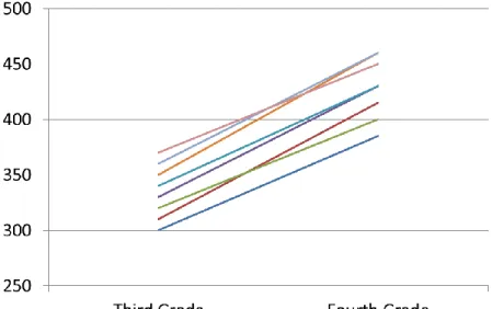
Figure 2-2. Example of students with very little difference in rates of change.
Figure 2-2 shows a class of students for which the individual growth rates change very little for each student from third grade to fourth grade. The correlation between the third and fourth grade tests is 0.91 and the correlation between the third grade test and the rate of change is 0.05.
Covariate Adjusted Model
Covariate Adjusted Models (CMs) model the current year’s test score as a function of prior test scores along with covariates. These included covariates are other classroom or student characteristics that are believed to impact student academic performance; the covariates “factor out” influence not attributable to the teacher (Lomax & Kuenzi, 2012). Some of the most common covariates used in education include socioeconomic status, ability to communicate in English (ELL status), and disability status. The CM below is a regression model
𝑦𝑖𝑡 = 𝜇𝑖𝑡+ 𝛽1𝑦𝑖,𝑡−1+ 𝑇𝑡+ 𝑒𝑡 (2 - 3) Where
𝜇𝑖𝑡 is the student specific mean for grade level at year t with adjustments for home and
school factors affecting student learning
𝛽1 is the vector of included covariates
𝑦𝑖,𝑡−1 is the score for the 𝑖𝑡ℎ student in the 𝑡 − 1𝑡ℎ year of data collection for 𝑡 ≥ 1
𝑇𝑡 is the teacher effect that estimates the impact the current teacher has on student
academic growth for year t
𝑒𝑖𝑡 is the residual error term for the 𝑖𝑡ℎ student in the 𝑡𝑡ℎ year of data collection that
represent the effects unique to student i due to chance that have not been controlled This model assumes that for each grade, teacher effect and the residual error terms (𝑒𝑖𝑡) are respectively i.i.d. normal random variable with mean zero, variance 𝜎Tt2 and 𝜎ϵt2, and independent of each other. Each year of data are fit separately allowing additional years of data be entered into the model as covariates (Daniel F McCaffrey et al., 2003).
The adjusted covariate model may be further subdivided into two analytic strategies: the random-effect strategy that produces more precise estimates at the cost of greater bias, or the fixed-effects strategy yielding less bias at the cost of precision (RTT TA Network Working, 2011). Models that specify teacher effects as “fixed-effects” assume the observed teachers are the only teachers of interest (Daniel F McCaffrey et al., 2003). This type of model yields measures that are solely dependent on individual teacher’s students thus possibly resulting in large deviation scores due to the variability in student scores (Daniel F McCaffrey et al., 2003). Caution should be taken when using fixed effects in models attached to high stakes
accountability. For teachers with small classes, the variability in student scores will likely result in a teacher effectiveness rating in one of the extremes of a distribution. However, Lomax and
Kunzi (2012) propose the fixed-effect model is preferred when an accountability system is in place.
Models that incorporate random-effects assume the observed teachers are a sample of a larger population of teachers of interest. When effects are treated as random, teacher effects are estimated from data from all teachers. Random effects cause “shrinkage” toward the mean. This shrinkage estimation is known as a Best Linear Unbiased Estimator (BLUE). While this
shrinkage reduces the variability in estimated teacher effects (Daniel F McCaffrey et al., 2003), it also forces teacher estimates to deviate away from the true unobserved effects. Unlike models incorporating fixed effects, the shrunken averages of random effects models minimizes the impact of the variation in student scores in small classes. A negative side to this is that truly ineffective teachers will receive higher scores than deserved and inversely, highly-effective teachers will receive lower scores than deserved.
Deciding on whether to use fixed or random effects in models depends on the VAM application in use, or inferences one wishes to derive. For instance, if variance components are of interest, random effects are preferred over fixed effects. While the R2 value in the fixed effects model can be used to make inference, fixed effects models do not provide direct estimates of variance among teachers as do random effects models (Daniel F McCaffrey et al., 2003). In general, if the possibility of underestimating the most and least effective teachers when estimates are shrunk toward the mean will not be detrimental to the inferences of interest, random effects are preferred. If the underestimation of most and least effective teachers is of concern for
inferential purposes, fixed effects are preferred (Daniel F McCaffrey et al., 2003). Essentially, if a school is to assume teachers are a random subset of all the teachers in the universe, the random effects model would be appropriate. However, if the teachers are thought to represent all teachers
in a relevant population, a fixed effect model would be appropriate (Goldschmidt, Choi & Beaudoin, 2012).
The CM is in wide use and championed to be easy to understand and to compute while controlling for effects of prior educational experiences (Mariano, McCaffrey, & Lockwood, 2010). Yet some statisticians caution their use to measure teacher effectiveness (Rowan et al., 2002) stating CMs do not sufficiently measure changes to student achievement (Rogosa, 1995; Stoolmiller & Bank, 1995). Johnson (n.d) and Tekwe et al. (2012) additionally showed this model to be relatively imprecise with the use of only two years of data and by fitting the model with each year separately, important information about prior years student performance which could account for individual student factors and help reduce bias is ignored (Daniel F McCaffrey et al., 2003).
Layered Model
The Layered Model (LM) links the impact of previous years’ teachers to latter years teachers (Daniel F McCaffrey, Lockwood, Koretz, & Louis, 2004; Sanders, 2006). The effects are thought to “layer” on top of one another. By linking current data to previous teachers, another layer of protection is afforded teachers against misclassification (Sanders, 2000). In the layered model, credit for student attainment will appropriately be assigned to a teacher as current scores effect the estimates of current and previous teachers (Sanders, 2000).
The LM can simultaneously model scores for multiple subjects through multiple years (RTT TA Network Working, 2011). The inclusion of covariates into LM are optional (RTT TA Network Working, 2011; Wiley, 2006). The LM measures teacher effects strictly as random effects with the inclusion of all teachers a priori considered “average” (a teacher effect of zero) until enough information is collected to prove otherwise (Sanders & Horn, 1994; Wright, White,