NBER WORKING PAPER SERIES
ASSET LOCATION IN TAX-DEFERRED AND CONVENTIONAL SAVINGS ACCOUNTS
John B. Shoven Clemens Sialm
Working Paper 7192 http://www.nber.org/papers/w7192
NATIONAL BUREAU OF ECONOMIC RESEARCH 1050 Massachusetts Avenue
Cambridge, MA 02138 June 1999
We would like to thank Ken Judd, Davide Lombardo, Jim Poterba, and Antonio Rangel for helpful comments on earlier drafts. All opinions expressed are those of the authors and not those of the National Bureau of Economic Research.
paragraphs, may be quoted without explicit permission provided that full credit, including © notic e, is given to the source.
Asset Location in Tax-Deferred and Conventional Savings Accounts John B. Shoven and Clemens Sialm NBER Working Paper No. 7192 June 1999
JEL No. G11,G23,H24
ABSTRACT
The optimal allocation of assets among different asset classes (such as stocks and bonds) has received considerable attention in financial theory and practice. On the other hand, investors have not been given much guidance about which assets should be located in tax-deferred retirement accounts and which in conventional savings accounts. This paper derives optimal asset allocations (which assets to hold) and asset locations (where to hold them) for a risk-averse investor saving for retirement. Locating assets optimally can significantly improve the risk-adjusted performance of retirement savings.
John B. Shoven Clemens Sialm
Department of Economics Department of Economics Stanford University Stanford University
Stanford, California 94305 Stanford, California 94305
and NBER sialm@leland.stanford.edu
Asset Location in Tax-Deferred and Conventional
Savings Accounts
by
John B. Shoven and Clemens Sialm
1
Introduction
One of the biggest financial challenges facing households is saving for retire-ment. Investors must decide how much to save, what to invest in, and which investments to hold in tax-deferred retirement accounts and which to hold in conventional taxable savings accounts. This paper addresses two of the main parts of the overall problem: which assets to hold and where to hold them. It does not deal with the choice of how much to save. The U.S. tax system influences the size and the composition of retirement savings by allowing in-dividuals to save in tax-qualified retirement vehicles (e.g., IRA, Roth-IRA, 401(k) accounts) and by exempting interest payments of certain assets (e.g., municipal bonds) from taxable income. This paper takes into account these institutional features and derives optimal portfolio choices for a risk-averse individual saving for retirement.
The optimal allocation between different asset classes such as stocks and bonds has received much attention in financial theory and practice since the seminal paper of Markowitz (1952). More recently several papers analyzed the effect of personal taxes on optimal asset allocation. Constantinides (1983) and Dammon and Spatt (1996) discuss optimal trading strategies if investors face personal taxes. Balcer and Judd (1987) examine the impact of capital income taxation on savings and the demand for corporate financial instru-ments under certainty. They show that the effective taxation depends on the investment horizon. Dybvig and Ross (1986) demonstrate that the taxation of asset returns can create clientele effects and derive the impact on asset pricing.
The aspect of this general topic which has been under-studied is the asset location choice—i.e. the choice of holding assets in tax-deferred retirement accounts or in conventional taxable savings accounts. Due to limitations on how much individuals can contribute to tax qualified accounts, households may want to or be forced to accumulate funds both inside a tax-deferred
account and outside such an account. This subject was introduced in Shoven and Sialm (1998) and Shoven (1999). This paper differs in two major respects from the previous two papers. First, the previous papers do not explicitly solve for the optimal portfolio choices (i.e., asset allocation and location); instead, they compare the simulated distributions of wealth levels at retire-ment for different heuristic portfolios. This paper solves for the choices which maximize expected utility. Second, Monte-Carlo simulations such as those in the previous papers do not give precise information about the extreme lower tails of the resulting wealth distributions. These outcomes have a large im-pact on expected utility if individuals are sufficiently risk-averse. This paper takes better account of the effects of those unlikely occurrences. Wang and Judd (1998) solve a dynamic savings allocation problem with tax-deferred and taxable accounts. This paper analyzes the asset location choice in much more depth and captures more completely important features of the U.S. tax code.
The actual behavior of individuals investing in tax-qualified accounts and taxable accounts is discussed by Bodie and Crane (1997) and Poterba and Samwick (1997). Poterba and Samwick analyze the relationship between age, birth cohorts, and portfolio structure for households using the Federal Re-serve Board’s Survey of Consumer Finances. They find that the composition of portfolios differ across birth cohorts. Bodie and Crane describe the as-set allocation behavior of participants of TIAA-CREF, an organization that manages self-directed retirement funds for the staff of some 6,000 universi-ties, secondary schools, and other nonprofit organizations. They examine the results of a survey that contains information on the composition of to-tal asset holdings—both inside and outside their tax-deferred accounts—of TIAA-CREF participants. They find that most households in the survey have significant amounts of money in both tax-deferred and in conventional accounts. The survey respondents locate a somewhat higher share of equity inside the tax-deferred account than outside. They tend to invest in taxable bonds and stocks in both environments. The respondents do not appear to take advantage of the potential benefits of optimal asset location.
There are three main results in this paper. First, the same asset located in different tax environments has a different mean after-tax return as well as a different variance. Returns of investments in tax-deferred accounts have generally a higher expectation and a higher standard deviation than returns on the same assets in conventional saving accounts. This implies that in-vestments in tax-deferred accounts are in general not perfect substitutes for
investments in conventional savings accounts even if the higher liquidity of taxable accounts is ignored. Second, the preferred asset location is deter-mined by the tax rates facing the returns, as well as the expectations and the standard deviations of the returns. The conventional wisdom is that it is wise to locate assets which face higher tax rates (such as taxable corpo-rate bonds) in a tax-qualified account while locating assets which are taxed less heavily (such as stocks or equity mutual funds) in conventional savings accounts. We show that this conventional wisdom is wrong under certain circumstances because stock returns have higher means and more risk than bond returns. Third, optimal asset location significantly improves the risk-adjusted performance of retirement saving. By simply adopting an optimal location strategy one can enhance the resources enjoyed in retirement by several percentage points.
The paper is organized as follows. Section 2 formulates the optimization problem of the investor. Section 3 derives the after-tax rates of return of different asset classes under the present U.S. tax system. Section 4 analyzes how asset characteristics and taxation influence the optimal asset location and allocation if investors can invest in stocks, taxable bonds, and tax-exempt municipal bonds. We discuss the effects of the taxation of nominal returns instead of real returns (i.e., inflation tax). The final section summarizes the major results of the paper.
2
The Model
This section presents the theoretical model used to derive optimal asset al-location and al-location choices. It is assumed that the investor maximizes expected utility at the time of retirement by choosing an optimal portfolio using tax-deferred and conventional savings accounts. The choice between consumption and saving is taken as exogenous.
To simplify the analysis, we examine the problem in a two-period model. The investor chooses her portfolio during her working career in the first pe-riod and withdraws the savings during retirement in the second pepe-riod. The investor has the choice to invest her saving of S inn risky assets which can be located either in a tax-deferred account (TDA) or a conventional savings account(CSA). The assets themselves are well-diversified portfolios of assets (they probably should be thought of as mutual funds of stocks or bonds). The investment horizon of the individual ishyears, which corresponds to the
length of the first period (i.e, the difference between retirement age and cur-rent age). Due to the limitations on how much individuals can contribute to a tax qualified account, they may want to accumulate funds in both locations. The maximum contribution to the TDA is C.
Assetiis assumed to have a nominal return ofri before taxes. The return before taxes will compound to Ri = (1 +ri)h−1 after h years. The return after taxes depends on the location and is denoted by RT DA
i orRCSAi . LettW
and tR denote the marginal income tax rates during the work career and at the time of retirement. If the investor saves $1 after taxes, she can contribute $1/(1−tW) to her TDA after taking into account the tax-deductibility of contributions to a tax-deferred account. This investment compounds at the before-tax rate of returnRi. The withdrawn benefits at the time of retirement are taxed at the future marginal income tax ratetR, which is assumed to be known in advance. The TDA-returns are identical to the before-tax returns if the tax rates do not change at the time of retirement (i.e, tW =tR). The after-tax return of asset i in a TDA after h years amounts to:
RT DAi = 1−tR
1−tW(1 +Ri)−1. (1)
Savings in a CSA are not deductible from taxable income and withdrawals are not taxed. Distributed returns (dividends, interest, and capital gains distributions) on assets held in a CSA are taxed annually. A fixed proportion of the average return ri of asset i is paid annually either as a short-run distributiondsr
i or as a long-run distributiondlri . The remainder 1−dsri −dlri
is the proportion of total returns that are accrued or unrealized capital gains. Short-run distributions are taxed at the full current marginal income tax rate tW and long-run distributions are taxed at the lower capital gains tax rate tC. The after-tax distributions are reinvested in the CSA. The total annual distributions simplify to di =dsr
i +dlri and the corresponding tax rate
simplifies to td
i = (tWdsri +tCdlri )/di. The savings compound after taxes at
the following rate:
riCSA=ri(1−di) + (1−tdi)diri =ri(1−tdidi). (2) The investor liquidates the CSA during retirement. She is required to pay capital gains taxes on the difference between the value of the portfolio and its cost basis. The cost basis per dollar of initial investment, Bi, is the sum of the initial dollar plus all the reinvested after-tax distributions. These re-investments grow geometrically at the rate rCSA
Bi = 1 + (1−tdi)diri 1 + (1 +rCSAi ) +. . .+ (1 +rCSAi )h−1 = 1 + (1−tdi)diri (1 +r CSA i )h−1 rCSA i ! (3) The after-tax return of asset iin a CSA after h years equals:
RiCSA= (1 +rCSAi )h−tC(1 +rCSAi )h−Bi−1. (4) We define the “effective tax rate” as the proportion of the total nominal asset returns collected by the government. The government would need to impose this effective tax on investment returns if it deferred the collection of the tax until the end of the time horizon h. τij = 1−Rji/Ri is the effective tax rate of asset i in the location j, where j = (CSA, T DA).1
τiT DA = tR−tW 1−tW (1 + 1/Ri), (5) τiCSA= 1− RCSA i Ri . (6) The initial savings S can be allocated to n assets in 2 locations. The corresponding weights are denoted by ωij. The investor is not allowed to short-sell assets. We assume for simplicity that the investor does not have any other sources of income during retirement.2 The nominal wealth level at retirement amounts to:
W =SX
i
X
j
ωij(1 +Rji). (7)
The price level at the time of retirement is P. The utility of final real wealth is given by a power-utility function with a constant coefficient of relative risk-aversion α. u(W) = ( 1 1−α(WP )1−α if α6= 1 ln(W P) if α= 1 (8) 1This definition of the effective tax rate is similar to Protopapadakis (1983).
2Other income sources might change the portfolio decisions of individuals. Introducing
relatively safe social security benefits would induce individuals to hold a smaller proportion of their portfolios in safe assets. Other risk sources such as health risk will also influence portfolio decisions. These extensions are not analyzed in this paper.
The investor maximizes the expected utility of real wealth at retirement subject to the short-selling constraints and the limitation of contributions to the TDA. max ω E(u( W P ))s.t. (9) X i X j ωji = 1 (10) ωij ≥0∀i, j (11) S 1−tW X i ωiT DA≤C (12) Asset i is said to have a preferred location in the TDA if its optimal proportion is higher in the TDA than in the CSA (i.e., ωT DA
i /
P
jωT DAj >
ωiCSA/
P
jωCSAj ) and a preferred location in the CSA if its optimal proportion
is higher in the CSA than in the TDA. The asset does not have a preferred location if its optimal proportion is identical in both taxable accounts or if the investor only contributes to one of the two accounts. Asset location is irrelevant in these two cases.
The optimization problem 9 cannot be solved analytically. Instead, we determine the optimal portfolio weights numerically assuming a log-normal distribution for the returns of the assets. The expected utility is computed using a multi-dimensional Gauss-Hermite quadrature with 10 nodes.3 The constrained optimization is performed using an active-set strategy.
3
Distribution of Returns
In this section we state the assumed distributions of asset returns and com-pute the after-tax returns of stocks, taxable bonds, and tax-exempt bonds in the two tax-environments.
3.1
Numerical Assumptions
Two major asset classes in financial markets are stocks and bonds. These two asset classes differ considerably in their characteristics and their rate of effec-tive taxation. Stocks have higher expected returns and a higher variability
of returns relative to bonds. Bonds usually pay most of their total returns as short-run distributions (interest payments) and only a small portion of their returns in the form of capital gains and losses.4 Income from bonds issued by state and local governments in the investor’s state of residence is completely exempt from federal and state income taxation. Because of this tax-exempt feature, the interest rate on these securities is below the rate on equally safe taxable bonds.5 Stocks pay a smaller portion of their total returns as short-run distributions (dividends and short-short-run capital gains). Capital gains and losses result from active trading by the investor or the mutual fund. Mutual funds differ considerably in their rate of asset turnover and in the proportion of their total annual returns distributed in the form of realized capital gains. Most mutual funds pay between 25 and 75 percent of their total annual re-turns as short- and long-run distributions. Individuals can influence the net distributions by trading their shares of mutual funds and thereby realizing accumulated capital gains and losses. Tax-efficient trading strategies result in lower and tax-inefficient strategies in higher annual distributions.6
The base case of the computations in section 4 assumes that the investor has a time horizon of 30 years. The coefficient of relative risk-aversion α is taken as 3, which can be characterized as moderate risk-aversion. The in-vestor can at most contribute half of her savings to the TDA.7 The marginal income tax rate is assumed to be identical during the working career and retirement in the base case. We analyze changes in marginal tax rates over the life-cycle. The base-case tax rates on short-run and long-run distribu-tions in the CSA are taken as 40 and 20 percent, roughly corresponding to the marginal federal income tax rate and capital gains tax rate faced by a high-income taxpayer. Some results are computed as well for
medium-4Zero-and low-coupon bonds are the exception.
5The implicit tax rate on municipal bonds is given byt
M = 1−rM/rB, whererM and rB denote the nominal returns of municipal bonds and corporate bonds. The difference between the yields on long-run municipal bonds and the yields on corresponding taxable bonds is surprisingly small. The implicit tax rate on long-run municipal bonds has been between 20 and 30 percent during the last 30 years; this is considerably lower than the maximum statutory marginal personal income tax rate (Shoven 1999).
6Constantinides (1983), Stiglitz (1983), and Dammon and Spatt (1996) argue that
opti-mal stock trading with personal taxes reduces the effective taxation considerably. Poterba (1987) and Auerbach, Burman, and Siegel (1998) find that avoidance of tax on realized capital gains is not prevalent and that the effective tax rate on realized capital gains is close to the statutory rate for a large proportion of investors.
7The contribution limit is thereforeC= S
income individuals (with tax rates of 30 and 20 percent) and for low-income individuals (with tax rates of 15 and 10 percent).
[Table 1 about here.]
Our assumptions regarding the distributions of real asset returns are shown in Table 1. The values correspond roughly to the historical record between 1926-1998 as summarized in Ibbotson (1999). The simple real re-turn of stock funds (S) has an expectation of 10 percent and a standard deviation of 25 percent. The corresponding moments are 4 and 8 percent for taxable bonds (B) and 2 and 6 percent for tax-exempt municipal bonds (M). The returns of the bonds assume an implicit tax rate of 28.6 percent for the municipal bonds, which is close to the average rate over the last thirty years.8 The real return of taxable bonds is set slightly higher than the current real yield on inflation-protected bonds to reflect a compensation for default and inflation risk. We perform sensitivity analyses on these assumptions to check the robustness of our results. The correlation coefficient is 0.25 be-tween stocks and taxable bonds, 0.2 bebe-tween stocks and tax-exempt bonds, and 0.95 between taxable and tax-exempt bonds. The rate of inflation has an average of 3 percent and a standard deviation of 4 percent. Inflation is negatively correlated with the real returns of all the assets.
We assume that the logarithms of the return relatives (i.e., one plus the simple returns) and the logarithm of the price level are jointly normally distributed. The moments of this distribution are derived using the moments of the simple returns shown in Table 1. The returns of the assets are assumed to be serially uncorrelated. The high serial correlation of inflation of 0.65 is taken into account when we compute the moments of price changes over long horizons.9
8Note that the implicit tax rate is defined for nominal returns. The assumptions from
Table 1 imply expected nominal returns of 7 and 5 percent for taxable and tax-exempt bonds, which corresponds to a 28.6 percent implicit tax rate on municipal bonds.
9A higher serial correlation increases the variance of inflation more than proportionally
if the time horizon exceeds 1 year. Letpj denote the logarithm of the price level at time j, where the initial price level is normalized to 1 (p0 = 0) and πj the logarithm of one plus the (simple) inflation rate iat timej. The price change during the time horizonh, ph=Phi=1πi, is normally distributed with a mean ofE(ph) =hE(π) and a variance of
V ar(ph) = h+2ρ(h(1−ρ)−(1−ρ h)) (1−ρ)2 V ar(π).
We assume in our base case that stock mutual funds distribute 50 percent of their total returns annually. The remaining 50 percent of the total returns are unrealized until the funds are withdrawn at the time of retirement. Short-run and long-Short-run annual distributions both equal 25 percent of the total returns. In the paper we often discuss the effect of different stock fund distributions. We define annual distributions as the fraction of the total returns which are distributed annually to the shareholders of the stock mutual funds and the fraction of those distributions which are taxed as short-run distributions. For example, funds with annual distributions of 75 percent are assumed to distribute 75 percent of their returns to the shareholders and 75 percent of those distributions are short-run capital gains. Actively managed funds with high asset turnover tend to distribute more than index funds and tax-efficient funds. Most funds distribute between 25 and 75 percent of their returns. The returns of both taxable and tax-exempt bonds are distributed completely as short-run income.
3.2
After-Tax Returns
The distribution of after-tax returns depends on the asset class and the tax-environment. Table 2 summarizes the means and the standard deviations of the after-tax annualized real returns of the three assets considered here for individuals in two different tax brackets. Distributions of total asset returns over long time periods are highly skewed to the right. To facilitate the interpretation of the returns we annualize the returns by taking the geometric mean of the long-run returns.10
[Table 2 about here.]
The real returns in the TDA equal the before-tax returns due to our base case assumption that marginal income tax rates do not change at the time of retirement. The net rate of return on assets in a TDA does not de-pend on the marginal income tax rate. Naturally, the average CSA returns are lower for high-income individuals than for medium-income individuals. 10The annualized moments of the geometric returns from Table 2 differ from the assumed
moments of the simple returns from Table 1. However, the underlying random distribution is the same. The means in Table 2 are defined as E (1 +Ri)1/h−1 and the variances as V ar (1 +Ri)1/h. The means in Table 1 are defined as E(ri) and the variances as V ar(ri).
Stocks have a higher average return and a higher standard deviation than bonds irrespective of the location. Savings in a TDA have a higher average return and a higher standard deviation than savings in a CSA for all assets except for tax-exempt municipal bonds. Municipal bonds have a higher ex-pected return than taxable bonds in the CSA for high- and medium-income individuals. However, the real after-tax return of taxable bonds is higher for low-income individuals. Returns in a CSA are less variable than the returns in a TDA because the tax system implicitly insures against losses in a CSA. Realized capital gains increase the tax liability and capital losses decrease the tax liability. This symmetric tax system dampens both gains and losses. The government does not insure against losses in a TDA at all. Assets in a TDA are taxed on a consumption tax basis, meaning that investors face the full (undampened) rates of return earned by the investments.11 The government does not insure against losses in a TDA at all. Assets in a TDA are taxed on a consumption tax basis, meaning that investors face the full (undampened) rates of return earned by the investments.
The effective taxation of taxable assets in a CSA is considerable. The government would need to impose this effective tax on nominal investment returns if it deferred the collection until at the end of the time horizon. Although the tax rates on short- and long-run distributions are assumed to be 40 and 20 percent for a high-income individual, the government will have taxed on average 62.6 percent of the nominal returns of bonds and 44.1 percent of the nominal returns of stocks after 30 years in the base case. Bonds face a higher effective tax because they pay all their returns as short-run distributions which are taxed at the marginal income tax rate, whereas stocks only distribute 50 percent of their returns annually and half of those distributions are taxed as long-run capital gains in the base case. Medium-11Our model does not capture two institutional facts. First, mutual funds are forced to
distribute realized capital gains to their shareholders but are prohibited from distributing losses. This fact might decrease the benefits of the implicit insurance in the CSA. Second, the tax code limits the deduction of realized capital losses from taxable income. If the capital losses are higher than the limit, then only the limit can be deducted from taxable income. However, it is possible to carry the remaining losses forward and to deduct them from future taxable income. Introducing those limitations does not change the major results of our paper significantly. To determine how important this limitation is we make the extreme assumption that capital losses can never be deducted from taxable income. This decreases the mean real return of stocks in the CSA from 5.43 to 5.42 percent and increases the standard deviation from 3.74 to 3.76 percent for a high-income individual and does only change the returns of bonds marginally.
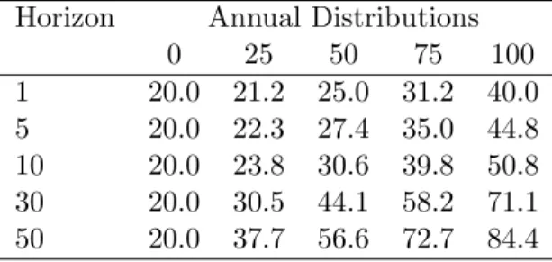
income individuals (tW = 0.3 and tC = 0.2) pay effectively on average 51.1 percent taxes on bonds and 39.4 percent on stocks. Low-income individuals (tW = 0.15 and tC = 0.1) are still taxed on average 29.2 and 21.7 percent on the two assets. The effective tax rates increase both with the time horizon and the level of annual distributions as shown in Table 3 for high-income individuals. Investing in assets with annual distributions of 25 instead of 75 percent results in 66.4 percent more wealth with a 30 year horizon.
[Table 3 about here.]
4
Optimal Portfolio Choice
In this section we analyze how asset characteristics and taxation influence optimal asset allocation and location. First, we derive numerically the opti-mal portfolio for an investor who chooses between a bond and a stock mutual fund. Second, we add tax-exempt municipal bonds as a feasible investment choice. Third, we show that asset location is also important for risk-tolerant investors who only invest in stock mutual funds.
4.1
Choice of Stocks and Taxable Bonds
When choosing between a corporate bond fund and a particular equity mu-tual fund, optimal asset location depends primarily on the proportion of returns that the equity fund distributes annually as dividends and capital gains (tax effect). Funds with high annual (potentially taxable) distributions should be located in a TDA. We show that return effects (i.e., the effective tax increases with the return of an asset) and risk effects (i.e., investments in a TDA are more risky than investments in a CSA) are secondary effects which under certain circumstances can outweigh the primary tax effect. As-set location influences the performance of a portfolio substantially.
A high-income individual should take full advantage of tax-deferred sav-ings and contribute the limit to the TDA. She should invest 6.5 percent of her assets in equities in the TDA, 43.5 percent in bonds in the TDA, and the remaining 50 percent in stocks in the CSA in the base case. Bonds have a preferred location in the TDA and stocks in the CSA if stocks distribute 50 percent of their returns annually. The location preference of stocks shifts to the TDA if stocks distribute more than 92 percent of their returns as shown
in Figure 1. This result contradicts conventional wisdom which advises to put the asset with the higher tax rate in the TDA. Although bonds face higher tax rates than stocks, stocks have higher expected returns and gain more by compounding without deductions of taxes in the TDA. If the an-nual distributions of the equity fund are below 17 percent then the investor should not hold stocks in the TDA at all. The investor increases the share of stocks in the TDA as the annual distribution of stock funds increases. This portfolio shift towards stocks compensates for the higher effective taxation facing stocks in the CSA at higher distribution levels.
[Figure 1 about here.]
The asset allocations and locations do not differ much for medium- and low-income individuals. Individuals facing lower tax rates hold fewer stocks in the TDA in the base case (4.9 and 0.0 percent for the medium- and low-income individuals). The location preference of stocks shifts to the TDA if stocks distribute more than 89 percent for medium-income individuals and 87 percent for low-income individuals. The portfolio choice is not affected significantly for individuals expecting a lower or higher marginal income tax rate during retirement.
To determine whether asset location is economically significant we com-pare the gains from asset location to the gains from the existence of a tax-deferred account. We compute the expected utility of an investor in three different environments. In a first environment investments can only be made in a taxable CSA (NTDA). A second environment allows investments in a TDA but restricts investors to hold the same relative proportions in the CSA and the TDA (NL). A third environment allows investments in a TDA and does not restrict the asset location. This third environment corresponds to the optimization problem described in section 2. For a better comparison of the three environments we compute the certainty equivalents of the expected utilities. It is defined as:
ce(E(u)) =u−1(E(u)) =
(
((1−α)E(u))1−1α if α6= 1
exp(E(u)) if α= 1 (13)
Let ce denote the certainty equivalent in the unrestricted environment. The certainty equivalents in the environment without a TDA and without asset location are denoted byceN T DAandceN L. The gain due to the existence
of a TDA is ceN L/ceN T DA−1 and the gain due to optimal asset location is
ce/ceN L−1.
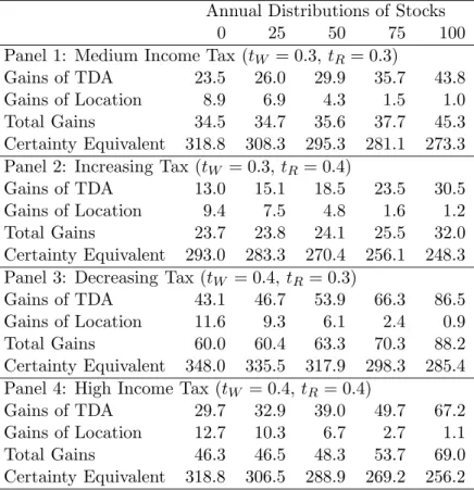
Table 4 summarizes the certainty equivalents in the unrestricted model and the gains from asset location between the three environments. Panel 4 shows the values for a high-income individual facing the same tax rates during the working career and during retirement. The certainty equivalent in the unrestricted environment equals 288.9 percent of the initial savingSfor this high-income individual in the base case with an equity fund distributing 50 percent of its total return. Choosing stock portfolios with lower annual distributions increases the wealth at retirement considerably. The certainty equivalent increases by 13.9 percent if the the high-income individuals shifts from a mutual fund with 75 percent distribution (typical for an actively managed fund) to a fund with 25 percent distribution (typical for a tax-efficient fund). The availability of a TDA corresponds to an increase in the certainty equivalent of retirement wealth of 39.0 percent in the base case. The benefits of a TDA increase with the annual distributions of the stocks. Asset location improves the performance of a portfolio significantly. Optimal asset location adds 6.7 percent to the benefits of a TDA in the base case. The gains of asset location are particularly high if the available assets differ considerably in their characteristics, that is if stocks differ from bonds by distributing considerably less than 100 percent. The benefits of asset location are computed relative to a symmetric asset location. Other sub-optimal asset locations can reduce retirement wealth considerably more.
[Table 4 about here.]
Panel 1 of Table 4 shows that a medium-income individual has a slightly higher certainty equivalent than the high-income individual. The gains of a TDA and asset location are slightly lower because the tax-deferral is less valuable if investors face lower taxes. Saving in tax-deferred accounts is particularly beneficial if tax rates are expected to be lower during retire-ment than during the working career as shown in Panel 3. Individuals can deduct their contributions from their taxable income when they face higher tax rates and they pay the taxes on the withdrawn benefits when their taxes are lower. Panel 2 shows that contributions to the TDA are beneficial even if the marginal income tax rates are expected to rise from 30 to 40 percent at retirement.
The following computations check the robustness of our results by chang-ing the assumptions about risk-aversion, expected returns, and standard
deviations. Figure 2 shows the portfolio composition at different levels of risk-aversion. Contributions to the TDA equal the contribution limit for plausible levels of risk-aversion. Investors invest exclusively in stock funds if their risk-aversion is lower than α = 1.4. As their risk-aversion increases they shift towards bonds. The preferred location of stocks remains the CSA.
[Figure 2 about here.]
The preferred location of bonds does not depend on the level of expected returns and the standard deviation of stocks for high-income individuals as shown in Figures 3 and 4. Investors shift their portfolios towards stocks as their expected return and their risk decreases.
[Figure 3 about here.] [Figure 4 about here.]
4.2
Choice of Stocks, Taxable and Tax-Exempt Bonds
This section adds tax-exempt municipal bonds to the asset choices. The plied tax rate on municipal bonds is assumed to equal 28.6 percent. This im-plied tax is smaller than the marginal income tax rate of high- and medium-income individuals, which determines the taxes paid on interest payments of taxable bonds. The computations assume that tax-exempt and taxable bonds are highly but not perfectly correlated. We show that municipal bonds should be located in the CSA and corporate bonds in the TDA. Stocks have a preferred location in the TDA if their distributions are sufficiently high.
A high-income individual should invest 6.5 percent in stocks in the TDA, 43.5 percent in bonds in the TDA, and the remaining 50 percent in stocks in the CSA if stocks distribute 50 percent of their total returns annually. The investor chooses exactly the same portfolio as without municipal bonds. Figure 5 shows that municipal bonds are only held if the stocks distribute more than 52 percent annually. Municipal bonds have a preferred location in the CSA and taxable bonds in the TDA. The preferred location of stocks shifts from the CSA to the TDA if they are sufficiently tax-inefficient. A medium-income individual holds the same portfolio as in an environment without municipal bonds if stocks distribute 50 percent. The substitution of municipal bonds in the CSA for taxable bonds in the TDA occurs at a slightly higher level of annual distributions of the stocks for medium-income
than for high-income individuals. Low-income individuals never invest in tax-deferred municipal bonds and choose the same portfolios as in an en-vironment without them. Investment practitioners suggest that individuals hold municipal bonds if their marginal tax rate on ordinary income is higher than the implicit tax rate of municipal bonds. This advice is not always correct for individuals saving in both tax environments. The relevant com-parison in our case is the implied tax on municipal bonds relative to the tax on stocks in the CSA. Individuals should put bonds in the TDA and mostly stocks in the CSA if the taxes on stocks are lower than the implied taxes on municipal bonds. This reduces the demand of investors for municipal bonds and might explain the low implicit tax rate on them which is often perceived to be puzzling.12
[Figure 5 about here.]
Adding tax-exempt bonds does only affect the certainty equivalent if stock funds are sufficiently inefficient. Otherwise investors do not hold tax-exempt bonds and their portfolios are identical to an environment without tax-exempt bonds. The introduction of tax-exempt bonds increases the cer-tainty equivalent of high-income individuals from 269.2 to 285.1 if stocks distribute 75 percent of their returns annually. The gains of a TDA are 29.1 percent and the gains of optimal location are 8.8 percent in this case.
4.3
Choice of Two Stocks
In this section we consider the case of allocating assets between two stock mutual funds. In sections 4.1 and 4.2 we showed that investors with low risk-aversion should invest exclusively in stocks. Asset location is important in this case if investors have the choice between stock funds with different characteristics. The two stock funds might differ in the market capitalization of the stocks held (small vs. large caps), in their nationality (domestic vs. foreign stocks), or they might be constructed to take full advantage of the different tax environments (e.g., with one portfolio including mostly assets with highly taxed short-run distributions and the other portfolio including assets with lightly taxed long-run capital gains). We show that the opti-mal asset location depends primarily on the proportion of returns that are 12This explanation of the low implicit tax rate on municipal bonds is similar to Mankiw
distributed annually as dividends and capital gains. Assets with high an-nual (potentially taxable) distributions should be located in a TDA. Asset location can influence the performance of a portfolio substantially.
Consider a high-income investor with a risk aversion of α = 1. This investor should not hold taxable nor tax-exempt bonds. The investor can choose between two stock mutual funds. The mutual funds are assumed to have the same expected return of 10 percent and the same standard deviation of 25 percent. The correlation between their returns amounts to 0.5. The other assumptions are given in section 3. In Figure 6 we change the annual distributions of stock fund 1 and keep the total distributions of stock fund 2 constant at 50 percent. If both assets distribute 50 percent of total returns, then it is optimal to invest the initial savings equally in the four possible choices.13 That is, the TDA should be used to the maximum extent possible and both environments would hold the same proportions of stock fund2 1 and 2. If stock fund 1 distributes more (less) than 50 percent then its preferred location is in the TDA (CSA).
[Figure 6 about here.]
The availability of a TDA increases the certainty equivalent by 17.1 per-cent if both stocks distribute 50 perper-cent of their returns annually. The gains of asset location are zero in this case because the optimal asset location corre-sponds exactly to the symmetric asset location (i.e., the proportions of stock 1 in the TDA and the CSA are identical). The gains from asset location increase with more asymmetric asset characteristics. An optimal asset loca-tion generates an increase in the certainty equivalent of 4.1 percent relative to the symmetric asset allocation if stock fund 1 distributes 25 percent of its returns and fund 2 distributes 75 percent of its returns. Asset location is therefore as well relevant for risk-tolerant individuals investing in just one asset class.
5
Conclusions
This paper derives optimal asset locations and allocations for risk-averse in-vestors saving for retirement. It confirms the desirability of accumulating as-sets in tax-deferred accounts and suggests that certain asas-sets are best suited 13This symmetric allocation is strictly better than any other allocation because it
to taxable and tax-deferred accounts. The most important determinant of asset location is the proportion of returns distributed annually as income and capital gains. We show that expected returns and standard deviations of as-sets may as well influence the asset location choice. The paper shows that coupon bonds and stocks with high annual distributions have a preferred lo-cation in the tax-deferred environment and that tax-exempt municipal bonds and stocks with low annual distributions have a preferred location in conven-tional savings accounts. One of the key findings of this paper is that asset location choice can affect welfare in retirement by significant amounts. Asset location matters both for high-income and low-income individuals and for risk-tolerant and risk-averse investors.
References
Auerbach, A. J., L. E. Burman, and J. M. Siegel (1998). Capital gains taxation and tax avoidance: New evidence from panel data. NBER Working Paper 6399, NBER.
Balcer, Y. and K. L. Judd (1987). Effects of capital gains taxation on life-cycle investment and portfolio management.Journal of Finance 42(3), 743–758.
Bodie, Z. and D. B. Crane (1997, November). Personal investing: Advice, theory, and evidence. Financial Analysts Journal, 13–23.
Constantinides, G. (1983). Capital market equilibrium with personal tax. Econometrica 51(3), 611–636.
Dammon, R. M. and C. S. Spatt (1996). The optimal trading and pricing of securities with asymmetric capital gains taxes and transaction costs. Review of Financial Studies 9(3), 921–952.
Dybvig, P. H. and S. A. Ross (1986). Tax clienteles and asset pricing. Journal of Finance 41(3), 751–762.
Ibbotson (1999). Stocks, Bonds, Bills, and Inflation: 1999 Yearbook. Chicago: Ibbotson Associates.
Judd, K. L. (1998).Numerical Methods in Economics. Cambridge: MIT. Mankiw, N. G. and J. M. Poterba (1996). Stock market yields and the
pricing of municipal bonds. NBER Working Paper 5607, NBER. Markowitz, H. M. (1952). Portfolio selection. Journal of Finance 7(1),
77–91.
Poterba, J. M. (1987). How burdensome are capital gains taxes? Evidence from the United States. Journal of Public Economics 33, 157–172. Poterba, J. M. and A. A. Samwick (1997). Household portfolio allocation
over the life cycle. NBER Working Paper 6185, NBER.
Protopapadakis, A. (1983). Some indirect evidence on effective capital gains tax rates. Journal of Business 56(2), 127–138.
Shoven, J. B. (1999). The location and allocation of assets in pension and conventional savings accounts. NBER Working Paper 7007, NBER. Shoven, J. B. and C. Sialm (1998). Long run asset allocation for retirement
Stiglitz, J. E. (1983). Some aspects of the taxation of capital gains.Journal of Public Economics 21, 257–294.
Wang, S.-P. and K. L. Judd (1998). Solving a savings allocation problem by numerical dynamic programming with shape-preserving interpolation. Stanford University, mimeo.
List of Figures
1 Portfolio Composition . . . 21
2 Changes in Risk Aversion . . . 22
3 Changes in the Expected Return of Stocks . . . 23
4 Changes in the Risk of Stocks . . . 24
5 Portfolio Choice with Tax-Exempt Bonds . . . 25
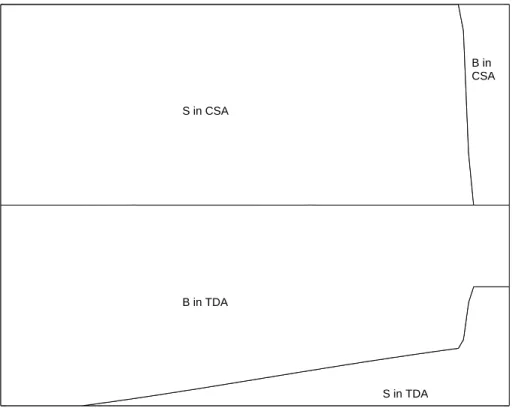
Figure 1: Portfolio Composition
The cumulative portfolio composition is depicted for a high-income individual at different levels of annual distributions of the stock fund. The investor should invest 6.5 percent in stocks in the TDA, 43.5 percent in bonds in the TDA, and 50 percent in stocks in the CSA if stocks distribute 50 percent of their returns annually. Stocks have a preferred location in the CSA if they distribute less than 92 percent of their annual returns.
0 0.1 0.2 0.3 0.4 0.5 0.6 0.7 0.8 0.9 1 0 0.1 0.2 0.3 0.4 0.5 0.6 0.7 0.8 0.9 1
Annual Distributions of Stocks
Weights S in TDA B in TDA S in CSA B in CSA
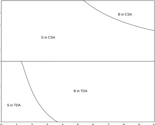
Figure 2: Changes in Risk Aversion
The proportion invested in stocks decreases as the risk-aversion increases. Stocks have a preferred location in the CSA. Stocks are assumed to distribute 50 percent of their returns.
0 1 2 3 4 5 6 7 8 9 10 0 0.1 0.2 0.3 0.4 0.5 0.6 0.7 0.8 0.9 1 Risk Aversion Weights S in TDA B in TDA S in CSA B in CSA
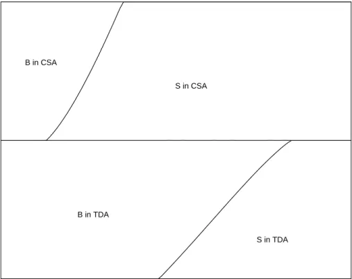
Figure 3: Changes in the Expected Return of Stocks
The proportion invested in stocks increases as their return increases. Bonds have a preferred location in the TDA. Stocks are assumed to distribute 50 percent of their returns.
0 0.02 0.04 0.06 0.08 0.1 0.12 0.14 0.16 0.18 0.2 0 0.1 0.2 0.3 0.4 0.5 0.6 0.7 0.8 0.9 1
Expected Return of Stocks
Weights
S in TDA B in TDA
S in CSA B in CSA
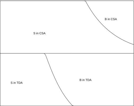
Figure 4: Changes in the Risk of Stocks
The proportion invested in stocks decreases as their standard deviation de-creases. Bonds have a preferred location in the TDA. Stocks are assumed to distribute 50 percent of their returns.
0 0.05 0.1 0.15 0.2 0.25 0.3 0.35 0.4 0.45 0.5 0 0.1 0.2 0.3 0.4 0.5 0.6 0.7 0.8 0.9 1
Standard Deviation of Stocks
Weights
S in TDA
B in TDA S in CSA
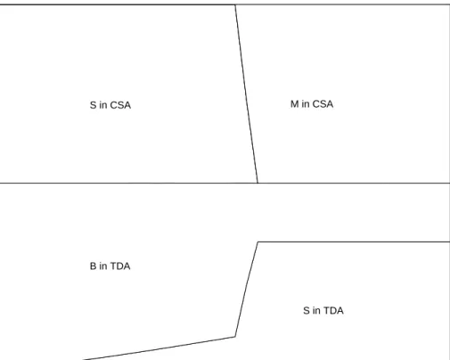
Figure 5: Portfolio Choice with Tax-Exempt Bonds
A high-income individual holds exactly the same portfolio as in the environ-ment without tax-exempt bonds if stocks distribute 50 percent of their total returns annually. Municipal bonds in the CSA replace taxable bonds in the TDA if the stock funds distribute more than 52 percent annually.
0 0.1 0.2 0.3 0.4 0.5 0.6 0.7 0.8 0.9 1 0 0.1 0.2 0.3 0.4 0.5 0.6 0.7 0.8 0.9 1
Annual Distributions of Stocks
Weights
S in TDA B in TDA
M in CSA S in CSA
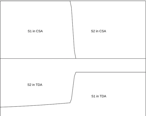
Figure 6: Two Stock Funds
The cumulative portfolio composition is depicted for a high-income individual investing in two stocks which differ only in their annual distributions. Stock fund 2 is assumed to distribute 50 percent of its returns annually. The investor should invest equal proportions in the four choices if both stock funds distribute 50 percent of their returns. The fund with the higher distributions has a preferred location in the TDA.
0 0.1 0.2 0.3 0.4 0.5 0.6 0.7 0.8 0.9 1 0 0.1 0.2 0.3 0.4 0.5 0.6 0.7 0.8 0.9 1
Annual Distributions of Stock Fund 1
Weights
S1 in TDA S2 in TDA
S2 in CSA S1 in CSA
List of Tables
1 Assumptions of Returns . . . 28
2 After-Tax Returns . . . 29
3 Effective Tax Rates on Stocks in a CSA . . . 30
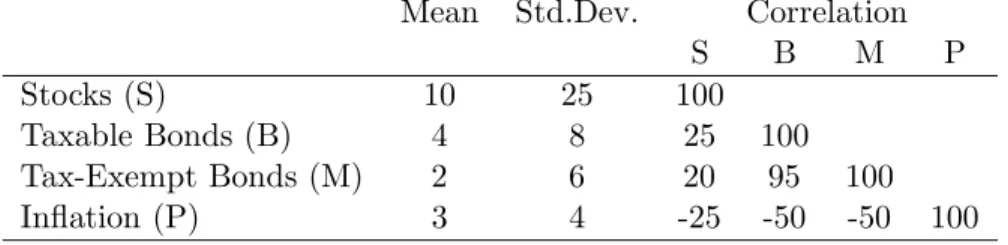
Table 1: Assumptions of Returns
The table lists the means, standard deviations, and correlations of the simple real asset returns and of the rate of inflation. All values are in percent.
Mean Std.Dev. Correlation
S B M P
Stocks (S) 10 25 100
Taxable Bonds (B) 4 8 25 100 Tax-Exempt Bonds (M) 2 6 20 95 100
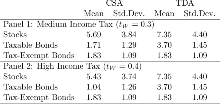
Table 2: After-Tax Returns
The table lists the distribution of the annualized geometric real returns of investments in a CSA and a TDA for individuals in two different tax brackets. The investment horizon equals 30 years. All values are in percent.
CSA TDA
Mean Std.Dev. Mean Std.Dev. Panel 1: Medium Income Tax (tW = 0.3)
Stocks 5.69 3.84 7.35 4.40
Taxable Bonds 1.71 1.29 3.70 1.45 Tax-Exempt Bonds 1.83 1.09 1.83 1.09 Panel 2: High Income Tax (tW = 0.4)
Stocks 5.43 3.74 7.35 4.40
Taxable Bonds 1.04 1.26 3.70 1.45 Tax-Exempt Bonds 1.83 1.09 1.83 1.09
Table 3: Effective Tax Rates on Stocks in a CSA
The table reports the average effective tax rates of stock mutual funds held in a CSA for a high-income individual at different time horizons and annual distributions. All values are in percent.
Horizon Annual Distributions
0 25 50 75 100 1 20.0 21.2 25.0 31.2 40.0 5 20.0 22.3 27.4 35.0 44.8 10 20.0 23.8 30.6 39.8 50.8 30 20.0 30.5 44.1 58.2 71.1 50 20.0 37.7 56.6 72.7 84.4
Table 4: Gains With Stocks and Taxable Bonds
The table lists the percentage changes in the certainty equivalents of different investment environments if the individual can invest in stocks and taxable bonds. ‘Gains of TDA’ denote the gains which result from the availability of a TDA if the investor locates the asset classes symmetrically in the CSA and the TDA. ‘Gains of Location’ are the additional gains from locating the assets optimally between the CSA and the TDA. The products of those two gains are the ‘Total Gains’. The ‘Certainty Equivalent’ is for an environment with a TDA and optimal asset location. It is expressed in percent of the initial savings.
Annual Distributions of Stocks
0 25 50 75 100
Panel 1: Medium Income Tax (tW = 0.3,tR= 0.3)
Gains of TDA 23.5 26.0 29.9 35.7 43.8 Gains of Location 8.9 6.9 4.3 1.5 1.0 Total Gains 34.5 34.7 35.6 37.7 45.3 Certainty Equivalent 318.8 308.3 295.3 281.1 273.3 Panel 2: Increasing Tax (tW = 0.3,tR= 0.4)
Gains of TDA 13.0 15.1 18.5 23.5 30.5 Gains of Location 9.4 7.5 4.8 1.6 1.2 Total Gains 23.7 23.8 24.1 25.5 32.0 Certainty Equivalent 293.0 283.3 270.4 256.1 248.3 Panel 3: Decreasing Tax (tW = 0.4,tR= 0.3)
Gains of TDA 43.1 46.7 53.9 66.3 86.5 Gains of Location 11.6 9.3 6.1 2.4 0.9 Total Gains 60.0 60.4 63.3 70.3 88.2 Certainty Equivalent 348.0 335.5 317.9 298.3 285.4 Panel 4: High Income Tax (tW = 0.4,tR= 0.4)
Gains of TDA 29.7 32.9 39.0 49.7 67.2 Gains of Location 12.7 10.3 6.7 2.7 1.1 Total Gains 46.3 46.5 48.3 53.7 69.0 Certainty Equivalent 318.8 306.5 288.9 269.2 256.2