Copyright belongs to the author. Small sections of the text, not exceeding three paragraphs, can be used
provided proper acknowledgement is given.
The
Rimini Centre for Economic Analysis
(RCEA) was established in March 2007. RCEA is a private,
nonprofit organization dedicated to independent research in Applied and Theoretical Economics and related
fields. RCEA organizes seminars and workshops, sponsors a general interest journal
The Review of
Economic Analysis
,
and organizes a biennial conference:
The Rimini Conference in Economics and Finance
(RCEF)
. The RCEA has a Canadian branch:
The Rimini Centre for Economic Analysis in Canada
(RCEA-Canada). Scientific work contributed by the RCEA Scholars is published in the RCEA Working Papers and
Professional Report series
.
The views expressed in this paper are those of the authors. No responsibility for them should be attributed to
the Rimini Centre for Economic Analysis
.
The Rimini Centre for Economic Analysis
Legal address: Via Angherà, 22 – Head office: Via Patara, 3 - 47900 Rimini (RN) – Italy
[email protected]
WP 11-19
Paolo Zagaglia
University of Bologna
The Rimini Centre for Economic Analysis (RCEA)
F
ORECASTING
L
ONG
-T
ERM
I
NTEREST
R
ATES WITH A
D
YNAMIC
G
ENERAL
E
QUILIBRIUM
M
ODEL OF THE
E
URO
A
REA
:
Forecasting long-term interest rates with a
dynamic general equilibrium model of the Euro area:
The role of the feedback
Paolo Zagaglia
∗This version: March 28, 2011
Abstract
This paper studies the forecasting performance of the general equilibrium model of bond yields of Marzo, Söderström and Zagaglia (2008), where long-term interest rates are an integral part of the monetary transmission mechanism. The model is estimated with Bayesian methods on Euro area data. I compare the out-of-sample predictive performance of the model against a variety of competing specifications, including that of De Graeve, Emiris and Wouters (2009). Forecast accuracy is evaluated through both univariate and multivariate measures. I also control the statistical significance of the forecast differences using the tests of Diebold and Mariano (1995), Hansen (2005) and White (1980). I show that taking into account the impact of the term structure of interest rates on the macroeconomy generates superior out-of-sample forecasts for both real variables, such as output, and inflation, and for bond yields.
Keywords: Yield curve, general equilibrium models, Bayesian estimation, forecasting.
JEL Classification: E43, E44, E52.
∗Department of Economics, University of Bologna. E-mail: [email protected]. This paper was written while
I was visiting the Monetary Policy Strategy Division of the European Central Bank and the Research Unit of the Bank of Finland. I am grateful to both institutions for their kind hospitality. Massimiliano Marzo, Massimo Rostagno and Ulf Söderström encouraged me to pursue this project, and provided countless suggestions. I have benefitted from comments on an earlier version from seminar participants at the ECB, the Bank of Finland and Sveriges Riksbank. In particular I thank Gianni Amisano, Luca Benati, Efrem Castelnuovo, Juha Kilponen, Stefano Nardelli, Jouko Vilmunen and Mattias Villani. This research was carried out by the author for purely academic purposes and without financial support from any private or public institution.
1
Introduction
Different frameworks have been proposed to study the relation between movements in the term structure of interest rates and business cycle fluctuations.1 The so-called ‘macro-finance’ models describe the evolution of macroeconomic variables, such as output and inflation, from reduced-form aggregate demand and Phillips curves (e.g., see Rudebusch and Wu, 2003 and Hördahl, Tristani, and Vestin, 2006). One of the shortcomings of this approach is that bond yields at different maturities are priced from ‘ad hoc’ stochastic discount factors that do not arise from microfounded problems of intertemporal utility maximization.
Various papers have tried to fill in this gap in the literature by modelling the macroeconomy through dynamic stochastic general equilibrium models (DSGE). In this way, bond yields can be priced by using kernels that are consistent with the utility function of a representative consumer. The modelling approaches of De Graeve, Emiris and Wouters (2009), Doh (2008) and Amisano and Tristani (2008) represent only a few examples. De Graeve, Emiris and Wouters (2009) augment the loglinearized model of Smets and Wouters (2003) with model-consistent yields for longer maturities. They estimate their model on U.S. data with Bayesian methods and introduce measurement errors in the yields to mimic term premia. Doh (2008) and Amisano and Tristani (2008) capture the variability of risk premia in the U.S. by estimating the second-order Taylor approximation of a small New-Keynesian model with time-varying volatilities of the structural shocks.
The available contributions focus on generating a realistic variability in term premia that allows to match the observed changes in bond yields. However, they disregard the role that changes in the term structure of interest rates play for macroeconomic fluctuations. These models price the term structure by using the kernel for one period bonds. Since the kernel is extracted from the solution of the model economy, this pricing strategy ignores the issue of the ‘feedback’ from bond yields to the macroeconomy. While the these models imply effects of monetary policy and the macroeconomy on the term structure, they do not feature effects in the opposite direction, from the term structure (and term premia) to the macroeconomy and monetary policy. This is a strong assumption that casts a shadow on the ability of these models to provide understanding on the interaction between bond yields and the macroeconomy.
The relevance of changes in asset prices for the monetary transmission mechanism is often stressed by prominent policymarkers. For instance, on April 28, 2009, during a keynote lecture at the International Center for Monetary and Banking Studies, Lorenzo Bini Smaghi, Member of the Executive Board of the European Central Bank, has reviewed the arguments for quantitative easing, suggesting that
“When long-term government bonds are purchased, the yields on privately issued securities are expected to decline in parallel with those on government bonds. (...) If long-term interest rates were to fall, this would stimulate longer-term investments and hence aggregate demand, thereby supporting price stability.”
The role of the term structure for macroeconomic fluctuations was remarked also by Jean-Claude Trichet, president of the European Central Bank, during a Testimony before the Committee on Economic and Monetary Affairs of the European Parliament on September 14, 2005:
1Extensive surveys are provided in Diebold, Piazzesi, and Rudebusch (2005) for the literature on affine term structure
“(...) investment should benefit from the exceptionally low level of both nominal and real market interest rates prevailing across the entire maturity spectrum.”
This is indicative of the conventional wisdom that, by affecting the term structure, a central bank can control part of the monetary transmission mechanism. On top of the informal accounts, Diebold, Rudebusch, and Aruoba (2006) and Marzo, Söderström and Zagaglia (2008) provide empirical evidence from block exogeneity tests which suggests that the feedback from the term structure is statistically significant in vector autoregressive models.
Despite the lack of feedback, the DSGE models of the term structure described earlier have been used for forecasting both government bond yields, and output and inflation. Failing to account for the feedback from bond yields can be a source of misspecification that affects the predictive ability of the model. In this paper, I investigate whether accounting for the role of the term structure in the monetary transmission mechanism delivers gains of predictive performance. I study the forecast ability of the model of Marzo, Söderström and Zagaglia (2008) and compare it with that of models that lack the feedback from the term structure.
The framework of Marzo, Söderström and Zagaglia (2008) builds on the portfolio approach of Tobin (1969, 1982) to introduce segmentation in financial markets. Due to frictions that make changes in bond holdings costly to households, the model generates positive holdings of different types of bonds in equilibrium. In this paper, I use a version of the model with short, medium and long-term bonds. I assume that changing the ratios between the bond and money holdings generates a real cost for the household. The maturity profile of bonds is then determined by the propensity of households to reallocate resources between each bond and money. This mechanism creates a link between monetary aggregates and bond prices, and allows to study the role of money demand shocks when bond prices matter for the macroeconomy.
The model presents two channels of monetary transmission between the term structure and the real variables. Since long-term bonds are part of households’ wealth, they determine the shadow value of the budget constraint and affect consumption choices. This is a standard wealth channel. When agents have a desire to hold a certain ratio between bonds of longer maturities and money, long-term rates generate changes in money demand. This is a money demand channel. By assuming that money provides liquidity services for the purchase of consumption goods, I strengthen the link between bond prices and consumption through money demand. Moreover, following Andrés, López-Salido and Vallés (2006), I introduce a money target target in the central bank’s monetary policy rule. Since short-term interest rates respond to fluctuations of money demand around its long-run value, changes in long-term interest rates feed through to output via the pricing of short-term bonds.
I use Bayesian techniques to estimate the general equilibrium model of bond yields of Marzo, Söderström and Zagaglia (2008) on quarterly Euro area data for the period 1980:1 to 2007:2. Following Adolfson, Lindé and Villani (2007), I evaluate the out-of-sample rolling forecasts of the model using both univariate and multivariate accuracy criteria. I also compute the tests for predictive ability of Diebold and Mariano (1995) and the reality check tests of White (1980), and the test for superior predictive ability of Hansen (2005).
In order to understand what feedback channels from the term structure are important for capturing the properties of the data, I compare the out-of-sample predictive performance of the benchmark DSGE model with those of alternative model versions.To get a flavor of how important the money demand channel is for the feedback, I estimate a model variant with strongly-separable utility between
consumption and money, and without money target in the monetary policy rule. The question remains about how well the model of the term structure helps to understand changes in output and inflation. After removing the bond market frictions, I obtain a New Keynesian model with non-separability between consumption and money balances. The bond and money market frictions that generate endogenous long-term yields imply restrictions that are different from those of the expectations hypothesis of the term structure. Hence, an appropriate competing model for the term structure is that of De Graeve, Emiris and Wouters (2009).
The results suggest that removing the money demand channel for feedback worsens the predictive performance of the model both for the term structure yields and for money. The model with the endogenous term structure predicts output and inflation better than a model version without the term structure. This indicates that the modelling strategy for the term structure pursued in the benchmark DSGE conveys relevant information for the monetary transmission mechanism. Finally, the forecast comparison with the model of De Graeve, Emiris and Wouters (2009) accounting for the feedback through the financial market frictions presented here improves substantially the predictive performance for bond prices.
The paper is organized as follows. Section 2 presents the DSGE model of the term structure. The properties of the dataset are described in Section 3. Section 4 discusses the deterministic steady state, the calibrated parameters and the prior assumptions for the Bayesian estimation. In Section 5 I present the competing restricted (DSGE) and unrestricted (VAR and BVAR) models. In Section 6 I outline the forecast accuracy criteria. The results from both the Bayesian estimation and the out-of-sample forecasting application are discussed in Section 7. Section 8 presents the concluding remarks.
2
The model
In this section, I develop a business cycle model with an endogenous term structure of interest rates, which is an integral part of the transmission of monetary policy. The starting point for our analysis is a New-Keynesian model with sticky prices, habits in consumption, and capital adjustment costs. To this model I add an endogenous term structure of interest rates by assuming that households allocate their assets among three different types of bonds, which I interpret as being of different maturity: short-term money market bonds, medium-term bonds, and long-term bonds. As households are assumed to face costs when adjusting their bond holdings, there is a non-zero demand for each type of bond, and the expectations hypothesis does not hold. Households also face transaction costs for money holdings, so the effect of term structure movements operate through households’ money demand.
2.1
Households
There is a continuum of identical and infinitely-lived households indexed byi∈[0,1]. (For convenience I omit the indexiin what follows.) These households obtain utility from consumption of a bundlect
of differentiated goods relative to an endogenous habit level, and disutility from labor`taccording to
the utility function
U(ct, ct−1, `t) =E0 ∞ X t=0 βt 1 1−1/σ(ct−γct−1) 1−1/σ −`t Ψ 1 + 1/ψ` 1+1/ψ t , (1)
where β is a discount factor, σ determines the elasticity of intertemporal substitution,γ determines the importance of habits,ψis the elasticity of labor supply. The termctdenotes a constant elasticity
of substitution aggregator of differentiated goods
ct= Z 1 0 ct(j)(θf,t−1)/θf,tdj θf,t/(θf,t−1) , (2)
with a time-varying elasticityθf,t. The preference shock on labour supply`t is
ln(`t) =ρ`ln(`t−1) +ν
`
t. (3)
Households allocate their wealth among money holdings, accumulation of capital, which is rented to firms, and holdings of three types of nominal bonds. I interpret these different bonds as short-term money market bonds (denotedBt), medium-term (bM,t), and long-term bonds (BL,t), which pay the
returnsRM,t andRL,t, respectively.
I assume that money holdings do not provide direct utility to households. Rather, they generate transaction services for the purchase of consumption goods. This modelling strategy stresses the role of money as a medium of exchange and is adopted also in Sims (1994).2
In order to obtain a realistic internal propagation mechanism in the model, and to generate fluctuations of the rental rate of capital compatible with the empirical evidence, I introduce quadratic adjustment costs of investment along the lines of Abel and Blanchard (1983) and Kim (2000) with
ACti= φK 2 i t it−1 2 , (4)
wherekt andit are, respectively, the levels of real capital and investment. The law of motion of the
capital stock is given by
kt+1=it 1−AC
i t
it+ (1−δ)kt, (5)
whereδis the depreciation rate of the capital stock, andi
tis a shock to the relative price of investment
goods
ln(it) =ρiln(it−1) +ν
i
t (6)
with a white noiseνi t.
The representative household maximizes its life-time utility Utsubject to the budget constraint
Ct Pt (1 +f(vt)) + It Pt +ACtW +τt +Bt Pt +BM,t Pt 1 +ACtM +BL,t Pt 1 +ACtL +Mt Pt (1 +ACtm) =Rt−1 Bt−1 Pt +RM,t−1 BM,t−1 Pt +RL,t−1 BL,t−1 Pt +Mt−1 Pt +Wt Pt `t+ Qt Pt kt+ Ωt, (7)
2Feenstra (1986) shows that including money through a transaction cost function is equivalent to modelling money
where the ACι
t terms are different adjustment costs, to be specified below, Pt is the aggregate price
level, and It is investment. The household obtains income from renting capital, kt, to firms at the
rental rateqt, labour services,wt`t, wherewtis the real wage, and from its share in firms’ real profits,
Ωt. Finally, households pay a real lump-sum taxτt.
The term f(·)indicates a transaction cost function expressed in terms of the consumption-money velocityvt:=ct/mt. Two types of transaction functions can be considered. A concave function allows
the existence of a barter equilibrium with no money and a positive nominal rate of interest (see Sims, 1994). A convex function instead rules out the possibility of a barter equilibrium. In this paper, I use the quadratic function
f(vt) =mt
(vt)
2
2 . (8)
The money ‘velocity’ or money demand shockιtfollows an autoregressive process
ln(mt /m) =ρmln(mt−1/
m) +νm
t . (9)
with a positive deterministic steady statem.
2.1.1 Household’s bond portfolio
According to the traditional asset allocation theory, agents hold different types of assets in their portfolio depending on each asset’s risk/return trade-off and expectations about the future path of this trade-off. For government bonds, the risk element is exclusively related to the uncertainty with respect to the future path of returns. The main difficulty when modelling assets with different rates of return in general equilibrium is due to the solution technique employed which, for computational reasons, typically involves Taylor approximations (up to first or second order) of the system of equations around the steady state. Of course, this procedure eliminates any role for higher-order terms, making it difficult to allow a full portfolio choice on the basis of the risk/return trade-off. I instead implement an alternative methodology that allows for the simultaneous presence of different rates of return on government bonds.
To ensure a non-zero demand for each bond, I follow Andrés, López-Salido and Nelson (2004) and generalize the Tobin (1969, 1982) model of portfolio allocation by inserting two types of portfolio adjustment frictions, which can be rationalized as transaction costs. In order to generate positive equilibrium holdings of different types of bonds, I assume that bond trading is costly to each agent. In particular, households face quadratic adjustment costs that are given by
ACtι =φι 2 B ι,t/Pt Bι,t−1/Pt−1 2 yt. (10)
with ι = {M, L}. The finance literature presents a large number of models that are based on transaction costs. The bond adjustment costs 10 formalize the idea that portfolio decisions are sluggish because agents have preferences over bond maturities. The ‘theory of preferred habitat’ of investors has recently been revived by Vayanos and Vila (2007) and Guibaud, Nosbusch and Vayanos (2008), who study the relation between risk premia and the maturity structure of government debt.
quantify the magnitude of these costs in terms of the budget for the representative household, and also implies that spreads between the different bonds returns vary over time. At the steady state, as long asφL6= 0these adjustment costs are non-zero.
In order to capture the entire dimension of costs involved in any financial transaction, I also assume that there are transaction costs for money holdings. Since short-term bonds are money-market instruments, they are perfect substitute for money. This does not hold for the other types of bonds. The idea is to capture the risk propensity of households through the willingness to ‘liquidate’ a bond. Ideally, the larger the substitutability between long-term bonds and money, the more the households are willing to reallocate resources into money, and the larger the liquidity services that households can potentially use to smooth out consumption in each period.
The relationship of imperfect substitutability between money and money is formalized in the transaction cost function
ACtι,m=vι 2 M t/Bι,t M/Bι −1 2 yt. (11)
The adjustment-cost function (11) implies that changes of bond holdings affect the money market as they generate movements in money demand. When there is an increase in the desired stock of a bond, households’ demand for money increases in order to keep the money-bond ratio constant. This implies that the degree of imperfect substitutability between money and bonds affects the yields.3
The economic justification for the adjustment costs between bonds and money relies in the fact that one can think of the liquidity profile as a proxy for the behavior of agents towards risk (see Tobin, 1958). Since bonds are implicitly held until expiry in our model, the longer the maturity of a bond, the more limited its capability of providing opportunities for consumption smoothing until expiry, should negative shocks occur. This indicates that the household has a larger propensity to reallocate between bonds and money for bonds with longer maturities. In terms of priors on the parameters, the theory suggestsvL< vM.
The adjustment costs are paid in terms of real outputyt, and they measure the amount of resources
spent in order to shift the portfolio allocation between money and bonds at long maturities. Finally, the money/bond transaction costs are present only during the transition to the long-run equilibrium, and are zero at the steady state. Consequently, only the bond adjustment costs are present in steady state, and are therefore responsible for the different long-run rates of return.
2.1.2 Labour supply decision
Each household is a monopolistic supplier of an idiosyncratic labor service`jt indexed byj over a set
m. Heterogenous labor inputs for the production of intermediate goods aggregate
`t≤ " Z j∈m ` 1−θ`,t θ`,t jt dj #1−θ`,tθ`,t . (12)
3The money-bond transaction cost presented in this paper generates a sluggish reallocation of funds across bonds of
different maturities. This is somewhat similar to the spirit of the mechanism discussed by Abel, Eberly and Panageas (2007). They propose a model of stock pricing where agents face a cost of moving funds between a consumption account, used to purchase goods, and an investment account, used to buy equity and bonds. However there are substantial differences in the economic motivation of the two approaches.
The elasticity of substitution across labor servicesθ`,t>1 varies around a meanθ`
θ`,t:=θ`+wt (13)
wherew
t is an autocorrelated shock to wage markups with varianceσw.
Differentiation in the labor market is due to the decreasing marginal productivity of labor. Since firms take the price of labor as given, the demand function for labor is
`jt= w jt wt −θ`,t `t (14)
where wjt is the real wage paid to householdj. The wage index wt prevailing in the economy takes
the standard form:
wt= Z j∈m w1−θ`,t jt dj 1−1θ`,t (15)
Household j chooses the nominal wage rate for his idiosyncratic labor service. Since there is a large number of workers, each wage setter takes both wt and `t as given. In order to mimic wage
stickiness, I assume the presence of quadratic adjustment costs for nominal wages:
ACtW = φw 2 W jt Wjt−1 −γWπt∗−(1−γW)πt−1 2 Wt (16)
Equation 16 formalizes the idea that persistent deviations of the rate of change of nominal wages from an index of wage inflation are costly. I assume that the latter equals a weighted average of the central bank’s inflation targetπt∗, and previous period’s inflation. This formulation is also adopted in Ireland (2007), as well as in De Graeve, Emiris and Wouters (2009). The adjustment cost is expressed in units of nominal wages.
2.1.3 Optimality conditions
The optimal intra-temporal consumption choice implies the typical demand function
ct(j) ct = P t(j) Pt −θf,t , (17)
wherePtis the aggregate price index
Pt= Z 1 0 (Pt(j)) 1−θf,tdj 1/(1−θf,t) . (18)
The elasticity of substitution of demand θf,t between intermediate goods is time-varying around a
meanθf
θf,t :=θf+Pt (19)
whereP
t is an autocorrelated shock to price markups with varianceσP.
symmetry of choices imply that the optimal inter-temporal consumption choice satisfies (ct−γct−1)−1/σ−βγEt(ct+1−γct)−1/σ=λt " 1 + 3 2 m t c t mt 2# , (20)
whereλtis the marginal utility of consumption; the optimal wage choice follows from
`tΨ θ`,t wt (`t) 1+1/ψ −λt φw w t wt−1 πt−γWπt∗−(1−γW)πt−1 w t wt−1 πt−(1−θ`,t)`t +βEtλt+1φw w t+1 wt πt+1−γWπt∗+1−(1−γW)πt wt+1 wt 2 πt+1 = 0, (21)
holdings of the money market bond follow
βEt
Rtλt+1
πt+1
=λt; (22)
and holdings of the remaining two bonds satisfy
βEt Rι,tλt+1 πt+1 +βφιEt ( λt+1 b ι,t+1 bι,t 3 yt+1 ) = λt " 1 + 3 2φι b ι,t bι,t−1 2 yt−vικι m t bι,t 2m t bι,t κι−1 # , (23)
forι=M, L, wheremt=Mt/Ptare real money holdings,bι,t =Bι,t/Ptare real holdings of bond ι,
and πt=Pt/Pt−1 is the gross rate of inflation; Note that in the case without bond adjustment and
transaction costs(φι =vι =κι = 0) the optimality conditions for the three bonds are identical, so
all bonds give the same return. The different returns of the bonds thus arise from the presence of adjustment and transaction costs. Optimal money holdings evolve according to
βEt λt+1 πt+1 +mt c t mt 3 =λt h 1 +ACtS,m+ACtL,mi +λtmt vMκM m t bM,t κM−1 y t bM,t +vLκL m t bL,t κL−1 y t bL,t . (24)
The first-order conditions for the capital stock and investment are
β(1−δ)Etµt+1=µt−λtqt, (25) λt+µtit 3 2φK i t it−1 2 =µtit+βEtµt+1it+1φK i t+1 it 3 , (26)
whereµtis the marginal value of capital.
2.2
Firms
Firms (indexed by j ∈ [0,1]) produce and sell differentiated final goods in a monopolistically competitive market. These goods are produced using capital and labor following the Cobb-Douglas
production function
yt(j) =at[kt(j)]α[`t(j)]1−α−Φ, (27)
whereatis a technology process given by
ln (at/a) =ρaln at−1/
a
+νta, (28)
andνa
t is an i.i.d. shock with zero mean and constant varianceσ2a. The term Φdenotes a fixed cost
to ensure zero at the steady state
Firms set prices to maximize the expected future stream of profits subject to a quadratic price adjustment cost, following Rotemberg (1982). The price-adjustment cost function ACtP takes the
form ACtP = φP 2 P t Pt−1 −γPπt∗−(1−γP)πt−1 2 yt, (29)
so price changes are costly as they deviate from a weighted average of steady state inflation and previous period’s inflation.
The presence of price adjustment costs implies that the firm’s price-setting problem is dynamic. The expected future profit stream is evaluated through a stochastic pricing kernel for contingent claims
ρt, which plays the role of the firms’ discount factor. However, assuming that each agent has access
to a complete set of markets for contingent claims, the discount factors of firms and households are equal: Et ρt+1 ρt =βEt λt+1 λt . (30)
Each firm chooses its production inputs to maximize profits subject to the production function (27). The first-order conditions with respect to capital and labor are then given by
qt = α 1− 1 eyt yt+ Φ kt , (31) wt = (1−α) 1− 1 eyt yt+ Φ `t , (32)
where I have omitted the indexj and whereeyt denotes the output demand elasticity, determined by
1 eyt = 1 θf,t 1−φP(πt−γPπt∗−(1−γP)πt−1)πt +βφPEt λ t+1 λt πt+1−γPπt∗+1−(1−γP)πtπ2t+1 yt+1 yt . (33)
Equation (33) measures the gross price markup over marginal cost. Without costs of price adjustment (φP = 0), this markup is constant and equal toθf/(θf−1). With this formulation it is straightforward
2.3
The government sector
The government determines the level of taxes and bond supply, while the central bank determines the level of the money market interest rate.
The government budget constraint is given by
Bt Pt +bM,t Pt +BL,t Pt +Mt Pt +τt =Rt−1 Bt−1 Pt +RM,t−1 bM,t−1 Pt +RL,t−1 BL,t−1 Pt +Mt−1 Pt +gt, (34)
wheregt is government spending. For simplicity, define the government’s total liabilities as
ht:=Rt Bt Pt +RM,t bM,t Pt +RL,t BL,t Pt +Mt Pt . (35)
Then I can rewrite the government budget constraint as
ht+ (Rt−RM,t)bM,t+ (Rt−RL,t)bL,t=
Rt
πt
ht−1+Rt(gt−τt)−(Rt−1)mt (36)
In order to close the model, I assume that the real supply of medium and long-term bonds follow the exogenous processes
ln (bι,t/bι) = ριln bι,t−1/bι)
+νtι, (37)
for ι=M, L, where νtι are i.i.d. shocks with zero mean and constant σι2. An exogenous supply for
bonds in an asset pricing model has also been introduced recently in Piazzesi and Schneider (2007), who study the impact of asset quantities on portfolio allocation in a partial equilibrium model.4
To avoid the emergence of inflation as a fiscal phenomenon, as in Leeper (1991), I assume a feedback rule for fiscal policy such that the total amount of tax collection is a function of the total government’s liabilities outstanding in the economy:
Tt=ψ0+ψ1(ht−1−h), (38)
where Tt is nominal lump-sum taxes. I assume that government expenditure follows the exogenous
AR(1) process
ln (gt/g) =ρgln (gt−1/g) +νgt, (39)
whereνgt is a disturbance term with zero mean and varianceσ2g.
4There is a large literature on the relation between the supply of bonds and the yields (e.g. see Greenwood and
2.4
Monetary policy
The central bank is assumed to set the money market interest rateRtaccording to the Taylor (1993)
rule ln R t R =αRln R t−1 R + (1−αR) ln π∗ t π +απ lnπt π −ln π∗ t π +αyln y t y +αmln m t mt−1 πt +Rt, (40)
where hats denote log deviations from the deterministic steady state. The autoregressive shock Rt
captures non-systematic monetary policy. The policy rate is determined as a function of the deviations of inflation, output and nominal money from the respective targets with a gradual adjustment. The central bank targets the level of outputy at the steady state. The policy rule features a time-varying inflation targetπ∗
t along the lines of Smets and Wouters (2003)
ln π∗ t π =ρπln π∗ t−1 π +νtπ (41)
around the long-run value of inflationπ, with an autoregressive shockπt.
Following Andrés, López-Salido and Nelson (2004) and Andrés, López-Salido and Vallés (2006), I allow for an additional channel of propagation of money demand shocks through the central bank’s reaction function. This can be thought of as mimicking the scope for the ‘monetary pillar’ of the ECB.
2.5
Resource constraints
The model is completed by the aggregate resource constraint
yt=ct 1 + mt 2 ct mt 2! +it+gt+ φP 2 (πt−γPπ ∗ t −(1−γP)πt−1) 2 yt +φw 2 w t wt−1 πt−γWπ∗t−(1−γW)πt−1 2 wt + " bM,t φS 2 b M,t bM,t−1 2 +bL,t φL 2 b L,t bL,t−1 2# yt +mt " vM 2 m t bM,t κM −1 2 +vL 2 m t bL,t κL−1 2# yt. (42)
Thus, total output is allocated to consumption, investment, government spending, the price and wage adjustment costs, and the sum of adjustment costs for bond and money holdings.
2.6
An overview of the feedback from the term structure
The model features imperfect substitution between assets through costs of changing the ratio between medium and long-term bonds and money holdings. Also, the indivisibility between consumption and money establishes a direct link between money holdings and consumption decisions. These two characteristics together imply that the log-linearized demand for money depends on the money market
rate, the quantities of bonds with medium and long maturities, and consumption β πλEt ˆ λt+1− β πλEtπˆt+1= 3mc m 3 + (vM +vL)λy ˆ mt +λλˆt−3m c m 3 ˆ ct−vMλ y m ˆbM,t−vLλy m ˆ bL,t−m c m 3 ˆ mt . (43)
Holdings of short-term bonds adjust in a frictionless way, and are priced from expected changes in the marginal utility consumption
ˆ
Rt+Etλˆt+1−Etπˆt+1= ˆλt. (44)
The expectations hypothesis of the term structure does not hold in the model because of the presence of frictions in the bond market. The prices of medium and long-term bonds respond to variations in bond quantities and money
βRι π λ ˆ RL,t+βλ R ι π +φιy Etˆλt+1 −βRι
π λEtπˆt+1+βφιλyEtyˆt+1+ 3βφιλyEt
ˆbL,t+1= λ 1 + 3 2φιy ˆ λt+ 3 2λφιyyˆt−3φιλy ˆ bL,t−1 + 3φιλy(1 +β)−λvιy m bι ˆ bL,t+λvι m bι ymˆt (45)
for ι∈ {M, L}. Since the bond adjustment costs penalize changes in bond holdings across periods, both lagged and expected quantity variations affect the pricing.
The financial market frictions outlined in this paper generate a feedback from the term structure to the macroeconomy through three channels. The first one follows from the presence of bond adjustment costs that are positive at the steady state. These costs generate a depletion of aggregate resources that is reflected directly in the log-linearized resource constraint
1−bM φS 2 −bL φL 2 yyˆt= 1 + 3 2 mc m 2 cˆct+iˆit+gˆgt + (φSy)bMˆbM,t−1+ (φLy)bLˆbL,t−1+ 3 2(φSy)bM ˆ bM,t+ 3 2(φLy)bL ˆ bL,t −mc m 3 mmˆt+m c 2 c m 2 ˆ mt . (46)
The other two feedback channels arise from the interplay between the imperfect substitutability of assets on one hand, and the consumption-money friction on the other.
The pricing equation 44 for the money market instrument can be used to rewrite the Euler equation 45 for medium and long-term bonds in terms of spreads from the short-term interest rate. The resulting expression provides a law of motion for the evolution of the money-bond ratios at medium and long-term, and can then be substituted into the equilibrium demand for money 43. The reduced-form demand for money is a function of all the yields from the structure.5 At the same time, the presence of
a transaction friction between consumption and money in the long run implies that changes in money
demand affect the dynamics of output directly through the resource constraint 46. Money demand also determines the household’s consumption plan,
γ σ(1−γ) −1/σ−1 cˆct−1− 1 σ 1 +βγ 2 (1−γ)−1/σ−1+ 3λmc m 2 ˆ ct +γ σβ(1−γ) −1/σ−1 Etˆct+1= 1 +m c m2 λˆλt−3λm c m 2 ˆ mt+ 3 2λ mc m 2 ˆ mt , (47)
which feeds through to aggregate output. Finally, the short-term rate responds directly to changes in money demand (see eq. 40).
3
Data
The model is estimated on aggregate Euro-area data at a quarterly frequency for a period spanning from 1980:1 to 2007:2. I use twelve observable variables consisting of output, consumption, investment, wages, employment heads, inflation, a monetary aggregate, a money market rate, a medium and a long-term interest rate.6
A proper series for hours worked is not available. Like Smets and Wouters (2003), I estimate the model using a measure of employment heads. I link the observable to hours by assuming that only a fractionξeof firms can adjust the stock of employeeseˆtas a function of the desired labour input
ˆ et=βˆet+1+ (1−βξe)(1−ξe) ξe ˆ `t−ˆet , (48)
where all the variables are expressed as log-deviations from the steady state.
Yield curve data include average interest rates on bonds of maturities at 3 month, 2 and 10 years. The series for money demand consists of an indicator for M3. Finally, the inflation rate is obtained from the first difference of the harmonized index of consumer prices (HICP) at a quarterly frequency. The original data series for the yields and M3 are available at a monthly frequency. They are aggregated as quarterly averages. Prior to estimation, all the series are deflated by the level of the HICP. The dataset is then detrended using a linear trend. For the interest rates, I use the trend of the inflation rate. The data series are plotted in Figure 1.
4
Estimation methodology
The optimality conditions of the model are loglinearized to obtain a system of linear rational expectations equations.7 The system is solved through standard methods,8 and the solution is cast
in state-space form
Yt = A(Θ) +B(Θ)st+ut (49)
st = Φ1(Θ)st−1+ Φ(Θ)t, (50)
6The data have been downloaded from the Statistical Data Warehouse of the ECB. 7Appendix A presents the loglinearized system.
whereΘdenotes the parameter vector, equation 49 is a measurement equation, and equation 50 is a state-transition equation. Given a data sampleYT :={y
1, . . . yT}, the likelihood function
L Θ|YT=
T
Y
t=1
p(yt|YT−1,Θ) (51)
is then evaluated using a Kalman filter. Given a set of priorsp(Θ), the posterior distribution
p(Θ|YT)∝ L Θ|YT
p(Θ) (52)
is maximized with respect to Θ through a Random Walk Metropolis Hastings Algorithm. The parameter space consists of 36 parameters, out of which 14 determine the non-stochastic part of the model
Θ1:= [σ, γ, ψ, φK, φP, γP, φW, γW, ξe, vM, vL, αR, απ, αy ], (53)
and 22 are related to the exogenous shocks
Θ2 := [ρm, ρ`, ρi, ρa, ρP, ρw, ρg, ρM, ρL, ρR, ρπ ], (54)
Θ3 := [σm, σ`, σi, σa, σP, σw, σg, σM, σL, σR, σπ ]. (55)
Since there are more shocks than observable variables, I do not introduce measurement errors.9
4.1
Calibrated parameters
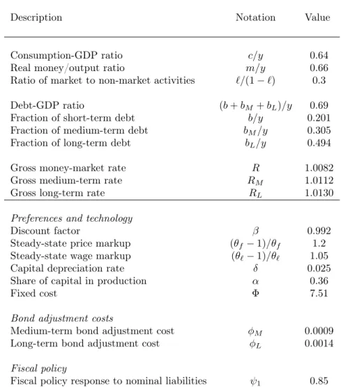
A number of parameters are calibrated to match the long-run values of the observables, consistently with the steady state relations of the model discussed in Appendix B.. I also fix some parameters because the dataset is uninformative for their estimation. Their values are reported in Table 1.
The discount factorβis calibrated from the long-run relation between inflation and the short-term rate. The depreciation rateδis 2.5% per quarter. Given a labor-income share in total output of 70%, I setαto 0.3. From an investment-output ratio equal to 0.2, I calibrate the fixed cost of production. The steady-state markups for prices and wages are calibration to 1.2 and 1.05, respectively, following Christiano, Motto and Rostagno (2007).
The bond-adjustment costs are not estimated because they are pinned down from the steady-state spreads between the yields. These parameters measure the share of income that households forego against a portfolio of assets. As argued in section 2.1.1, this generates positive holdings of different bonds in the long run. The economic intuition is that holding bonds of different maturities generates different opportunity costs in terms of output foregone. However, these bond holdings generate an array of yields. In the long run, the yields are tied to the opportunity costs of holding securities. Hence, for medium and long-term bonds, the adjustment costs are chosen to match average yields reported in Table 1. This givesφM = 0.0006andφL= 0.007.
The debt to GDP ratio in steady state is set to 45 percent. Data on the maturity structure of public debt are only at an annual frequency from Missale (1999) and from the OECD Dataset. In this paper, I use the OECD series available for the period 1995-2005. Since the statistics are reported on
a country basis, I take simple averages of maturity shares for the available EMU countries, namely Belgium, Germany, Italy, the Netherlands, Portugal and Spain. The ratio of public spending to GDP in steady state is 19.86 percent, while the tax to GDP ratio is 19.72 percent.
The feedback parameter ψ1 on the fiscal policy rule is of special interest because it largely affects
the determinacy properties of the model. I fix it to 0.92 which, within the range of reasonable values, should yield fiscal policy as ‘passive’ in the sense of Leeper (1991). In this sense, lump-sum taxes are not allowed to act independently from the outstanding stock of government’s liabilities, and are set to avoid an explosive path for public debt.
4.2
Prior distributions
The priors are reported in the second column of Table 2. The assumptions on the prior distributions are largely similar to those of Smets and Wouters (2003). All the variances of the shocks follow an inverted Gamma distribution with two degrees of freedom, so that the estimates fall in the region of positive values. The autoregressive parameters of the shocks have a Beta prior distribution with a small standard error. Most of the preference and technology parameters follow either a Normal or a Beta distribution with means consistent with previous studies. The intertemporal elasticity of substitution has a prior mean equal to one, consistently with the log utility in consumption that is typically used in estimated models (e.g. see Christiano, Motto and Rostagno, 2007). For the parameters on the adjustment cost functions for investment, prices and wages, I assumed a diffuse prior with starting values. These prior means are broadly in line with the available estimated models the U.S. economy (see Laforte, 2003 and Kim 2000), but lower than the values used in calibrated models of the Euro area (e.g. see Bayoumi, Laxton and Pesenti, 2004). After some preliminary estimation trials, I choose rather diffuse priors on the adjustment cost parameters between bonds and money. The model theory of imperfect substitutability between money and bonds suggests that the longer the maturity of a bond, the more households should be willing to ‘liquidate’ the bond. Hence the prior means should be such that vM > vL.10 Finally, there are rather standard priors on the parameters of the Taylor
rule. However, since the shape of the parameter regions that generate unique equilibria are unknown due to the new features of the model, the prior mean on the inflation coefficient is larger than usual, and the prior distribution has a higher standard deviation.
5
Alternative forecasting models
5.1
Competing DSGE models
I consider a number of variants of the ‘benchmark’ DSGE that allow to understand the contribution of model features to the predictive power. In the first set of competing models I remove various frictions from the benchmark specification and I re-estimate the resulting model. In particular, I estimation a version with flexible prices by fixingφP = 0.001, without adjustment costs between bonds and money
(vM =vL = 0), without consumption habits (h= 0), and without money target in the Taylor rule
(αm= 0). I also study the forecast performance of models with fewer exogenous shocks than for the
10It should be stressed that this restriction is not imposed in the estimation. Rather its plausibility will be confirmed
benchmark. I estimate model versions without shock to the inflation target (σπ = 0.0001), without
money velocity shock (σM = 0.0001), and without price markup shock (σP = 0).
To assess the importance of the key features of the benchmark DSGE model, I compare its out-of-sample forecasting performance with that of alternative models. In particular, I investigate how important the role of the feedback of the term structure to output is by considering a version of the model with strong separability in money and consumption, and without money growth in the Taylor rule. This amounts to estimating a model with the utility function
U(ct, ct−1, mt, `t) =E0 ∞ X t=0 βt pt 1 1−1/σ(ct−γct−1) 1−1/σ +mt Λ 1−χ(mt) 1−χ −`t Ψ 1 + 1/ψ` 1+1/ψ t . (56)
where γ is the elasticity of money demand, Λ is a parameter that helps matching the long-run money-output ratio, andm
t is an autoregressive money demand shock. I also include a consumption
preference shock with the standard autoregressive form. This shock is a source of exogenous variability for the stochastic discount factor, and helps matching the volatility of the rates without creating additional identification problems during the estimation. Optimal consumption plans are set according to [(1−γ)c]1/σλλˆt= β σ γ 1−γEtcˆt+1+ 1 σ γ 1−γˆct−1− 1 σ 1 +βγ2 1−γ ˆct, (57)
and the money demand equation becomes
Λm−χˆmt − Λχm−χ+ (vM +vL)λy ˆ mt+ β πλEt ˆ λt+1− β πλEtˆπt+1= λλˆt−vMλ y m ˆ bM,t−vLλ y m ˆbL,t. (58)
The central bank sets the policy rate according to the standard Taylor rule
ˆ
Rt=αRRˆt−1+ (1−αR) [ˆπt∗+απ(ˆπt−πˆt∗) +αyyˆt] +νtR. (59)
When estimating this model version with Bayesian methods, all the prior assumptions are the same as those of the benchmark model. Measurement errors are not used because they cause a drop in the value of the likelihood.
The following question of interest is whether the relation between the term structure and money demand conveys information relevant for understanding changes in output and inflation. Hence I estimate a version of the DSGE without medium and long-term rates. In other words, I remove the bond adjustment costs and the adjustment costs between bonds and money. The resulting DSGE is a prototype New Keynesian model with transaction costs between consumption and money, price and wage rigidity arising from quadratic adjustment costs. Bond supply shocks drop out of the model. The priors are the same as for the benchmark model.
De Graeve, Emiris and Wouters (2009) price the term structure by computing yieldsRˆn
bonds that are consistent with the expectations hypothesis ˆ Rnt = 1 nEt 1 X j=1 ˆ Rt+j−1. (60)
These term-structure yields are a function of the solution of the loglinearized model. The equations for the expectations-consistent yields can be appended to the DSGE model. The augmented DSGE is then estimated as a system using standard Bayesian methods. In order to match the volatility of the observed yields, and to capture time variation in term premia, measurement errors are included to the state-space form. In particular, the measurement equation now reads
" Yt Rn t # = " s Rn # + " ˆ st ˆ Rn t # + " 0 ηn t # (61)
Summing up, I augment the standard version of the New Keynesian model (without endogenous term structure) with two equations for the expectation-consistent pricing of bonds with maturity of 3 and 10 years. The model includes also measurement errors on medium and long-term yields.
For the estimation of all the models described in this section, I use the same prior assumptions of the benchmark. The priors for the measurement errors of the model of De Graeve, Emiris and Wouters (2009) are as follows. The standard deviations of both shocks have a uniform prior with mean 1.5 and standard deviation 1.5. The correlation of the measurement errors has a uniform prior with mean 0 and standard deviation 0.8.
5.2
Competing unrestricted models
I compare the out-of-sample performance of the benchmark DSGE model with that of a VAR system
Φ(L)Yt= Φ +vt (62)
where Φ(L) = Ip−Π1L . . .−ΠkLk, with the back-shift operator LYt = Yt−1. The disturbances
vtp(0,Σv) are independent across time. The VAR is estimated on the twelve series that are used to
estimate the DSGE.
The prior proposed by Litterman (1986) will be used on the dynamic coefficients inΠ, with the following default values on the hyperparameters: overall tightness is equal to 0:3, and cross-equation tightness is set to 0.2 and a harmonic lag decay with a hyperparameter equal to one. I use the non-informative prior|Σb|−(p+1)/2forΣv. The posterior distribution of the model parameters and the
forecast distribution of the endogenous variables were computed numerically using the Gibbs sampling algorithm in Kadiyala and Karlsson (1997). I report only the results from the VAR and BVAR with three lags. The forecasting results are similar across lag-lengths, with slight improvements delivered by the models with three lags.
6
Forecast accuracy criteria
The predictive performance of the model is evaluated on rolling forecasts from the DSGE model against a variety of competing models. In practice, each model is estimated until 2002:4. The forecast
evaluation starts in 2003:1. The models are re-estimated each quarter by updating the information set with one data point. The dynamic forecast distribution is then computed. The procedure continues until no data are available to evaluate the one period ahead forecast.
In this paper, I consider evaluation criteria for both point and density forecasts. Denote by
et(h) =Yt+h−Yˆt+h|t the h-step ahead error of the posterior mode forecast Yˆt+h|t at timet. The
standard measure of forecast accuracy is the usual root mean squared error (RMSE)
RM SEi(h) = v u u tN−1 h T+Nh−1 X t=T e2 i,t(h) (63)
whereei,t is thei-th element ofet(h), andNh denotes the number ofhstep ahead forecasts.
I also consider a multivariate measure of forecast accuracy based on theh-step ahead mean squared error matrix ΩM(h) =Nh−1 T+Nh−1 X t=T ˜ et(h)˜et(h)0 (64)
with ˜et(h) := M−1/2et(h). The term M indicates a scaling matrix acts as a scaling matrix that
accounts for the differing scales of the forecasted variables. A number of scalar valued multivariate measures of forecast accuracy are used in the literature. In this paper, I use the log determinant statisticlog|ΩM(h)| and the trace statistictr|ΩM(h)|. I setM equal to a diagonal matrix with the
sample variances of the time series based on data until 2002:4 as diagonal elements. With M equal to a diagonal matrix, the trace statistic reduces to a simple weighted average of the RMSEs of the individual series.
I also evaluate the accuracy of density forecasts of the competing models. For that purpose, I use the log predictive predictive density score test of multivariate forecast density. The log predictive density score of theh-step ahead predictive density is
St(Yt+h) =−2 logpt(xt+h) (65)
where the termpt(·)denotes the forecast distribution. Under the normality assumption, we have that
St(Yt+h) =klog(2π) + log|Σt+h|t|+ (Yt+h−Y¯t+h|t)0Σ−t+1h|t(Yt+h−Y¯t+h|t), (66)
with the posterior mean Y¯t+h|t and posterior covariance matrixΣt+h|t of theh-step ahead forecast
distribution. The average log predictive density score is
S(h) =Nh−1
T+Nh−1
X
t=T
St(Yt+h). (67)
6.1
Tests of predictive ability
The starting point for testing the forecasting power of the models discussed in this paper is the test of Diebold and Mariano (1995). This is a test of equal predictive ability between two competing models. Denote by {ei,t}nt=1 and {ej,t}nt=1 the forecast errors of two models i and j. The loss differential
between the two forecasts can be written as
dt:= [g(ei,t)−g(ej,t)] (68)
whereg(·)is the loss function.11 If{d
t}nt=1is covariance stationary and has no long memory, the sample
mean loss differentiald¯= (1/n)Pn
t=1dt is asymptotically distributed as
√
n( ¯d−µ)→d N 0, V( ¯d).
Under the null of equal predictive ability, Diebold and Mariano (1995) propose the test statistics
DM := ¯d/
q
ˆ
V( ¯d) ∼ N(0,1). As stressed by Harvey, Leybourne and Newbold (1997), the DM
test suffers from the oversize problem typical of small samples. For this reason, Harvey, Leybourne and Newbold (1997) propose a modified DM statistics that is obtained by multiplying the standard statistics by a correction factor
M DM :=
r
[n+ 1−2m+n−1m(m−1)]
n DM, (69)
wheremis the forecast horizon, and nis the length of the evaluation period.
White (1980) introduces a test for reality check — theRC test — that checks whether a specific forecasting model is outperformed by an alternative set of models according to a loss function. Let
LYˆk,t
denote the loss function for the prediction for modelk, fork= 1, . . . l. The relative predictive performance of the benchmark model0 with respect to the competing models can be computed as
fk,t=Lt,0− Lt,k. (70)
Iffk,t is stationary, we can define the expected relative performanceE[fk,t]. The testing procedure
amounts to checking that none of the competing models outperforms the benchmark under the null hypothesis
H0: max
k=1,...lE[fk,t]≤0. (71)
The rejection of the null implies that at least one competing model produces better forecasts than the benchmark. The test statistics is
Tn:= max
k=1,...l n
1/2¯
fk,n. (72)
Hansen (2005) stresses two issues with the distribution of Tn, namely that it is not unique under
the null and that it is sensitive to the specification of poor models. Since the distribution is not unique, it is important to obtain a consistent estimate of thep−value along with an upper and a lower bound. Hansen (2005) proposes to test the null hypothesis
H0: max k=1,...l E[fk,t] q var n1/2¯ fk,n ≤0. (73)
The test statistics has the form ˜ Tn:= max k=1,...l n1/2¯ fk,n q ˆ var n1/2¯ fk,n (74)
where var(ˆ ·) denotes an estimate of the variance obtained by bootstrap. The resulting test for super-predictive ability — denoted as SP A — includes the test for reality check as a special case. The upper bound for thep−value arises from a conservative test where all the competing models are assumed to be as good as the benchmark in terms of expected loss —SP Ac. TheSP Altest is instead
based onp−values that assume that the models with bad performance are poor models.
7
Results
7.1
Bayesian estimates
The posterior modes from the estimation of the ‘benchmark’ model outlined earlier are reported in the third column of Table 2.12 The estimates of the intertemporal elasticity of substitution are closer
to the lower range of values used in the business cycle literature (e.g. see Rotemberg ad Woodford, 1992). Households have a degree of habit formation at the mode lower than hat is obtained by Smets and Wouters (2003). The labour supply elasticity is estimated consistently larger than one. The relation between the parameters of the money-bond adjustment costs is consistent with the relation suggested by the theory. Their estimates are of magnitude close to the calibration proposed by Marzo, Söderström and Zagaglia (2008) for the U.S. The estimates of the coefficients in the Taylor rule deliver a high degree of policy inertia, a strong reaction to inflation, and a positive response to output, which is broadly in line with the estimates of Smets and Wouters (2003). The estimated coefficient of the money growth target is statistically significant, thus corroborating the results of Andrés, López-Salido and Vallés (2006). However, it is lower than what the estimates available from the literature. The estimates of the adjustment cost parameters of prices and wages are much higher than those of Kim (2000). The posterior estimates for parameter on the investment adjustment costs can be reconciled with those of Christiano, Eichenbaum, and Evans (2005). Most of the autoregressive shocks have a degree of persistence lower than the prior mean, with the exceptions of the labour supply and investment shocks. Finally, the posterior modes of the standard deviations of the shocks are on average larger than those obtained by Christiano, Motto and Rostagno (2007).
Table 2 also includes the posterior modes for models with flexible prices, no adjustment costs between bonds and money, no consumption habits, and no money growth target in the Taylor rule. Table 3 reports the posterior modes for models without inflation target shock, without money demand shock. The results that there are no major changes to the benchmark posterior modes.
Table 4 details the posterior estimates for the other variants of the benchmark DSGE model. The fourth column reports the posterior modes of the model without money demand feedback. Both the intertemporal elasticity of substitution and the labour supply elasticity are higher than under the benchmark estimates. However the model displays a larger degree of rigidity both in the goods and in
12The validity of the results from Bayesian estimation rests on the convergence of the Markov chain. I check for
convergence by monitoring plots of the draws from the Markov chain, and by computing two diagnostic tests. I use the CUSUM test of Bauwens et al. (1999) and the separated partial means tests of Geweke (2005, p. 149). All these criteria indicate that the Markov chain converges without problems.
the bond markets. The elasticity of money demand is about twice as large as the estimates of Andrés, López-Salido and Vallés (2006). This can be due to a variety of reasons. It should be estimated that the model of Andrés, López-Salido and Vallés (2006) does not include wage frictions, and that it is estimated only using a small number of series and includes four structural shocks.
The fifth column of Table 4 shows the estimates of the New Keynesian model without term structure. This framework is characterized by higher intertemporal elasticity of substitution. This suggests that, by simplifying the portfolio allocation problem and removing frictions, households can use resources in a more flexible way. At the same time, there is a higher degree of habit formation. The estimated labour supply elasticity becomes lower because wages are slightly more flexible, though the degree of indexation to the inflation target rises. From the perspective of the central bank, the estimated response to inflation falls. This happens because price setters face lower adjustment costs when changing nominal prices.
The last column of Table 4 includes the estimates of the model of De Graeve, Emiris and Wouters (2009). The results show that the expectations-consistent restrictions cause a number of parameter estimates to change with respect to the benchmark. The parameter on the investment adjustment cost becomes almost six times as large as the benchmark. Furthermore, the estimated shocks are less persistent and more volatile than the benchmark.
7.2
Forecast evaluation
7.2.1 Univariate accuracy measures
The forecast evaluation statistics are computed by estimating the models until December 2002. The forecast evaluation starts in January 2003. As stressed by Diebold, Piazzesi, and Rudebusch (2005) and Rudebusch, Sack, and Swanson (2007), the challenge of the macro-finance literature consists in modelling jointly the macroeconomy and the term structure of interest rates. Therefore, the forecast evaluation application will focus on both the term structure yields, and the real variables.
Figure 2 plots the root mean squared errors for forecasts up to 12 quarters ahead. The competing models are a VAR(3), a BVAR(3), and a random walk.13 With respect to macro variables, the
DSGE model of the term structure generates the best predictions for inflation and output over all the horizons. Its performance is close to the one of the best model for both consumption and the monetary aggregate. The model does not perform as well for investment, employment and wages. The predictive power of the DSGE model for the bond yields is close to best at the longer horizons, as the VAR models tend to do better for up to 4 months ahead.
Figure 3 reports the root mean squared errors of the versions of the DSGE without various frictions or without exogenous shocks. Several points of interest emerge. The benchmark specification achieves the best predictive performance for most of the variables, with the exception of investment and employment. Removing the money velocity shock, the adjustment costs between bonds and money, or the money target in the Taylor rule worsens the predictive performance for M3. The models without inflation target shock and without price stickiness generate forecast errors larger than those of the benchmark model. However, the decline in predictive performance is rather small. This is somewhat at odds with what the macro-finance literature suggests, which suggests that nominal price rigidities
13I use a VAR and a BVAR of order 3 for illustrative purposes. In fact I find that the predictive performance is
are the key driving forces for bond prices (e.g., see Gurkaynak, Sack and Swanson, 2005 and Emiris, 2006). Taken at face value, this suggests that the models that disregard the feedback might put excessive weight on the role of nominal rigidities for term structure yields.
Figure 4 reports the forecast statistics of the standard New Keynesian model without the term structure. The model with the term structure predicts both output and inflation more accurately than the standard New Keynesian model. This result is of interest especially because the model without the term structure is a good forecasting model as it delivers a good predictive performance with respect to both the random walk and the BVAR. These findings suggest that the modelling strategy for the term structure pursued in this paper generates information for predicting output and inflation that is not contained in the standard model without the term structure.
Figure 5 plots the out-of-sample forecast statistics of the benchmark model and the model without money demand feedback. Two observations arise. First, failing to account for the relation between output and money with an endogenous term structure worsens the misspecification of money demand, which explains the large forecast failure of the model without money demand feedback for M3. Second, the benchmark model predicts the term structure yields better than the model without money feedback. This finding is surprising in light of the fact that the model with money in the utility includes the additional shock to consumption preferences. This allows to discriminate between exogenous variations in consumption and those of money demand, and should provide additional fitting ability. The overall lesson is that the relation between output and money featured in the benchmark model is supported by its forecasting performance.
It is also instructive to compare the predictive performance for M3 of the model without money demand feedback and the standard New Keynesian model of Figure 4. The root mean squared errors in the model without money feedback are twice as large as those of the standard model. This could arise if the modelling strategy for the endogenous term structure was a source of under-fitting. In additional forecasting exercises not reported here, a model with no money demand feedback and no endogenous term structure loses further predictive ability for M3 with respect to a model without feedback and endogenous long-term rates, without major deteriorations in the forecasting ability of the remaining variables. These considerations suggest that the money demand feedback captures relevant features of the monetary transmission mechanism.
Figure 6 plots the out-of-sample forecast statistics for the model De Graeve, Emiris and Wouters (2009). It is evident that the additional restrictions imposed by the expectation-consistent pricing relations create a general deterioration in the predictive power of the model, in particular for output and M3. The pattern of forecast errors for inflation, though, is rather close to the one of the best forecasting model. This explains why the forecasts of the model of De Graeve, Emiris and Wouters (2009) for the money market rate are still acceptable. Overall, these findings indicate that the bond market frictions behind the endogenous term structure of the benchmark model yield desirable empirical properties that cannot be generated by a competing pricing for bonds.
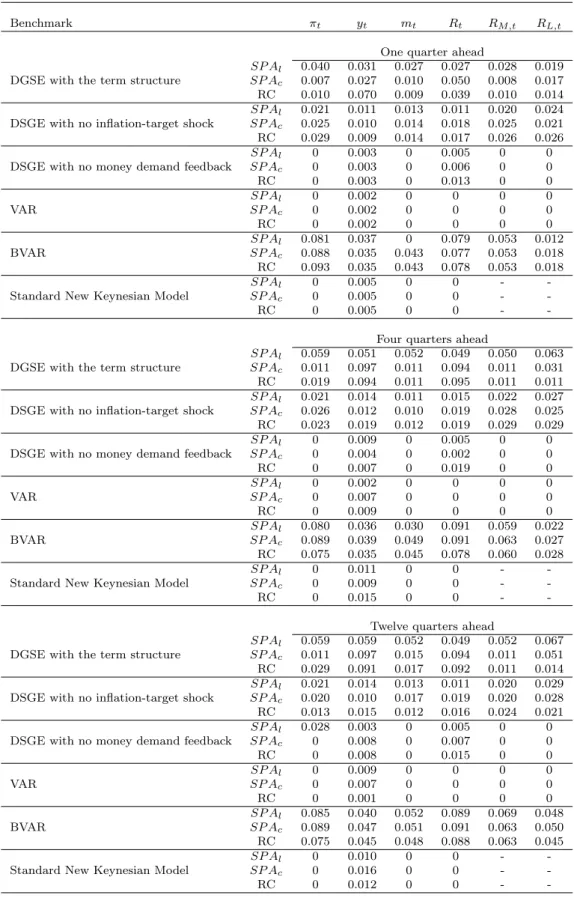
7.2.2 Multivariate accuracy measures
Table 5 reports the multivariate accuracy measures, the log determinant and the trace statistics of the mean squared error matrix for 3 forecast horizons (1, 4 and 12 quarters ahead). For comparison purposes, the forecasts are shown for two sets of variables. The first group of variables, including inflation, output, money and the short-term rate, allows to compare all the models. The second group
consists of the three term structure yields. For this case, the DSGE model without long-term rates is excluded from the comparison. The results from multivariate accuracy confirm the findings from the univariate measures on several points. The BVAR is the best predictive model both for the real variables and for the term structure yields. The benchmark DSGE performs better than the model variants without frictions. There is only one exception though. The log predictive density score suggests that the model of De Graeve, Emiris and Wouters (2009) beats the benchmark DSGE only for forecasts of real variables at 1 quarter ahead. In terms of log determinants and trace statistics, the third ranking models are those without money demand feedback ranks at a 1 quarter horizon, and that with no inflation target shock at 4 and 12 quarters ahead.
In order to investigate further these findings, I study the contribution of the root mean squared errors to the log determinant statistics. As noted by Andrés, López-Salido and Vallés (2006), a singular value decomposition can be applied to the matrix ΩM(h)as ΩM(h) =VΛV0 where V0V =Ik is the
matrix of eigenvectors, andΛ = diag(λ1, . . . λk)is a diagonal matrix with ordered eigenvaluesλ1≥λk.
This also suggests thatlog|Ω|=Pk
j=1logλj andtrace(Ω) =P
k
j=1λj. In other words, since the first
eigenvalue is the variance of the first principal component, λ1 represents the variance of the linear
combination of time series that produces the highest forecast error variance.
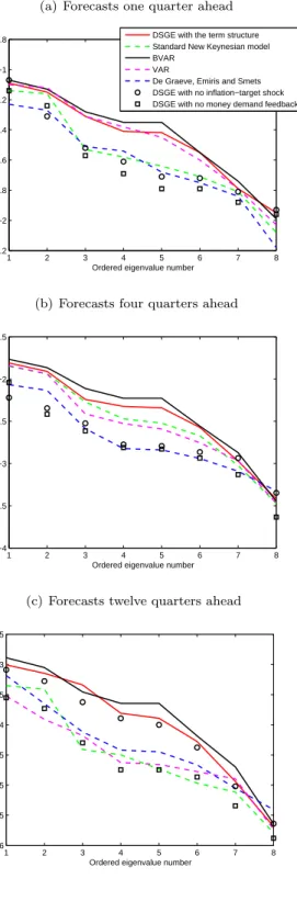
Figure 7 plots the ordered eigenvalues (in logarithm) from the decomposition of the log determinant for the prediction of four variables (output, inflation, money and the short rate).14 I compare the
DSGE model of the term structure with six competing models, namely the VAR, BVAR and four general-equilibrium models. Two main observations arise. First, independently from the predictive horizon, the contribution of the eigenvalues discriminates largely between two sets of models, where one group performs better than the other in terms of log determinant statistics. Second, the differences between log determinants do not concentrate on the smaller eigenvalues, but are present also among the largest eigenvalues. These considerations indicate that the DSGE with the term structure has a performance superior to one of the other structural models because it predicts variables that account for a sizeable portion of the principal components.
7.2.3 The statistical significance of univariate forecasts
Table 6 reports the results of the tests of Diebold and Mariano (1995). These tests are computed with the DSGE model of the term structure as the benchmark. Its advantage over the the competing general-equilibrium models is statistically-significant for all the horizons. The sign of the DM statistic is always negative, implying that the benchmark’s loss is lower than the one implied by the competing models. Only the BVAR beats the benchmark model for predicting all the variables.
Table 7 reports the p-values from the tests for reality check and super-predictive ability. The loss function used in the tests is the root mean squared error reported in Figures 2-6. Each model is treated as benchmark at the time and is evaluated against all the others. For every model, the rows present the p-values, where RC indicates the reality check and SP Ac and SP Al refer, respectively, to the
consistentp-values of Hansen (2005) and the lowerp-values. Like in White (1980), these probabilities are computed through the bootstrap procedure of Politis and Romano (1994), with a re-sampling size of 5000 and a block length of 0.2.15 The lowp-values indicate that there is at least one competing
14The pattern of the ordered log eigenvalues for the forecast of the three term structure yields is similar to the one
diplayed in Figure 7, and is not reported for brevity.
model which performs better than the benchmark. All the bivariate comparisons reject the null. This confirms that there is no single best model. Thep-values for the BVAR model are, on average, higher than those of the other models. However, also in this case, there are no rejections at standard confidence levels.
8
Conclusion
A large number of studies investigates the role of monetary policy and, in particular, changes in the central bank’s inflation target for the dynamics of government bond yields. With few exceptions, the empirical literature ignores the policymakers’ common view that the yield curve is a key part of the monetary transmission mechanism. The available macro-finance models are also been used for forecasting the term structure of interest rates.
In this paper, I use Bayesian techniques to estimate the general equilibrium model of Marzo, Söderström and Zagaglia (2008) where long-term rates affect both real and nominal variables. The theoretical framework is based on the ‘theory of preferred habitat’ of investors, which characterizes the portfolio allocation problem as a sluggish decision of agents over different market segments. The model includes frictions in the money and bond market to generate equilibrium holdings of several bonds. Following the approach of Adolfson, Lindé and Villani (2007), I then study predictive performance by comparing several forecast accuracy measures across different DSGE models.
The results show that the model presented in this paper compares favorably with respect to unrestricted models (VAR and BVAR) for predicting both real and nominal variables, including the term structure yields. The model also fares well in comparison with the DSGE model of the term structure of De Graeve, Emiris and Wouters (2009), where long-term rates are priced consistently with the expectations hypothesis. These findings suggest that the model of the feedback from the term structure captures relevant properties of the data, thus generating statistically-superior forecasts.
Numerous extensions to the current analysis can be envisaged. In a work in progress, I relax the assumption on the available information set that is currently used in the estimation of the benchmark DSGE model. In particular, I employ a large panel dataset with macroeconomic and bond yield data along the lines of Boivin and Giannoni (2006). This suggests that it would be interesting to enlarge the range of competing models by including the no-arbitrage factor VAR of Moench (2008). An additional dimension of interest is the misspecification of the benchmark DSGE. In this sense, I am planning to apply the methods proposed by Del Negro and Schorfheide (2004).
A
Loglinearization
A.1
Households
γ σ(1−γ) −1/σ−1 cˆct−1− 1 σ 1 +βγ 2 (1−γ)−1/σ−1+ 3λmc m 2 ˆ ct +γ σβ(1−γ) −1/σ−1 Etcˆt+1 = 1 +m c m2 λλˆt−3λm c m 2 ˆ mt+ 3 2λ mc m 2 ˆ mt (A1) Ψθ` w` 1/ψˆ` t+ Ψθ` w` 1/ψ−λθ `` ˆ θ`,t+ (1 + 1/ψ)θ` w` 1/ψ+λ(1−θ `)` ˆ `t − ψθ` w` 1/ψ+λφ wπ2(1 +γw)−λφwγwπ∗π−βλφw(1 + 2γw)−2βλφwπ∗π ˆ wt −λ[φwγwπ(π−π∗)−(1−θ`)`] ˆλt +λφwγwπ∗πˆπ∗t− λφw(π∗(1 +γw)−γwπ∗π)−βλφw(1−γw)π2 ˆ πt +βφwλφwπ∗πEtπˆt∗+1+λφw π2(1 +γw)−γwπ∗πwˆt−1+λφw(1−γw)π2ˆπt−1 +βφwλγw(π−π∗) ˆλt−1+βλφwγwπ(π−π∗)Etλˆt+1 +βλφw(1 + 2γw)π2−2γwπ∗πEtwˆt+1+βλφw(1 +γw)π2−γwπ∗πEtπˆt+1 (A2) β πλEt ˆ λt+1− β πλEtπˆt+1= 3mc m 3 + (vM +vL)λy ˆ mt +λλˆt−3m c m 3 ˆ ct−vMλ y m ˆ bM,t−vLλ y m ˆb L,t−m c m 3 ˆ mt (A3) ˆ Rt+Etλˆt+1−Etπˆt+1= ˆλt (A4) βRM π λ ˆ RM,t+βλ R M π +φSy Etˆλt+1−β RM π λEtˆπt+1 +βφSλyEtyˆt+1+ 3βφSλyEtˆbS,t+1= λ 1 + 3 2φSy ˆ λt+ 3 2λφSyˆyt−3φSλy ˆbM,t −1 + 3φSλy(1 +β)−λvMy m bM ˆ bM,t+λvM m bM ymˆt (A5) βRL π λ ˆ RL,t+βλ R L π +φLy Etˆλt+1−β RL π λEtπˆt+1 +βφLλyEtyˆt+1+ 3βφLλyEtˆbL,t+1 = λ 1 + 3 2φLy ˆ λt+ 3 2λφLyyˆt−3