1
Concentrated Solar Power: actual performance and foreseeable future in high penetration scenarios of renewable energies
Carlos de Castroa,b,* Iñigo Capellán-Pérezb September 2018
aApplied Physics Department, Escuela de Arquitectura, Av Salamanca, 18, University of Valladolid, 47014, Valladolid, Spain. ccastro@termo.uva.es
bResearch Group on Energy, Economy and System Dynamics, University of Valladolid, Spain
Author Accepted Manuscript from the paper published in the journal “BioPhysical Economics and Resource Quality”:
Carlos de Castro, Iñigo Capellán-Pérez: “Concentrated Solar Power: actual performance and foreseeable future in high penetration scenarios of renewable energies”. September 2018. BioPhysical Economics and Resource Quality (2018) 3:14. https://doi.org/10.1007/s41247-018-0043-6
Abstract
Analyses proposing a high share of Concentrated Solar Power (CSP) in future 100% renewable energy scenarios rely on the ability of this technology, through storage and/or hybridization, to partially avoid the problems associated with the hourly / daily (short-term) variability of other variable renewable sources such as wind or solar photovoltaic. However, data used in the scientific literature are mainly theoretical values. In this work, the actual performance of CSP plants in operation from publicly available data from 4 countries (Spain, the USA, India and UAE) has been estimated for 3 dimensions: capacity factor, seasonal variability and Energy Return on Energy Invested (EROI). In fact, the results obtained show that the actual performance of CSP plants is significantly worse than that projected by constructors and considered by the scientific literature in the theoretical studies: a capacity factor in the range of 0.15-0.3, low standard EROI (1.3:1-2.4:1), intensive use of materials –some scarce-, and significant seasonal intermittence. In the light of the obtained results, the potential contribution of current CSP technologies in a future 100% renewable energy system seems very limited.
© 2017. This manuscript version is made available under the CC-BY-NC-ND 4.0 license http://creativecommons.org/licenses/by-nc-nd/4.0/
2
Table of contents
1. Introduction ... 2
2. Concentrated solar power plant technologies ... 5
3. Capacity factor (CF) ... 6
4. Monthly/seasonal variability ... 8
5. EROI ... 13
5.1. EROI expression ... 13
5.2. Energy Used by CSP system (EnUtot) ... 14
5.2.1. Scenarios ... 17
5.2.2. Current EnU of CSP plant ... 18
5.2.3. EuN of CSP plants in high RES penetration scenarios ... 19
5.3. The g factor (average efficiency in the transformation of primary energy to electricity and the quality of the energy) ... 20
5.4. Estimation of EROI ... 21
6. Discussion and conclusions ... 24
Acknowledgements ... 26
References ... 26
Appendix A ... 32
Appendix B ... 33
1.
Introduction
The transition to Renewable Energy Sources (RES) is an indispensable condition to achieve sustainable socio-economic systems. Most governments are developing policy frameworks to promote the penetration of renewable energy sources to improve energy security (increasingly threatened by the depletion of fossil fuels), while mitigating emissions to limit anthropogenic climate change and other negative externalities of conventional energy sources (Capellán-Pérez et al., 2014; IPCC, 2014; Johansson, 2013; REN21, 2015; WEO, 2014). Among renewables, wind and solar are estimated to have the greatest potential (de Castro et al., 2013; IPCC, 2011; Smil, 2010), with projections often assuming that the resource base provides no practical limitation if adequate investments are forthcoming (e.g., (IEA and IRENA, 2017; IPCC, 2011)). At the same time, wind and solar are the RES most critically affected by the intermittency of the source in the short (e.g. hours, day/night), medium (days/weeks) and long-term (e.g. winter/summer, annual) (Capellán-Pérez et al., 2017b; MacKay, 2013; Trainer, 2017a, 2013, 2012, 2010; Wagner, 2014). In this context, concentrating solar power (CSP) with thermal energy storage (TES) can partially compensate for the short-term variability of other RES due to its ability to store energy and dispatch energy following the demand. Due to its ability to provide an hourly/daily flexible capacity, CSP is expected to complement PV and wind, substantially increasing their penetration potential, especially in locations with adequate solar resources. The performance of CSP is also enhanced when coupling the plant to a back-up
3
system, typically natural gas (Denholm and Mehos, 2015; Olivares, 2016; García-Olivares et al., 2012; Jacobson and Delucchi, 2011; NREL, 2012). On the other hand, CSP plants are more expensive (IEA and IRENA, 2013; IRENA, 2018; Trainer, 2017b; Turchi, 2010) and, at present, represent a less universal solution than other RES in general and than PV in particular. This is because: (1) they only use direct irradiance (DNI) (PV also uses diffuse irradiance); (2) they require higher levels of irradiance with low cloudiness to be economically optimal, most suitable locations corresponding to arid zones; and (3) they adapt less well to terrain unevenness (Deng et al., 2015; Hernandez et al., 2015).1 Thus, CSP investments are expected to be profitable just when a relatively high renewable penetration is targeted in the electricity mix (Brand et al., 2012).
Globally, the installation of new capacity has grown at a pace of over 30% per year between 2005-2015, but in 2015 the growth was 9.7%, and in 2016 just 2.3% (REN21, 2017, 2016). Also, for the first time, all of the facilities added in 2015 and 2016 incorporated TES capacity, a feature now seen as central to maintaining the competitiveness of CSP through the flexibility of hourly/daily dispatchability (REN21, 2016, 2017). At the end of 2015 there were over 4.8 GW of CSP in operation globally, which produced almost 10 TWh in that year (as opposed to over 250 TWh produced by all solar technologies) (IRENA db, 2017); <0.04% of the global electricity produced in that year (BP, 2017). Spain and the USA at present account for most of the CSP installed power (~80%); however, facilities are under construction in several countries such as Australia, Chile, China, India, Israel, Mexico, Saudi Arabia and South Africa. Thus, it is commonly expected that this technology will spread over the next few years in those countries with high irradiance levels (REN21, 2016, 2017). However, the global deployment level of CSP is still currently low and uncertain.
Due to the aforementioned factors, CSP with TES is thus usually seen as a key technology to design or approach 100% RES power systems. Table 1 shows the estimated contribution of CSP by different studies in the literature proposing global 100% RES scenarios (Delucchi and Jacobson, 2011; García-Olivares, 2016; Greenpeace et al., 2015; Jacobson et al, 2016; Jacobson and Delucchi, 2011; WWF, 2011). These studies typically assume that large quantities of electricity could be technically transported on a continental scale between areas of high renewable resources (e.g. solar from deserts and wind from marine platforms) to the regions of consumption.2 In terms of energy generation, these studies project generation from CSP to range from 1 to 5 TWe (9,000 – 44,000 TWh/yr or 30-160 EJ/yr), which is between 40% and almost 2 times the current global electricity generation by all sources. The projected share of CSP ranges between 12% (WWF, 2011) to 42% (García-Olivares, 2016) of the total energy generation. The capacity factor (CF, i.e., the ratio of an actual electrical energy output over a given period of time to the maximum possible electrical energy output over the same amount of time) considered by these studies ranges from 0.31 to 0.75 and is thus supposed to be around 2 to 3 times bigger than the CF of other RES, such as wind and solar PV respectively.
1 Additionally, restrictions on water use in arid regions that often have the most appropriate solar
resources for CSP would reduce plant efficiency due to the implementation of dry-cooling technologies.
2 However, these large scale intercontinental infrastructures are challenged by geopolitical and
economic barriers, as well as concerns over energy and food security (for a detailed discussion, see (Capellán-Pérez et al., 2017b)).
4 CSP energy
generation
Total energy
generation Share CSP CF
Study TWe TWe %
(García-Olivares, 2016) 5 12 42 0.4-0.75
(Delucchi and Jacobson, 2011; Jacobson and Delucchi, 2011) 2.3 11.5 20 0.31 (Greenpeace et al., 2015) 1.6 9.7 16 0.63 (WWF, 2011) 1 8.3 12 0.46 (Jacobson et al, 2016) 1.8 11.8 15 0.53
Table 1: Contribution of CSP in global 100% RES scenarios. CF: power plant capacity factor.
Other studies focusing on scenarios of strong penetration of RES at country-level also assume a big participation of CSP when there are good solar irradiance resources. For instance, Lenzen et al., (2016) gives a 49% share of electricity production for a 100% RES electricity transition model for Australia (with plant CF of 0.3 without TES, and a CF of 0.6 with 15 hours of storage by TES). Elliston et al., (2012) also gives a 40% penetration share of CSP with CF of 0.6 for Australia; whereas NREL (2012) gives a share of 12% of electricity production (CF=0.51) for a 90% RES electricity penetration scenario for the USA.
Most studies in the literature usually apply theoretical assumptions for modeling RES systems that have been shown to overestimate the performance of real systems (Clack et al., 2017; Moriarty and Honnery, 2016; Trainer, 2017a, 2013, 2012, 2010). For example, for wind, Arvesen and Hertwich (2012) concluded that “there appears to be a general tendency of wind power LCAs to assume higher capacity factors than current averages from real-world experiences”. Boccard (2009) found that, despite the capacity factor of wind power usually being assumed to be in the 30–35% range of the name plate capacity, the mean realized value for Europe between 2003 and 2007 was below 21% (findings consistent through the period 2000-2014 (IRENA db, 2017)).
The energy return on energy invested (EROI), estimated for theoretical or particular plants, in particular for PV, has been contested when compared with the EROI of national RES systems, with a tendency to lower the expectations (Ferroni and Hopkirk, 2016; Palmer, 2013; Prieto and Hall, 2013; Weißbach et al., 2013). An ongoing discussion over this important issue is taking place at present (Ferroni et al., 2017; Raugei et al., 2017, 2015; Weißbach et al., 2014). However, to our knowledge, no study has to date focused on the real performance of CSP. In this work, we fill this gap in the literature by estimating the capacity factor, seasonal variations and EROI values of CSP plants in operation. Ultimately, the aim of the paper is to provide ground for discussion on the potential contribution of CSP to a 100% RES system.
The capacity factor is a parameter that critically affects the life-cycle analyses that estimate the energy and material requirements (such as the energy payback time (EPT) and EROI) as well as the environmental impacts (e.g. global warming potential, acidification, eutrophication, loss of biodiversity, noise, human and ecosystem toxicity, land requirements, etc.) and economic costs. For example, a comparison of the real capacity factor at global level of CSP could be quickly estimated using the aforementioned data for 2015 (IRENA db, 2017): an installation base of 4.4GW at the end of the year with an annual production of 9TWh; assuming that the new capacity was added uniformly throughout 2015, this would give a CF = 0.24, which contrasts with the usually considered values in the literature (range 0.25-0.75, depending on the technology and geographical location of the plant (Burkhardt et al., 2011; Corona et al.,
5
2016, 2014; García-Olivares, 2016; IEA and IRENA, 2013; Klein and Rubin, 2013; Lechón et al., 2008; Pihl et al., 2012; Turchi, 2010; Viebahn et al., 2011; Weinrebe et al., 1998), see Table 2 in section 3). This comparison suggests that similar discrepancies between theoretical and real performance to those existing for other RES might also be present for CSP.
The real performance of CSP is analyzed through the collection of publicly available data from 34 individual CSP power plants in operation in 4 countries (Spain, the USA, India and United Arab Emirates (UAE)) (IRENA db, 2017), which amounts to >40% of the total CSP power capacity installed in the world, as of the end of 2016, and the national-aggregated production of Spain. The obtained results are compared with the values used in the peer-review literature, the online global list of CSP projects from NREL (2017) and the data provided by the constructors of the power plants.
In a second stage, annual and monthly electricity production are analyzed for diverse CSP plants and a new indicator of performance for variable RES is proposed based on Capellán-Pérez et al., (Capellán-Capellán-Pérez et al., 2017b) called “Sv”3, defined as the ratio of the electricity generation from the worst month in a year versus the average monthly electricity generation in that same year, therefore, the lower the Sv, the higher the seasonal intermittence. This performance indicator will be compared with other variable RES for the Spanish and USA power systems.
In a third stage, we re-estimate the EROI of different CSP power plants studied in the literature, taking into account the real capacity factors previously found and recalculating the total Energy Used (EnUtot, the total energy used in the construction, operation and disposal of the CSP system), taking on board three key factors usually not considered in the literature in enough detail: (1) including most materials involved in the construction and operation of CSP plants; (2) the use of particular values of embodied energy in materials (MJ/kg) used by CSP and not common to other RES technologies; and (3) considering CSP technologies using abundant materials. Finally, in the light of the obtained results, the potential contribution of CSP in 100% RES systems is discussed.
The paper is organized as follows. Section 2 overviews the CSP technologies, while sections 3 to 5 review the performance factors of real CSP power plants in operation: capacity factor (section 3), monthly and seasonal variability and intermittence (section 4) and EROI (section 5). Finally, section 6 discusses the implications of the results.
2.
Concentrated solar power plant technologies
CSP is an electricity generation technology that uses heat provided by solar irradiation concentrated on a small area. Using mirrors, sunlight is reflected to a receiver where heat is collected by a thermal energy carrier (primary circuit), and subsequently used directly (in the case of water/steam), or via a secondary circuit to power a turbine and generate electricity. At present, there are four available CSP technologies: parabolic trough collector, solar power tower, linear Fresnel reflector and parabolic dish systems (Zhang et al., 2013). In this study, we refer to them as Parabolic, Tower, Fresnel and Dish technologies, respectively.
The CSP performance can be enhanced by the incorporation of two complementary technologies: Thermal energy storage (TES) and backup systems. Storage avoids losing the daytime surplus energy while extending the production after sunset. TES collects the excess
3 In Capellán-Pérez et al. (2017), Sv is called Seasonal Variation, that could be a rather confusing term;
here we use this performance factor in this sense: the more seasonal variation the lower Sv, or inversely, the more approaching Sv=1 the lesser seasonal variation of electricity production.
6
heat in the solar field and sends it to a heat exchanger, which warms the heat transfer fluid going from the cold tank to the hot tank. When needed, the heat from the hot tank can be returned to the heat transfer fluid and sent to the steam generator. A fuel backup system (typically based on natural gas) helps to regulate production and/or guarantee a desired generation capacity, especially in demand peak periods. CSP plants equipped with backup systems that produce electricity are called hybrid plants. For more information on CSP technologies see Zhang et al., (2013).
CSP plants produce electricity from a thermal process that can be supported by non-solar sources. Those plants that use natural gas as back-up can use it to preheat the thermal fluid or to maintain the heat of the molten salts or the material that can be used as storage; it can also use the natural gas to produce electricity. Some CSP projects propose to replace the use of natural gas with biomass so that they can be coherently classified as renewable sources (e.g., Borges Termosolar (Lleida, Spain) uses hybridization with biomass of forest residues and natural gas). The hybridization with natural gas increases efficiency and therefore the capacity factor (CF), defined here as the ratio of electric power supplied on average in a year by the power plant and the nominal capacity of the plant that we will take as the gross power of the turbine. The back-up with natural gas, and especially the use of storage, allows electricity to be generated relatively independently of the instantaneous solar radiation.
Since we intend to characterize CSP plants as renewable in a context of future scenarios of 100% RES, the output energy of the plant that we consider will be the net electric power produced from the solar field. In the case of hybrid plants with natural gas, if this produces electricity, the share of the production coming from the natural gas is deducted. In the event that natural gas is used to support the storage or to maintain the heat of the thermal fluid, that natural gas will be accounted for as self-consumption of the plant. The fact that many CSP plants use natural gas for the preheating of thermal fluid instead of electricity is somewhat paradoxical, if we take into account the fact that the plant produces electricity and is therefore connected to an electrical grid from which it could take that energy. However, these plants generally prefer to build a parallel gas network (sometimes kilometers away from a natural gas source) with all the energy and material costs involved.
As the solar efficiency of the hybrid system increases, it becomes more difficult to quantify the contribution of the support system, so the net electricity produced that we consider will be greater than what a pure renewable system would generate; therefore, we will probably be conservative/optimists in some of the estimates.
3.
Capacity factor (CF)
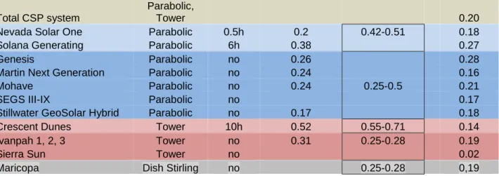
Table 2 shows the values of the capacity factor estimated from real production data (“Real CF” column) for different technologies and individual CSP plants from 4 countries (Spain, the USA, India and UEA) as well as for the complete CSP system of the USA and Spain. Subsequently, the obtained values are compared with: (1) the range values published in the scientific literature (column “Literature CF”), and (2) the foreseen CF by constructors (“Expected CF” column) as found in the NREL’s list of CSP plants (NREL, 2017) from the announced electricity production and the gross power of the plant or the construction companies’ websites or projects.
7
Tecnology Storage Expected CF Literature CF Real CF CSP in USA
Total CSP system
Parabolic,
Tower 0.20
Nevada Solar One Parabolic 0.5h 0.2 0.42-0.51 0.18
Solana Generating Parabolic 6h 0.38 0.27
Genesis Parabolic no 0.26 0.28
Martin Next Generation Parabolic no 0.24 0.16
Mohave Parabolic no 0.24 0.25-0.5 0.21
SEGS III-IX Parabolic no 0.17
Stillwater GeoSolar Hybrid Parabolic no 0.17 0.18
Crescent Dunes Tower 10h 0.52 0.55-0.71 0.14
Ivanpah 1, 2, 3 Tower no 0.31 0.25-0.28 0.19
Sierra Sun Tower no 0.02
Maricopa Dish Stirling no 0.25-0.28 0,19
CSP in
United Arab Emirates
Parabolic no 0.24 0.25-0.9 0.20 CSP in Spain Total CSP system Parabolic, Tower, Fresnel 0.25
Andasol 1,2,3, Granada parabolic 7.5 0.374 0.30
Valle 1,2, Cádiz parabolic 7.5 0.4 0.42-0.51 0.32
Enerstar Villena, Alicante parabolic no 0.228 0.25-0.5 0.16
Puerto Errado 1,2, Murcia fresnel 0.5h 0.185 0.22-0.24 0.15
CSP in India
Godawari Solar Project parabolic no 0.27 0.25-0.9 0.19
Range - 0-10h 0.2-0.5 0.25-0.75 0.15-0.30
Table 2: Estimates of the CF of several individual CSP plants, sets of plants and global USA and Spanish CSP systems: expected values from the industry, values used in the scientific literature and the results obtained in the work for real plants. The type of technology has been indicated as well as if plants have storage (molten salts).
The “Real CF” column is the one calculated for the net solar production: for the USA Total, we take the period Oct 2016-Sep 2017 (the last year of data from EIA (US EIA db, 2018)) (plants that at present are not in operation are excluded, also the Still Water plant due to lack of data for the year 2017 as of January 2018). For Maricopa, we take 11 months of 2010; this demonstration plant was decommissioned in 2011. For SHAMS, we take the average of 2014, 2015 and 2016 (Alobaidli et al., 2017; Sanz, 2017). For the Sierra plant (closed at present), we take the average over its (short) life time. For the Godawari plant in India, we take the monthly data from April 2015 to March 2016 (Solanki, 2016). For the Spanish CSP system, the calculation refers to the year 2017, except December (REE, 2018). For the individual Spanish plants, data are for 2016 from the Ministry of Energy (Ministerio de Energía, 2018). All data are
8
net solar production, which for hybrid plants is estimated by deducting 4.4%4 of the electricity production attributable to natural gas, in accordance with Spanish national legislation (Ministerio de Industria, Energía y Turismo, 2014), as well as assuming 10% self-consumption. The column of “Literature CF” refers to the range that has been found in the scientific literature. For the parabolic technology with storage (Burkhardt et al., 2011; Corona et al., 2014; Lechón et al., 2008; Pihl et al., 2012; Turchi, 2010; Viebahn et al., 2011), for the parabolic technology without storage (IEA and IRENA, 2013; Klein and Rubin, 2013; Weinrebe et al., 1998), for Tower technology with storage (Corona et al., 2016; IEA and IRENA, 2013; Lechón et al., 2008; Pihl et al., 2012; Viebahn et al., 2011), for Tower technology without storage (IEA and IRENA, 2013), for Fresnel technology (IEA and IRENA, 2013), and for Dish Stirling technology (García-Olivares, 2016; IEA and IRENA, 2013). For the UEA SHAMS plant and the Godawari India plant, García-Olivares (García-Olivares, 2016) considers 0.75 in subtropical deserts and quotes Trieb (2006) who gives 0.9 as possible for these latitudes.
Table 2 shows that the CF of real plants currently in operation is in the range of 0.15-0.3 and this is a lower value than those expected by the industry (0.2-0.5) or those usually used in the academic literature (0.25-0.75). In general, the CF of the Spanish plants is better than that of the USA ones (despite a lower average solar irradiance in Spain). This may be due to the fact that Spanish plants are usually hybridized with natural gas and the method applied to estimate the net renewable electricity produced is probably underestimating the natural gas contribution.
In the light of the obtained results, the current average CF level of CSP plants in the present electricity system (with low penetration of RES variables) is around 0.2 for plants without storage and 0.25 for plants with storage.
4.
Monthly/seasonal variability
CSP with storage and/or hybridization can partially avoid the problems associated with the hourly/daily (short-term) variability of other variable renewable sources, such as wind or PV. In order to investigate the scale of medium and long-term variability, the monthly output of some real CSP plants currently in operation is reported and compared with the variability of other intermittent RES.
Figure 1 shows the monthly electricity generation of the Genesis solar plant (USA) from November 2013 to September 2017, with large fluctuations between summer and winter. The same pattern is identified for the 7 plants SEGSIII-IX (Figure 2). In the latter, the fact that the back-up power from natural gas is mainly used in high productivity months, i.e., exacerbating the seasonal variability, is also visible.
4 4.4% = 15%·0.2907, 15% being the legal maximum of primary energy to be supplied by gas, and 0.2907
the efficiency factor of gas combustion. Assuming that the maximum has been reached, this is reasonable, given that most CSP plants in Spain have been penalized in the past for surpassing the 15% level (CNMC, 2016).
9
Figure 1: Monthly production (data from the EIA) of the Genesis plant. It is a plant without storage and without hybridization, although it consumes approximately 2% of what it produces with natural gas that serves to keep the thermal fluid hot. This natural gas not only prevents the possibility of that fluid solidifying, but also helps to activate the electrical production in the first hours of the morning. Note that, between monthly minimums and maximums, there may be a difference factor of more than 5.
We apply the performance indicator Sv to evaluate the variations of output along the year. This indicator was defined in Capellán-Pérez et al., (Capellán-Pérez et al., 2017b) at a theoretical country-level, and here it is applied at plant-level. Sv is a sensitive indicator to be taken into account when assessing a hypothetical mix of high penetration of renewable energies, as it gives an idea of the fluctuations that must be dealt by the whole system when it is lower than 1. In particular, the Sv can be used to estimate the overcapacity required to deal with seasonal variability.
0 20,000 40,000 60,000 80,000 100,000 no v-13 Ja n 2014 m ar-14 m ay -14 ju l-1 4 se p-14 no v-14 Ja n 2015 m ar-15 m ay -15 ju l-1 5 se p-15 no v-15 Ja n 2016 m ar-16 m ay -16 ju l-1 6 se p-16 no v-16 Ja n 2017 m ar-17 m ay -17 ju l-1 7 se p-17 M Wh
10
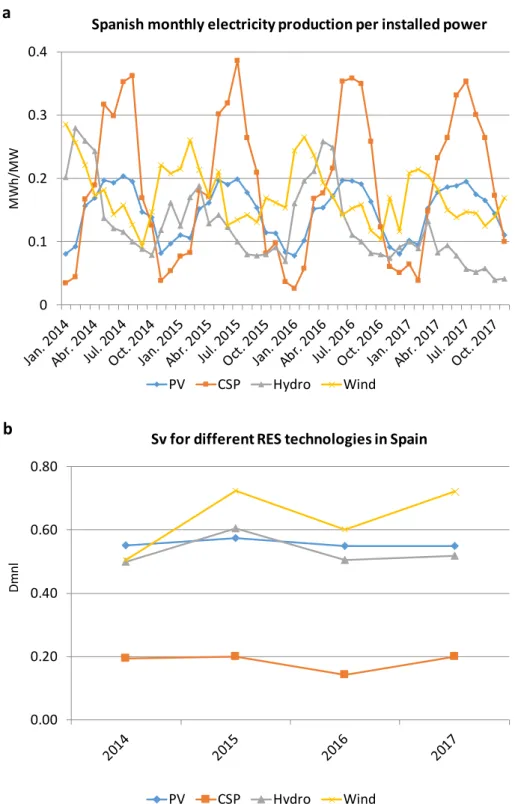
Figure 3: Seasonal variability of PV, CSP, Hydro and Wind for electricity production in Spain (2014-2017): (a) Monthly electricity production per installed power and (b) Sv. Own work from (REE, 2018).
Figure 3 shows that the monthly/seasonal (long-term) variability of CSP in Spain is much higher than for other RES (PV, wind, hydro). In the whole of Spain -which has 50 CSP plants and since 2013 is without new facilities- the Sv is <0.2, which is much lower than for photovoltaic (Sv ~ 0.55), wind (Sv = 0.5-0.72) and hydro (Sv=0.5-0.61), also with small capacity additions in the
0 0.1 0.2 0.3 0.4 MW h/ M W PV CSP Hydro Wind
Spanish monthly electricity production per installed power
0.00 0.20 0.40 0.60 0.80 Dmn l PV CSP Hydro Wind
Sv for different RES technologies in Spain
a
11
last few years (Figure 3). For the USA, from December 2016 to November 2017, Sv was 0.33 for CSP as against 0.69, 0.62 and 0.51 for Hydro, Wind and PV, respectively (data elaborated from EIA: https://www.eia.gov/electricity/monthly/). Sv data for the USA must be taken with precaution for PV and wind, because installed power continues to grow at an important pace. Table 3 collates the Sv for some individual CSP plants from the USA, Spain, UAE and India. We can roughly estimate Sv = 0.27 (the average of Spain and the USA, see Table 3) for plants in latitudes such as those of Spain and the USA, and Sv = 0.66 for plants in low latitudes (average of UEA and India). Solar Power Tower type plants seem to have a better Sv5 (although the CF is not improved), this and the better average radiation of the USA plants may be the reason that the USA average is better than the Spanish one. Given that, currently, more than 80% of the installed power belongs to Spain and the USA, the world average Sv at present is <0.3. Assigning 2/3 of the future potential of CSP in scenarios of high penetration of RES to areas of low latitude (high irradiance) and 1/3 to the rest, we would have an estimated Sv of around 0.5 for these scenarios.
Plant or system Sv
The USA 0.33
SEGS III-IX 0.03
Nevada Solar One 0.20
Mohave 0.12 Ivanpah 1 0.55 Ivanpah 2 0.49 Ivanpah 3 0.57 Genesis 0.20 Solana 0.37 Spain 0.20 Enerstar 0.21 Puerto Herrado 1,2 0.25 SHAMS (UAE) 0.77 Godawari (India) 0.55
Table 3. Calculated values of Sv. Sources: see references in text to build Table 2.
The electricity production variations in Spain comparing daily productions, instead of monthly, can be enormous. On the best days of the year (generally near the summer solstice, e.g. 22/06/2016, see Figure 4a), the average production can exceed 1,400MWe of instant power, reach the maximum between 10:30 and 20:30 and, with the help of storage and natural gas back-up, this is maintained for the rest of the day until 5:30 a.m. at 700MWe (1,000MW installed of the total of 2,300MW have storage of 7.5 hours or more); from 5:30 to 8:00, it decreases to 266MWe (here the gas necessarily intervenes, otherwise it would fall to zero). This pattern may occur for several days (no clouds over Spain).
On the other hand, the production of some several days on a row of December and January is practically zero (e.g. 25, 26, 27, 28 and 29 December 2017) (see Figure 4b). The average
12
production for those days (coinciding with the deep storm "Bruno" that entered Spain at that time) was about 18MWe (80 times lower than in the best days), with an equivalent CF = 0.0078. The storage of > 10 hours usually proposed to deal with hourly/daily variability, would increase the variability on the monthly/seasonal level, since on the cloudy days of winter the production would be practically null, while on the best days of summer, hourly storage would increase the average production (average CF increases with TES). In other words: hourly/daily storage exacerbates seasonal variability.
Figure 4: Instantaneous power generated by the 50 solar thermal plants in Spain on
12/06/2016 (a) and 25-29/12/2017 (b). On days 28 and 29 the production does not fall to zero during the night due to the hybridization of some plants with natural gas. Elaborated from the figures generated on (REE, 2018).
Section 6 includes a discussion of the implications of this seasonal variability for the CF of CSP plants in the context of scenarios of high RES penetration.
0
500
1000
1500
2000
2500
0
5
10
15
20
Electricity production of CSP in Spain (MWe)
Hour of the day (06/12/2016)
a
0 20 40 60 80 100 120 140 160 180 200 0,00 1,00 2,00 3,00 4,00 5,00Electricity production of CSP in Spain (MWe)
Days after 12/25/2017
b
13
5.
EROI
This section focuses on the estimation of EROI for CSP plants. Section 5.1 reviews the different EROI expressions used in the literature and justifies the expression applied in the analysis. Section 5.2 focuses on the estimation of Energy Used (EnU), taking as starting point previous works, which are complemented with literature review. Section 5.3 discusses which g factor (quality of electricity) to be applied, and finally section 5.4 presents the obtained results. To represent the implications for EROI of different levels of deployment of CSP, three scenarios are taken into account: scenario 1 considers current situation (reduced deployment near points of consumption and overcapacities and/or outside storage required to deal with intermittencies not considered), while Scenarios 2 and 3 refer to future scenarios with large scale deployment of CSP plants in hot deserts characterized by high irradiance, high winds, etc., (i.e., conditions similar to those of SHAMS 1 of UEA) (García-Olivares, 2016) . Both scenario 2 and 3 consider overcapacity requirements to deal with seasonal intermittency, the use of common materials and higher distribution losses than for scenario 1. While scenario 2 refers to regional distribution scenario 3 refers to international distribution (hence higher distribution losses for scenario 3 than for scenario 2) and less conservative embodied energies of some materials.
5.1. EROI expression
Until the present in the literature, there have been few studies specifically calculating the EROI of the CSP (Weißbach et al., 2013). However, there are several works that work with Life Cycle Assessment (LCA), in which the “Cumulated Energy Demand” (CED) or Cumulated Exergy Demand (CExD) is calculated and, from them, the Energy Payback Time (EPT or EPBT), which is the time measured in months or years in which the plant generates as much electrical energy as the electrical equivalent of the primary energy consumed.
CED is a term with origin in the LCA community. But there, CED is defined including all the primary energy harvested in the operation phase (in our case, the solar radiation over the CSP mirrors), that has no sense to calculate EPBT or EROI from CED and, therefore, is excluded of CED estimations from EPBT and EROI literature. To avoid confusion of the different “CEDs” being used in the literature, and given priority to the historical precedence to the CED defined by LCA community, we change the term to EnU (Energy Used) instead of CED when the purpose is to estimate EPBT or EROI.
According to different authors, Energy Payback Time is defined differently for CSP plants:
𝐸𝐸𝐸𝐸𝐸𝐸=𝐸𝐸𝐸𝐸𝐸𝐸𝐸𝐸𝐸𝐸𝐸𝐸𝐸𝐸𝐸𝐸
𝑔𝑔 − 𝐸𝐸𝐸𝐸𝐸𝐸𝐸𝐸
(eq. 1) (e.g. (Corona et al., 2014; Krishnamurthy and Banerjee, 2012; Lechón et al., 2008; Viebahn, 2013; Weißbach et al., 2013), where Enet is the yearly net electricity output (MJ/year), EnUc is the energy usedin its mineral extraction, manufacturing, construction and dismantling of the CSP plant (MJ), EnUo is the energy used associated with the operation and maintenance (MJ/yr), and g is a quality factor that compares the electricity generated with the primary energy consumed in the EnU. Note that the EnUs are given here in units of energy (MJ) and not in the ratios (MJ/KWh) that we will use in the next section that would be the EnUtot/Enet. Although exergy do not capture all the irreversibilities, if energy quality is taken into
14
consideration it will be better to use exergy and not primary energy (Weißbach et al., 2013), but there are few LCAs that use exergy (Ehtiwesh et al., 2016).
The other usual definition of the Energy Payback Time (e.g. (Burkhardt et al., 2011; Heath et al., 2011; Raugei et al., 2015) is:
𝐸𝐸𝐸𝐸𝐸𝐸𝐸𝐸 =𝐸𝐸𝐸𝐸𝐸𝐸𝐸𝐸𝐸𝐸𝐸𝐸𝐸𝐸𝐸𝐸𝐸𝐸𝐸𝐸/
𝑔𝑔
(eq. 2) where EnUtot is the sum of all primary energy (or exergy) supplied by sources across the LCA of the CSP plant and EnUtot = EnUc+EnUo·Life time.
Note that both definitions are different and give rise to different values of the Energy Payback Time.
Weisbach et al ., (Weißbach et al., 2013) proposes using the LCA methodology calculated by the EnU to estimate the EROI of different energy technologies. From the EPBT, the relationship would be established:
𝐸𝐸𝐸𝐸𝐸𝐸𝐸𝐸 = 𝐿𝐿𝐿𝐿𝐿𝐿𝐸𝐸𝐸𝐸𝐸𝐸𝐸𝐸𝐸𝐸𝐸𝐸𝐿𝐿𝑡𝑡𝐸𝐸=𝐿𝐿𝐿𝐿𝐿𝐿𝐸𝐸𝐸𝐸𝐸𝐸𝐸𝐸𝐸𝐸𝐸𝐸𝐸𝐸𝐸𝐸𝐿𝐿𝑡𝑡𝐸𝐸··𝐸𝐸𝐸𝐸𝐸𝐸𝐸𝐸𝑔𝑔
(eq. 3) In this paper, we propose not to use the EPT of (eq.1), as it can lead to physically impossible results. EPT or EPBT must be defined as positive (as well as the EROI). However, a system using more energy in operation and maintenance than the energy it provides (e.g. EnUo > Enet/g) is physically possible (although without much economic sense) but would give negative results according to eq. 1. Therefore, equation 1 should be discarded.
5.2. Energy Used by CSP system (EnUtot)
The literature usually estimates the energy requirements to build, maintain and dismantle a CSP plant and uses the so-called Cumulative Energy Demand (CED) (here EnU) and, more recently, the Cumulative Exergy Demand (CExD) (Ehtiwesh et al., 2016) (here ExU). For this calculation, a list of the minerals or materials necessary during the lifetime assigned to the plant is normally made and each of them is assigned the embodied energy intensity (MJ/kg), according to the Life Cycle Assessment (LCA) methodology. This energy is usually given in units related to the electrical production of the plant: MJ/KWh, which generates some confusion, because different authors assign different values to the electrical production of similar plants, which makes inter-comparability difficult. In addition, as we have analyzed (see section 3), all the reviewed studies use an overestimated CF, which therefore causes the overestimation of the electrical production that the plant will produce during its life-time. Table 4 shows the EnU values found in the literature (“EnUpublished”) as well as their correction, considering instead a CF = 0.25 (“EnUCED corrected”). When we use the term EnU without quotation marks we refer to cumulative energy demand in MJ or other energy dimensional unit. When we use the term “EnU”, we refer to MJ/KWh as is often used in the literature (although has no energy units).
Asdrubali et al., (2015) found a wide span in the values of “EnU” published in the literature, over 1 magnitude order of difference between the lower (0.2 MJ/kWh) and the higher (2.8 MJ/kWh) ranges; recent studies fit with this wide range (see Table 4).
15 Autor/technology “EnU” published “EnU” corrected (CF=0.25)
(Corona et al., 2016) hybrid Tower 1.337 2.19
(Burkhardt et al., 2011; Heath et al., 2011)
Parabolic 0.40-0.43 0.75-0.82
(Lechón et al., 2008) Parabolic-Tower 2.45-2.79 4.27-7.92
(Ehtiwesh et al., 2016) Parabolic 0.198 0.792
(Corona et al., 2014) Parabolic hybrid 1.15-3.20 1.47-4.81
(Asdrubali et al., 2015) (review range) 0.16-2.78
Table 4: “Energy Used” (“EnU”) of CSP plants in MJ/kWh found in the literature and its value if the CF were 0.25 instead of the one assumed in their theoretical works. The data of Asdrubali et al. (2015) are the extremes found in his review. The range for Corona et al. (2014) refers to different grades of hybridization with natural gas. The range of Burkhardt et al. 2011 refers to wet and dry technologies, respectively. The Lechón et al. (2008) data are for Parabolic and Tower, respectively. Note that, when corrected, the Tower “EnU” is much greater than Parabolic. Ehtiwesh et al. (2016) data refers to Exergy (destroyed useful energy), which results in 20% more than the same calculation performed with Energy. Thus, in the case of using exergy –which in our opinion is more consistent with the EROI calculations that weigh the quality of the energy source- and if the share were maintained, the rest of the values would be multiplied by approximately 1.2.
The re-estimation of “EnU”, taking into account real values for CF, increases the range to 0.8-7.9 MJ/kWh, i.e., an increase of 4x for the lower bound and almost 3 times for the upper bound of the range. Thus, the consideration of real values for CF is likely to affect the EPBT and EROI values previously published in the literature.
In this section, the EnU of a standard type of CSP plant is estimated for two cases (1) current plants (section 5.2.2.) and (2) plants in the context of high RES penetration scenarios (section 5.2.3). The applied methodology includes the review of previously published works, industry data and LCA databases. Previous works do not always take into account the same materials and energy costs associated with the LCA of the plant, but they can be combined, especially when some materials that others do take into account are missing in their calculations. Thus, Pihl et al., (2012) disaggregates mainly at the mineral level in detail and other authors disaggregate at the level of more elaborate materials (plastics, steels, etc.). In addition, as we will argue, some energy intensities of the materials (MJ/kg) that have been taken are different from the reality, or the reality that we would expect in a future of high penetration of renewable energy sources. That is why we have estimated the value of the EnU from the set of authors reflected in Table 4, for the material requirements per installed MW of a parabolic-type plant of 50 MW with TES, analogous to Andasol (Granada, Spain) or La Africana (also in Spain). Although Tower technology has a better Sv than Parabolic, we chose Parabolic with TES because it is the most proven technology at a commercial level. With a similar or better CF than other technologies, it is the most used for EnU and EROI estimations in the literature and probably has better EROI than other technologies (Lechón et al., (Lechón et al., 2008) using the same methodology, as both technologies show a slightly better EnU for Parabolic than for Tower. Since it considers a theoretical CF greater for the Tower, if the real CF is similar, this gives a much worse EnU for Tower (see Table 4)). The estimates are performed for three different scenarios, depending on the potential deployment level and geographical location of CSP over the next few decades.
Since aluminum is a much more abundant material than silver, thinking of scenarios of high solar penetration and trying to replace the more than foreseeable shortage of silver, there are proposals for scenarios of high penetration of RES with common materials (García-Olivares,
16
2016; García-Olivares et al., 2012). In this sense, ReflecTech, (2012) compares two types of parabolic mirrors, one classic (flat glass coated), based on silver (embodied energy of 35.24MJ/kg), with one based on recycled aluminium (embodied energy 24.29MJ/kg). However, in reality virgin ultrapure aluminium is used instead of Al recycled in the fabrication of mirrors given its higher purity which implies a better reflectivity (Vargel, 2004). Thus, in this work the embodied energy of the mirrors is re-calculated taking (ReflecTech, 2012) as a starting point but using instead data for virgin aluminium, obtaining 85.5MJ/kg if considering the value used by (Keough, 2011) data. The reflectivity is very dependent of purity: ultra-pure 99.99% aluminium has an 85% reflectivity versus 75% of aluminium with 99.6% purity (Vargel, 2004). The difference between the reflectivity of silver versus ultrapure aluminum is almost 12%, which would be directly reflected in the overall efficiency of the plants, while the embodied energies associated with the mirrors would be higher.
On the other hand, Ehtiwesh et al., (2016) consider 21.05MJ/kg for the energy intensity of the "molten salt" of the TES technology. However, if these salts are taken from the synthesis of ammonia and urea, which in turn come from natural gas, de Castro et al., ( 2013) reasoned that a strong scaling of this technology would exceed the reserves of the mines and that to synthesize it, more than 50MJ/kg would be required, since only the synthesis of urea and ammonia, from which these salts would be made, requires 40-50MJ/kg. Heath et al., (2011) considers that the associated emissions of CO2 (in one LCA) from the synthesis of salts versus those from mines would multiply these by a factor of almost 5; therefore, if we use the associated emissions as a proxy for embodied energy, the synthesis could require about 100MJ/kg.
Also, some authors who gave low “EnUs” in Table 4 (e.g. (Ehtiwesh et al., 2016)) do not take into account site preparation (removed lands, access roads, fences, waste ponds, retaining walls, etc.). For example, Turchi (2010), in an economic project, does take into account all these preparations, but takes a foot (0.3048m) of earth removed in the entire occupation of the plant. If we took 2Mm3 of land removed, as was done in La Africana of 50MW (La Africana, 2018) and 0.45MJ/Kg (from Hammond and Jones (2008)), it gives us a very conservative measure of energy for site preparation.
Heath et al., (2009) also consider materials that have little "weight", such as glass wool, refractory glass, calcium silicate and "small" machines, such as pumps, that would increase energy consumption by 2.5% over the total without taking into account this type of material. Reviewed studies do not correctly take into account the energy costs of the over-sizing of current lines, roads, fiberglass cabling, fences, natural gas conduction lines, etc., that leave the plant and connect them with the rest of the energy system of the country or region. These plants are located in deserts or semi-deserts, generally relatively close to towns and cities. However, as these areas are filled, the distances will be greater and far from the centers of consumption. So Kuenlin et al., (2013) calculate that the impact of the trans-regional lines, necessary for scenarios of high global penetration of renewables, can exceed 15% of the costs of the plant, which would surely be reflected in the embodied energies of these high and medium voltage lines. The Mohave project (Douglas et al., 2010) needs more than 150 kilometers of fiber optic cables to stabilize the electricity network, 32 monopoles of about 32 meters high, new paved roads, a fence of more than 2 meters along its 750 Ha of occupation, 2500m2 of waste treatment ponds with a base of 50cm of compacted silt surrounded by 60 cm high cement, 20 buildings for workers outside the solar field systems and the thermal power plant (control units, assembly factory of the modules, etc.). The 66 permanent workers of this 250MW plant have to travel several miles a day to go to the nearest towns where the necessary social infrastructures exist. Colonizing deserts requires greater energy effort than
17
other ecosystems (hence the density of population is always small). Turchi (2010) makes an economic study of the civil works, in addition to the industrial one, of a 103MW park (similar to that of Mohave), finding that operation and maintenance (O&M) have an economic cost of 30% of the construction, a number which could be used as a proxy to obtain the energy requirements of the O&M. If we consider the use of materials in the construction and maintenance phases, Pihl et al., (2012) gives some requirements in the maintenance phase of approximately 20% of associated embodied energy taking 25 years of plant life.
The data we have used for the materials embodied energies (MJ/Kg) comes, in general, from Hammond and Jones (2008), which uses the LCA criterion of Cradle to Gate (some of Cradle to site) for semi-fabricated components: sections, sheets, rods, etc., which go to the construction. To quote that article: "Highly fabricated and intricate items are beyond this report". Therefore, our methodology is probably conservative, compensating for the possible future improvement in the efficiency increase of the embodied energies.
5.2.1. Scenarios
We distinguish 3 scenarios for an Andasol or La Africana standard plant of 50MW: Scenario 1 represents the current situation (reduced deployment near points of consumption), while Scenarios 2 and 3 refer to future scenarios with large scale deployment of CSP plants in hot deserts characterized by high irradiance, high winds, etc., (i.e., conditions similar to those of SHAMS 1 of UEA) (García-Olivares, 2016). Scenarios 2 and 3 take into account the use of aluminum mirrors instead of silver (as in Scenario 1), given the potential scarcity of the latter in large-scale deployment scenarios of CSP (de Castro et al., 2013; Olivares, 2016; García-Olivares et al., 2012), as well as the loss of reflectivity of the aluminum mirrors relative to the silver mirrors and the damage suffered by mirrors due to severe winds in deserts. The three scenarios assume a life time of the plant of 25 years and a CF of 0.25. In particular:
- Scenario 1 considers molten salts from mines, silver mirrors and a regional distribution of electricity (embodied energy and losses of 5%) as the current plants with better CF. As mentioned above, the calculations will be conservative in terms of the total EnU requirements.
- Scenario 2 considers molten salts from the synthesis of urea with an embodied energy of 50MJ/kg, ultrapure virgin aluminum mirrors (85.5MJ/Kg) and the same regional distribution of losses in the electrical network as in Scenario 1.
- Scenario 3 considers molten salts from the synthesis of urea with an embodied energy of 100MJ/kg, an international distribution of electricity from deserts to points of high consumption, with embodied energy and losses of 15% of the total EnU found (García-Olivares, 2016; Trieb, 2006).
Section 5.2.2. reports the results obtained for the current CSP plants, while section 5.2.3. reports the results obtained considering the need for overcapacities in high RES penetration scenarios.
18
5.2.2. Current EnU of CSP plant
Table 5 reports the contribution by phase to the “EnU” for each scenario. Results are given in (MJ/kWh) per MW installed in order to compare our results with the literature (Table 4).
“EnU” (MJ/KWh) Scenario 1 Scenario 2 Scenario 3 Source
steels 0.37 0.37 0.37 (Ehtiwesh et al., 2016) concrete 0.02 0.02 0.02 (Ehtiwesh et al., 2016) plastics 0.10 0.10 0.10 (Montgomery, 2009) Syntetic oil 0.17 0.17 0.17 (Hammond and Jones, 2008; Pihl et al., 2012) molten salts 0.20 0.47 0.94 (Ehtiwesh et al., 2016) corrected Ag based mirror 0.08 0.00 0.00 (Ehtiwesh et al., 2016; ReflecTech, 2012) Al based mirror 0.00 0.26 0.26 (Keough, 2011; ReflecTech, 2012)
site preparation 0.49 0.49 0.49 (La Africana, 2018)
other material and
machineries 0.03 0.03 0.03 (Heath et al., 2009)
broken mirrors 0.00 0.03 0.07 (Radan, 2016)
water (distilled 0.2MJ/kg) 0.13 0.13 0.13
(Hammond and Jones, 2008, p. 20; Kuenlin et al., 2013; Turchi, 2010)
Cu, Mg and other metals 0.02 0.02 0.02
(Hammond and Jones, 2008; Pihl et al., 2012) rock 0.02 0.02 0.02 (Hammond and Jones, 2008; Pihl et al., 2012) Operation phase 0.19 0.19 0.19 (Hammond and Jones, 2008; Pihl et al., 2012)
Dismantling and disposal 0.05 0.06 0.07
(Burkhardt et al., 2011; Heath et al., 2011)
Dry cooled performance 0.14 0.18 0.22 (Heath et al., 2011)
Al mirror reflectivity loss 0.00 0.36 0.43
(García-Olivares 2016)
Grid needs and losses 0.18 0.18 0.54
(García-Olivares, 2016; Trieb, 2006)
“EnU”tot 2.18 3.07 4.06
Table 5: Energy Used (EnU) for materials
The “EnU” levels obtained for scenarios 1 and 2 are in the high bound of the literature review (Table 4) and over the high bound for scenario 3. The latter is consistent with the fact that scenario 3 is assessing CSP in conditions which have not been studied in other studies.
19
In relation to the contribution to the “EnU” for each phase/material processing varies depending on the scenario (see table 5 and the detailed results in Appendix A):
For both scenarios 1 and 2, site preparation, steels and molten salts account for ~45-50% of the “EnU”, followed by the energy requirements associated to the operation phase, grid needs and losses, and in the case of scenario 2, the Al based mirrors and Al mirror reflectivity loss. For scenario 3, molten salts, grid necessities and site preparation represent ~50% of the “EnU”, followed by Al mirror reflectivity loss, steels, Al based mirror and Dry cooled performance (together accounting for ~80% of the total “EnU”).
The issues associated with intermittency, need of back up etc., and the associated embodied energies, are not considered in Table 5. These additional requirements could be currently low in most countries, given the relatively low penetration of intermittent RES, although relatively to the own intermittent RES penetration this costs could be important (e.g. intermittent RES impose some adaptation of the grid system, therefore, some investment and some energy cost). In any case, in high RES scenarios, it is necessary to take them into consideration. The next section is dedicated to estimating the EnU under these conditions.
5.2.3. EuN of CSP plants in high RES penetration scenarios
Apart from hydro pumping storage (PHS), storage systems to compensate for the seasonal variations are not yet available and alternative technologies of large-scale storage are still in the R&D phase (Wagner, 2014). Thus, apart from flexible demand management, overcapacity is probably the best strategy to deal with seasonal and annual variation. As mentioned in section 4, the Sv can be used to estimate the required overcapacity to deal with seasonal variability in systems with high penetration of solar technologies. The criterion of Capellán-Pérez et al., (Capellán-Capellán-Pérez et al., 2017b) to ensure that the month of lowest irradiance meets the average annual demand for electricity required, allows the difference between the irradiance of winter against that of summer to be taken into account. In accordance with this criteria, the inverse of Sv is the overcapacity (f) to be added to a mix with strong variable RES penetration (see eq. 3 in Capellán-Pérez et al., (Capellán-Pérez et al., 2017b)), then the CF at the plant level is:
𝐶𝐶𝐶𝐶 =12𝑃𝑃𝑃𝑃𝑃𝑃·𝐴𝐴𝐴𝐴𝐴𝐴 (eq. 4)
Ave being the monthly average power production and Pow the gross nominal power of the plant or present system. If overcapacity is required for seasonal variation, the effective CF
(CF,eff) at the system level with strong RES penetration will be:
𝐶𝐶𝐶𝐶,𝐸𝐸𝐿𝐿𝐿𝐿=12𝑃𝑃𝑃𝑃𝑃𝑃·𝐴𝐴𝐴𝐴𝐴𝐴·𝑓𝑓 =𝐶𝐶𝐶𝐶·𝑆𝑆𝑆𝑆=12·𝑃𝑃𝑃𝑃𝑃𝑃𝐿𝐿𝑃𝑃𝑃𝑃𝐴𝐴𝐿𝐿𝐿𝐿 (eq. 5)
Where Lowest is the power production in the lowest monthly production of an average annual electricity production.
In a future with a high penetration mix of RES with strong penetration of seasonal variables, RES, CF,eff will be an underestimation of the effective CF of the CSP system, if we consider that no other intermittencies are taken into account (see below). This could be an overestimation only if the ratio of strong seasonal variables RES over non seasonal variables is low (Capellán-Pérez et al., 2017b). However, all analyzed high penetration RES scenarios from Table 1, and other assessed high RES penetration scenarios, have a very high use of wind and solar relative to biomass and geothermal power (with an Sv that could be close to one, if so desired, because monthly production does not depend on geographical latitude or climatology).
20
Thus, Lenzen et al., (2016) goes from a CF = 0.6 for a CSP plant to a CF = 0.35 for the CSP system when the electrical system is 100% RES. Delucchi and Jacobson ( 2011) give an initial CF of 0.31 for plants, but when they build their 100% RES model in Jacobson and Delucchi (2011), they reach a final CF = 0.18 for the CSP system. In both studies, the CF is reduced to 60% of its initial value. If we take equation 5 to compare, these values would be equivalent to Sv = 0.6. To estimate them in high RES penetration scenarios, other methodologies have been considered for the calculations of the embodied energy of the materials used for construction, operation and dismantling (see Table 6).
“EnU” (MJ/KWh) Scenario 1 Scenario 2 Scenario 3 Materials in construction, operation,
dismantling and disposal, with grids 2.18 3.07 4.06
Overcapacity for intermittence, back up, etc. (Lenzen and Deluchi models)
1.45 2.05 2.71
Overcapacity for seasonal intermittence (this work)
2.18 3.07 4.06
“EnU”tot (Lenzen/Deluchi models) 3.63 5.12 6.77
“EnU”tot (this work) 4.36 6.14 8.12
Table 6: Total “EnU” (Energy Used) estimated in tree scenarios for materials and overcapacity for two methodologies.
According to our calculations of CF, eff = Sv · CF ~ 0.5 · CF (see eq. 6 and section 4), which would require twice the infrastructure to give the same CF, eff without the need for overcapacity. Then the EnUtot would be multiplied by 2. In the same way, taking the CF reduction factor of the Lenzen et al., (2016) and Jacobson-Delucchi models, the EnUtot would increase by 67%.
5.3. The g factor (average efficiency in the transformation of primary energy to
electricity and the quality of the energy)
Different authors use different criteria for the value of g. Thus, most authors take g as the average efficiency in the transformation of primary energy to electricity and this is usually taken as that of the specific country where the plant is studied. This efficiency depends on the electricity mix of each country, as well as the evolution over time of the efficiency of different electricity transforming plants (taking a past or present value tends to give lower values of the EPBT than if values of the future are taken, where a relative increase in electricity as a final energy use, or an increase in the efficiency of thermal plants, would give values greater than g at present). We call this criteria, "primary energy replacement".
Given that there is no term of quality in the classic definition of the EROI and given that, to assure more consistency, the LCA should use exergy and not primary energy, Weißbach et al., (Weißbach et al., 2013) uses the value 1 for the g factor. We call this criteria, "direct electricity output". Thus, we define an EROIg=1 following the ”direct electricity output” criteria (Weißbach et al., 2013), taking the destroyed exergy of equal quality as electricity (g = 1). On the other hand, we call it EROIg=0.456 when following Raugei et al., (2015) reasoning when they criticize Weisbach's methodology and consider that the EnU must be modified by a factor: “the average ‘life cycle efficiency’ of the grid” (“primary energy replacement” criteria). With data from 2013 worldwide, we find that the electricity production is 2,232 Mtoe for primary electricity of 5,111Mtoe; then the factor on a global scale is 0.456 (IEA, 2018) (also available at https://www.iea.org/Sankey/). Therefore, g = 0.456 and EROIg=1 = EROIg=0.456/0.456
21
However, Prieto and Hall (2013) argue that, although electricity actually has more quality as an energy source than others, on a global scale, only ¼ of the final energy needs are covered by electricity and the rest by other forms (heat, mechanical ...), and it is not obvious that they have that factor g but, in the case of heat, it could be greater than 1. For the specific case of CSP plants, we can suspect that this is effectively the case when they usually hybridize with natural gas, probably for reasons of economic efficiency, but in this case indicates that, for this part of the consumption, the factor of "quality" g would be greater than 1, since real plants are using natural gas to preheat the thermal fluid instead of electricity, despite the fact that the plant produces electricity and could only consume electricity (not strictly requiring to be connected to a natural gas pipeline).
Here, we propose and finally use a new criterion following the arguments of Prieto and Hall (2013), that we will call “final to primary energy” criteria. We call it EROIg=0.687, and that is to take g by directly comparing the final energy consumed (discounting the non-energy uses that are mixed in the statistics) with the primary energy (also discounting the proportion that does not go to energy) provided by the IEA in its Sankey diagram for the World. The result is a g = 0.687.
This also agrees with general global studies which aim to evaluate the substitution of the current energy system towards a renewable one with a total electrification of the system: Thus, García-Olivares et al., (García-Olivares et al., 2012) conclude that we would need almost 70% of the primary energy that we consume today in an electric form to provide the same services.
Therefore, in this work, we consider EROI = EROIg=0,687 = EROIg=1/0.687.
An alternative, beyond the scope of this work but consistent with our criteria here exposed, is to consider g dynamically, given that the average efficiency in the transformation of primary energy to electricity will change (increase) during the transition to renewables. However, this requires a more complex modeling, for example, the approach taken to build the MEDEAS models (Capellán-Pérez et al., 2017a).
For sensitivity purposes and because it is an ongoing debate, in Appendix B some results are re-elaborated assuming different values of g (g=1 and g=0.456).
5.4. Estimation of EROI
Hall et al., (2014) propose different calculations for the EROI, distinguishing between EROIst (standard), EROIpou (point of use) and EROIext (extended). The latter extends the boundaries of the calculations and is more coherent if the aim is to compare complete systems and not particular plants. Since complete systems usually lack data, or we must hypothesize what the complete system would look like in future energy mixes, the EROIext usually starts from indirect estimates based on associated economic costs and then, through some energy intensity function (on a national or global scale), calculates the complete energy costs that do not usually appear in the LCA (e.g. any necessary economic transaction, such as the paid work of the project engineer, requires an indirect energy consumption associated with the energy intensity of said economic transaction). In the extended calculations of the EROI, estimates associated with support infrastructures that a future energy mix based mainly on renewables would require (e.g. external storage infrastructures or overcapacities) and that today are not necessary may also be included. Here, we use this last criterion, which in reality would not generate an EROIext, but a conservative estimation of the EROIpou. Therefore, from the
22
EROIext approach, the presented calculations would be very conservative, since EROIst> EROIpou> EROIext.
A total of 11 studies have been reviewed that report analyses for 15 CSP power plants of different typologies and functioning under different conditions (Burkhardt et al., 2011; Corona et al., 2016, 2014; Ehtiwesh et al., 2016; García-Olivares, 2016; Heath et al., 2011; IEA and IRENA, 2013; Krishnamurthy and Banerjee, 2012; Lechón et al., 2008; Montgomery, 2009; Viebahn, 2013; Weißbach et al., 2013). Table 7 shows the reported EROIst in the papers (“Reported EROI” column), if the papers do not report the EROIst, the column shows the estimates of EROIst that we can deduct based on the reported data. The “Standarized EROIst” column shows our re-estimation, if possible considering the real values for CF found in section 3 and considering g=0.687. Reported EROI Standardized EROIst (CF=0.25 & g=0.687) Burkhardt et al., 2011 27.7-30 -a
Corona et al., 2014 (hybrid range) 14.1-17.5 1.47-3.41
Ehtiwesh et al., 2016 20.2 7.74
Heath et al., 2011 30 6.97
IEA and IRENA, 2013 60
Krishnamurthy and Banerjee, 2012 7.44-12.2
Lechón et al., 2008 (Tower) 24.6 1.88
Lechón et al., 2008 (Parabolic) 24 2.14
Weißbach et al., 2013(Parabolic) 21 ≈1
(if buffered) (EROIpou) 9.6
Viebahn, 2013 (range) 10.9-67.6 5.02
Montgomery, 2009 22
García-Olivares, 2016 18
Table 7: This table gives the calculation of the EROI that the authors give directly or can be deduced from their estimates of other parameters. Some authors give several technologies or hypotheses (first column). The second column repeats the calculations using equation 4 where appropriate, a CF = 0.25 if the technology has storage and CF = 0.2 without storage. The factor g here is taken as 0.687. a Empty cells refer to cases where it was not possible to recalculate the EROI.
23
From the table EnUtot calculated in this study, and taking the value g = 0.687, we would obtain the following EROI levels for each scenario (Table 8):
EROI Scenario 1 present system scenario 2 future system Scenario 3 future system EROIst (Materials in construction,
operation, dismantling and disposal
including grids) 2.4 1.7 1.3
EROIpou (present CSP) <2.4 - -
EROIpou (system, high penetration
Lenzen and Deluchi models) 1.4a 1.0 0.8 EROIpou (system, high penetration
this work) 1.2a 0.85 0.65
Table 8: Conservative (reality probably lower) estimated values of the EROIst (first row) and the EROIpou (second, third and four rows) for the CSP according to three scenarios and different methodologies, taking the quality factor of electricity g = 0.687. The EROIpou for the present system is not estimated (see text). a Supposing the scenario 1 (“present system”: Ag based mirrors, mined salts, CSP installations near consumer centers) but with the over cost of high penetration of CSP to deal with intermittences, see text for details of scenarios.
In relation to EROIst, the obtained values are 2.4:1 for scenario 1, 1.7:1 for scenario 2 and 1.3:1 for scenario 3. We only estimate the EROIpou for high penetration escenarios; The EROIpou for the present system is not estimated, it will add relatively to the EROIst the embodied energy that the energy system demand to deal with the intermittencies that CSP impose over the system grids (see figure 4). RES penetration in Spain and USA is concomitant with the lowering of CF of the quick response of new natural gas power installations, therefore, the electric grid system is adapting with energetic cost to the present penetration. But, because the RES variables are not the main sources of electricity, it is very difficult to estimate what it is the over cost attributable to CSP (for instance the energy cost of PHS) against the rest of energy sources (most fossil and nuclear fuels). From NREL 2012 model (for USA) one can deduct that the cost tend to increase with the penetration of RES variables in relative terms (the % of over cost increase with the % of RES penetration) and that the present cost (with less than 20% of RES variables in the electricity mix) of storage and overcapacities (e.g. natural gas power plants) atributable to RES variables are not null. For both methodologies considered
(Lenzen/Delucchi and this work), only Scenario 16 would (barely) have an EROIpou>1:1, while both Scenarios 2 and 3 would fall into EROIpou<1:1. EROIpou take into account storage needs at hourly intermittence level (by TES technology) and the overcapacity needed to deal with seasonal intermittence, but not the storage needed for day/week intermittence (e.g. pumped hydro storage for several days as reflected in Figure 4b), therefore it is probably conservative. Tables B1 and B2 in Appendix B re-estimate the obtained values in Tables 7 and 8 respectively considering alternative values for the g factor in the literature (g=1 and g=0.456). The obtained EROI levels following g=1 criteria are lower. The recalculation of EROI from other studies of the literature applying g=1 criteria provide EROI values below the ratio 3:1 (Table B1); while the EROIst obtained in Scenario 1 is already as low as 1.65:1 (Table B2). On the other hand, following g=0.456 criteria, the EROI levels are slightly improved. The recalculation of EROI from other studies of the literature with g=0.456 provide EROI values which provide a wide range of 2.2-11.66:1 (Table B1). In relation to the EROIst obtained in Scenarios 1, 2 and 3, the value in
6 Although scenario 1 refers to present conditions, we suposse here that this present conditions could
be extrapolated to high penetration of CSP in the electricity mix, this result in very conservative estimations of EROI (optimistic)
24
Scenario 1 reaches 3.62:1, while for EROIpou of the system in Scenario 1 decreases until 2:1 (Table B2). Hence, the consideration of different values for the g factor does not modify the main conclusions of the analysis presented in this paper.
6. Discussion and conclusions
As mentioned in the introduction, analyses proposing a high share of CSP in future 100% RES scenarios rely on the ability of this technology, through storage and/or hybridization, to partially avoid the problems associated with the hourly/daily (short-term) variability of other renewable variable sources, such as wind or PV (e.g. (Delucchi and Jacobson, 2011; García-Olivares, 2016; Greenpeace et al., 2015; Jacobson et al, 2016; Jacobson and Delucchi, 2011;
WWF, 2011)). However, this advantage seems to be more than offset by the overall
performance of real CSP plants. In fact, the obtained results from CSP plants in operation, using publicly available data from 4 countries (Spain, the USA, India and UAE) show that the actual performance of CSP plants is shown to be significantly worse than projected by constructors and considered by the scientific literature in the theoretical studies: capacity factors in the same order as wind and PV, low EROI, intensive use of materials –some scarce- and significant seasonal intermittence. The consideration of these factors would likely modify the conclusions of the analyses reviewed in Table 1.
In particular, real data shows that the capacity factor attributable to the solar energy of the CSP plants is currently in the range of 0.15-0.3, representing a strong reduction in relation to the range of usually expected values by the industry (0.2-0.5) and the common values used in the academic literature (0.25-0.75) (for the currently most studied technology, Parabolic with TES, the theoretical CF in the literature is around twice the real performance). This bias may seem especially paradoxical in the case of the scientific literature; given that there has been publicly available data for many power plants for years (e.g., SEGS plants in the USA have been operating since the end of the 1980s). CF is a key parameter that critically affects the life-cycle analyses that estimate the energy and material requirements (such as the energy payback time (EPBT) and EROI) as well as the environmental impacts and economic costs.
Depending on the technology, the seasonal variability can be even worse than for wind or PV, as has been shown for the case of Spain and the USA, where the output can also be zero for many days in winter. Given that storage systems on the required scale to compensate for the seasonal variations are not yet available and alternative technologies of large-scale storage are still in the R&D phase (Wagner, 2014), the solution would require a combination of overcapacities and flexible demand.
On the other hand, low latitude locations with high irradiances, such as hot deserts, are more difficult to colonize (wind, dust/sand, extreme temperatures, water scarcity, etc.). Although the seasonal variability in the studied plants in India and UEA improves in relation to those in the USA and Spain, the fluctuations are still of the same order of magnitude as for other RES, such as wind and PV. In desert areas, dust storms can also cover large regions during several days (e.g. over the Sahara and the Arabian Peninsula in March 2010 (NASA EO, 2010)). These dust storms explain why the analyzed CSP plant in UEA SHAMS 1 has a lower annual average DNI than the CSP plants from the USA (located at higher latitudes). In regions affected by the monsoon, such as India, the observed Sv in the Godawari CSP plant is 0.55, which is lower than the expected from the variation in total irradiance at country level (Sv for India of 0.76 (Capellán-Pérez et al., 2017b)).