Modular and efficient pre-processing of single-cell RNA-seq
Páll Melsted
1,*, A. Sina Booeshaghi
2,*, Fan Gao
3
, Eduardo Beltrame
3, Lambda Lu
3,
Kristján Eldjárn Hjorleifsson
4, Jase Gehring
3and Lior Pachter
3,41. Faculty of Industrial Engineering, Mechanical Engineering and Computer Science, University of Iceland, Reykjavik, Iceland
2. Department of Mechanical Engineering, California Institute of Technology, Pasadena, California
3. Division of Biology and Biological Engineering, California Institute of Technology, Pasadena, California
4. Department of Computing and Mathematical Sciences, California Institute of Technology, Pasadena, California
Address correspondence to [email protected] * Authors contributed equally
Abstract
Analysis of single-cell RNA-seq data begins with the pre-processing of reads to generate count matrices. We investigate algorithm choices for the challenges of pre-processing, and describe a workflow that balances efficiency and accuracy. Our workflow is based on the kallisto and bustools programs, and is near-optimal in speed and memory. The workflow is modular, and we demonstrate its flexibility by showing how it can be used for RNA velocity analyses.
Introduction
The quantification of transcript or gene abundances in individual cells from a single-cell RNA-seq (scRNA-seq) experiment is a task referred to as pre-processing of the data1. The
pre-processing steps for scRNA-seq bear some resemblance to those used for bulk RNA-seq2,
and are in principle straightforward: cDNA reads originating from transcripts must be partitioned into groups according to cells of origin, aligned to reference genomes or transcriptomes to determine molecules of origin, and reads originating from PCR-duplicated molecules must be “collapsed” so they are counted only once during quantification. The collapsing step can be facilitated with unique molecular identifiers (UMIs), which are sequences that serve as barcodes for molecules3. The challenges in pre-processing single-cell RNA-seq lie in the tradeoffs that
must be considered in determining choices for how, and in which order, to execute the various steps. For example, in droplet-based scRNA-seq protocols, collapsing UMIs to account for PCR duplication can be performed naïvely by associating all reads that align to the same gene, with the same UMI, to a single molecule4. This computationally efficient procedure is based on an
assumption that all reads with identical UMIs that align to the same gene arise via PCR duplication of a single molecule. Alternatively, this assumption can be relaxed, resulting in a problem formulation that is NP-complete, i.e. computationally intractable to solve optimally5.
Another challenge in scRNA-seq pre-processing is the amount of data that must be processed. A single cell experiment can generate 106 - 1010 reads from 103 - 106 cells6. This is leading to
bottlenecks in analysis: for example, the current standard program for processing 10x Genomics Chromium scRNA-seq, the Cell Ranger software7, requires approximately 22 hours to process
784M reads5. For this reason, a number of new, faster workflows for scRNA-seq pre-processing
based on pseudoalignment8 have recently been developed 5,9. However, despite improvements
in running time, current workflows have memory requirements that increase with data size5, a
situation that is untenable given the pace of improvement in technology and the corresponding increase in data.
In recent work we introduced a new format for single-cell RNA-seq data that makes possible the development of efficient workflows by virtue of decoupling the computationally demanding step of associating reads to transcripts and genes (alignment), from the other steps required for scRNA-seq pre-processing10. The new format, called BUS (Barcode, UMI, Set), can be
produced by pseudoalignment, and rapidly manipulated by a suite of tools called BUStools. To illustrate the utility, efficiency, and flexibility of this approach for scRNA-seq pre-processing, we describe a Chromium pre-processing workflow based on reasoned choices for the key
pre-processing steps. While we focus on Chromium, our workflow is general and can be used with other technologies. We show that our pre-processing workflow is much faster and more memory efficient than existing methods, and we demonstrate the power of modular processing with the BUS format by developing a fast RNA velocity analysis workflow11. We also validate the
design decisions underlying the Cell Ranger workflow. Our benchmarking and testing is comprehensive, comprising analysis of almost two dozen datasets and greatly eclipsing the scale of testing that has been performed for current workflows.
Results
In designing a scRNA-seq pre-processing workflow, we began by investigating each required step: correction of barcodes, collapsing of UMIs, and assignment of reads to genes. To achieve single-cell resolution, the Chromium technology produces barcode sequences that are used to associate cDNA reads with cells, and we began by considering the efficiency-accuracy tradeoffs involved in grouping reads with the same, or similar, barcodes to define the contents of
individual cells. The Chromium barcodes arise from a “whitelist”, a set of pre-defined sequences that are included with the Cell Ranger software. Grouping reads according to barcode is
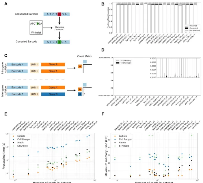
therefore straightforward, except for the fact that barcodes may contain sequencing errors. The Cell Ranger workflow corrects all barcodes that are one base-pair change away (Hamming distance 1) from barcodes in the whitelist. An examination of a benchmark panel of 20 datasets revealed that this error correction approach can be expected to rescue, on average, 0.8% of the reads in an experiment (Figure 1a,b), a calculation based on an inferred error rate per base for each dataset (Methods, Supplementary Table 1). Thus, correction of barcodes Hamming distance 2 away from whitelist barcodes would rescue, on average, a negligible number (0.0038%) of reads (Methods). We therefore implemented a Hamming distance 1 correction method in our workflow via the bustools correct command.
Next, in considering how to collapse UMIs, we first investigated the extent to which “collisions” occur, i.e. cases where the same UMI occurs in reads originating from two different molecules. While inter-gene collisions can be directly measured, intra-gene collisions cannot be
distinguished from PCR duplicates. To estimate the intra-gene collision rate we first calculated, for each cell in the benchmark panel, the effective number of UMIs in each of the associated droplets (Supplementary Figure 1, Supplementary Note). This estimate, along with the number of inter-gene collisions and distinct UMIs observed, allowed us to estimate the extent of
intra-gene collision, and therefore the count loss due to naïve collapsing of UMIs by gene (Methods, Supplementary Note). We found that the average percentage of lost counts per gene per cell due to naïve collapsing was less than 0.003% for v2 chemistry and 0.000048% for v3 chemistry (Figure 1c,d). Thus, we decided to apply naïve collapsing as it is computationally efficient and effective based on empirical evidence. This was implemented in the bustools count command. Notably, the recently published Alevin collapsing algorithm5 will overestimate
gene counts because reads with the same UMI pseudoaligned to the same gene are very likely to be from the same molecule even if they pseudoalign to distinct transcripts. In fact, our
analysis suggests such situations result from missing or incorrect annotation12 rather than from
collisions where two distinct molecules are labeled with the same UMI.
One implication of the UMI collapsing analysis is that UMI error correction is possible because UMIs with only one base-pair change away from an abundant UMI are likely to have resulted from sequencing error. To examine the benefit of such a correction we computed the expected number of UMIs that would be corrected with Hamming distance 1 correction, and found that for 10bp and 12bp UMIs only 0.5% and 0.6% of reads would be recovered, respectively, at the error rates observed in published datasets (Methods, Supplementary Figure 2). Moreover, such error correction would require identification of abundant UMIs in lieu of a whitelist, adding time and complexity to the workflow. While we believe such error correction may be warranted in the case of longer UMIs (Supplementary Figure 2), we did not include it in our workflow.
In most scRNA-seq pre-processing workflows, assignment of cDNAs to genes utilizes genome alignment4,13,14 . Since detailed base-pair alignment is not necessary to generate a count matrix,
pseudoalignment to a reference transcriptome8 suffices. Moreover, pseudoalignment has been
shown to be highly concordant with alignment for the purposes of quantification in bulk
RNA-seq15. To test this hypothesis we compared counts obtained by pseudoalignment using the
kallisto program8 with counts produced via Cell Ranger which is based on the STAR aligner16.
Analysis of an Arabidopsis thaliania scRNA-seq dataset (Figure 2), confirms that there is a high correlation between pseudoalignment and alignment based counting, however in one dataset (pbmc10k_v3, Supplementary Figure 3.19) we found that pseudoalignment produced more counts than alignment. Specifically, in the FGF23 (ENSG00000118972) gene, Cell Ranger had many fewer counts than kallisto. We hypothesized that the reason for this discrepancy was the presence of reads from unspliced transcripts crossing splice junction boundaries, and therefore being erroneously pseudoaligned to the transcriptome. To test this we created a modified index that included a 90 base-pair overlap into the exon and the intron (one base-pair less than the length of the reads) to capture such reads and confirmed that it resolved the discrepancy (Supplementary Figure 4). We observed this problem to be rare and therefore did not deem it to be essential in a standard processing workflow. It may be that consideration of such reads will be crucial for nuclear scRNA-seq analyses17, when the abundance of such intronic junction
reads will be problematic for naïve pseudoalignment.
Thus, our workflow consists of pseudoalignment of reads to a reference transcriptome to generate a BUS file, and subsequent processing to correct barcode errors and produce a count matrix (Supplementary Figure 5). To ensure that memory usage is constant in the number of
reads, the BUS files are sorted by barcode prior to counting using the bustools sort command. While this workflow is very similar to that of Cell Ranger, it is not identical. Since Cell Ranger is widely used, we investigated the extent to which the Cell Ranger results are concordant with our workflow. We processed 20 datasets (Supplementary Table 1), chosen to contain a range of reads depths (from 8,860,361 to 721,180,737 reads per sample and 2,243 to 201,952 reads per cell) and to represent scRNA-seq from a range of tissues and species (Arabidopsis thaliania18,
Caenorhabditis elegans19, Danio rerio20, Drosophila melanogaster 21, Homo sapiens22,23, Mus
musculus24–28, Rattus norvegicus28). We found a high degree of concordance with respect to
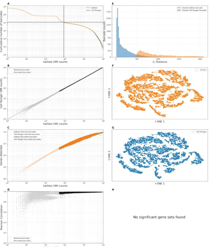
quality control metrics (Figure 2a—h, Supplementary Figure 3). Crucially, in all datasets, in a joint analysis of kallisto and Cell Ranger counts, the closest cell to a kallisto cell was its associated Cell Ranger cell, i.e. the Cell Ranger cell with the same barcode sequence. Furthermore, correlations between gene counts in individual cells that passed Cell Ranger filtering criteria were almost always above 90%, and frequently as high as 99%.
To assess the extent to which differences between Cell Ranger and kallisto affect biological inferences, we also compared Cell Ranger to kallisto in a variety of typical downstream analyses on the 10x Genomics E18 mouse 10k brain cells dataset. The Cell Ranger analysis produces structures similar to that of kallisto when projected to the first two principal components (PCs) and to two dimensions of tSNE (Supplementary Figure 6.1). The results of Leiden clustering29
are similar regardless of pre-processing workflow, though while most clusters can be uniquely matched between Cell Ranger and kallisto, there are a few cases of cluster merging and splitting (Supplementary Figure 6.2). We performed differential expression (DE) analysis to identify marker genes of the clusters, and then performed gene set enrichment analysis (GSEA) on the marker genes for cell type annotation (Supplementary Figure 6.3). The marker genes and their corresponding gene sets were highly correlated between the workflows. In both Cell Ranger and kallisto results, most clusters seem neuronal, and the clusters for erythrocytes (cluster 16 in both), endothelial cells (cluster 21 in kallisto, cluster 19 in Cell Ranger), and immune cells (clusters 20 and 22 in kallisto cluster 17 in Cell Ranger) can be clearly identified based on marker genes (Supplementary Figure 6.3). Correlation between the same barcodes in kallisto and Cell Ranger with the top cluster marker genes is very high, with both the Pearson and Spearman correlation coefficient above 0.9 for the vast majority of cells (Supplementary Figure 6.4). Pseudotime inference with Cell Ranger and kallisto resulted in concordant
trajectories from neuronal precursor cells to two populations of neurons, with the same trajectory topology and similar pseudotime values along the trajectory (Supplementary Figure 6.5). In a separate mixed species dataset, the number and proportion of UMIs from human and mouse cells are similar between Cell Ranger and kallisto (Supplementary Figure 7). Overall, these results suggest that the Cell Ranger workflow produces results consistent with our method, not only at the level of dataset summary statistics, but also in downstream analyses.
The modularity of our approach makes possible the rapid implementation of alternative workflows. To illustrate this we developed an RNA velocity workflow. By including intron sequences in the index for pseudoalignment we were able to identify reads originating from unspliced transcripts, and, using the bustools capture command, efficiently created the spliced and unspliced matrices needed for RNA velocity. Our RNA velocity workflow, which is 13 times faster than velocyto11, is suitable for analysis of large datasets that were previously challenging
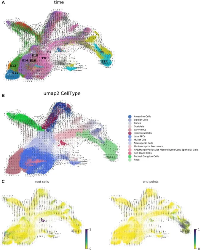
to pre-process. To illustrate this we computed RNA velocity vectors for recently published data from the developing mouse retina30 consisting 113,917 cells (Figure 3). We found that six
Rbpms, Rlbp1) displayed patterns consistent with the RNA velocity vectors, and with the pseudotime analysis of Clark et al.31 (Supplementary Figure 8). The velocity analysis reveals
new information, namely it identifies developmental states when velocity is changing
(Supplementary Figure 8 middle column). We verified the fidelity of our workflow by computing RNA velocity vectors on a dataset from La Manno et al. 201811 and comparing our results to
those of the paper (Methods, Supplementary Figure 9). We were able to identify many more counts in the unspliced matrix (Supplementary Figure 10), and our resultant velocity figure was concordant with that of La Manno et al. 201811.
Discussion
Our scRNA-seq workflow is up to 51 times faster than Cell Ranger and up to 4.75 times faster than Alevin. It is also up to 3.5 times faster than STARsolo: a recent version of the STAR aligner adapted for scRNA-seq (Figure 1e, Supplementary Table 2). Importantly, unlike these other programs, our workflow requires a small fixed amount of constant memory that is independent of the number of reads being pre-processed (Figure 1f). It is therefore suitable for low-cost and environmentally conscious cloud computing. Moreover, the workflow is scalable and can in principle be used for pre-processing arbitrary numbers of reads. In benchmarks on the panel described in this paper, kallisto’s running time was comparable to that of the word count (wc) command applied to the FASTQ files, suggesting that kallisto is near-optimal in efficiency (Supplementary Figure 11). Our speed and constant memory requirements make RNA velocity tractable for datasets of any size for the first time.
Our UMI collapsing analysis suggests that UMI sequences can be short; even just 5 base-pairs of sequence suffice for identifying molecules thanks to the cell barcode and gene identification for each read serving as auxiliary barcodes (Supplementary Figure 12). Furthermore, the fact that identical UMIs associated with distinct reads from the same gene are almost certainly reads from the same molecule, makes it possible, in principle, to design efficient assignment
algorithms for multi-mapping reads. Reads could be assigned with an expectation-maximization algorithm which is based on estimating the copy number of each molecule in the library using a model as described in the Supplementary Note, and this is a promising direction for future work. An initial attempt at such assignment5 appears to improve concordance between single-cell
RNA-seq gene abundance estimates and those from bulk RNA-seq. Importantly, the current implementation of our approach can produce transcript compatibility counts which have
information about read ambiguity prior to assignment of multi-mapping reads, and can therefore be used to identify isoform-specific changes across cells and cell clusters 32.
While we have focused on a workflow for 10x Chromium data, the bustoools commands we implemented are generic and will work with any BUS file, generated with data from any
scRNA-seq technology. Distinct technology encodes barcode and UMI information differently in reads, but the kallisto bus command can accept custom formatting rules. While the
pre-processing steps for error correction and counting may need to be optimized for the distinguishing characteristics of different technologies, the modularity of the bustools based workflow makes such customization possible and easy.
Acknowledgments
We thank Vasilis Ntranos and Valentine Svensson for helpful suggestions and comments. We thank Jeff Farrell for the Danio rerio gene annotation used to process SRR6956073, John Schiefelbein for the Arabidopsis thaliana gene annotation used to process SRR8257100, Justin Fear the Drosophila melanogaster gene annotation used to process SRR8513910, and
Junhyong Kim and Qin Zhu for the Caenorhabditis elegans gene annotation used to process SRR8611943. The benchmarking work was made possible, in part, thanks to support from the Caltech Bioinformatics Resource Center.
Author Contributions
PM developed the algorithms for bustools and wrote the software. ASB conceived of and performed the UMI and barcode calculations motivating the algorithms. FG implemented and performed the benchmarking procedure, and curated indices for the datasets. EB designed and produced the comparisons between Cell Ranger and kallisto. LL investigated in detail the performance of different workflows on the 10k mouse neuron data and produced the analysis of that dataset. ASB designed the RNA velocity workflow and performed the RNA velocity
analyses. KH developed and investigated the effect of, and optimal choice for, reference transcriptome sequences for pseudoalignment. JG interpreted results and helped to supervise the research. ASB planned, organized and made figures. ASB, EB, PM and LP planned the manuscript. ASB and LP wrote the manuscript.
Methods
Benchmark panel data
A diverse set of 20 datasets was compiled for the purpose of benchmarking pre-processing workflows. Datasets produced and distributed by 10x Genomics were downloaded from the 10x Genomics data downloads page:
https://support.10xgenomics.com/single-cell-gene-expression/datasets. Six v3 chemistry
datasets and two v2 chemistry datasets were downloaded and processed (Supplementary Table 1). Another 12 datasets were obtained from either the SRA or the ENA; all were produced with 10x Genomics v2 chemistry. For six of the datasets (SRR6956073, SRR6998058,
SRR7299563, SRR8206317, SRR8327928, SRR8524760) the BAM files were downloaded and the Cell Ranger utility bamtofastq was run to produce fastq files for pre-processing from Cell Ranger structured BAM files. FASTQ files were downloaded directly for the datasets
EMTAB7320, SRR8257100, SRR8513910, SRR8599150, SRR8611943, SRR8639063. Details of all datasets and their accession numbers can be found in Supplementary Table 1.
Software
The software versions used for the results in the paper were: bustools v0.39.1, Cell Ranger v3.0.0, kallisto v0.46.0, python 3.7, R v3.5.2, Salmon v0.13.1, Seurat v3.0, scvelo 0.1.17, snakemake v5.3.0, STARsolo v2.7.0e, velocyto v0.17.17, wc v8.22 (GNU coreutils), and zcat v1.5 (gzip). All programs were run with default options unless otherwise specified. Instructions for how to download the kallisto and bustools programs and to run the single-cell RNA-seq workflow are hosted at http://pachterlab.github.io/kallistobus.
Hardware
All the benchmarks were carried out on a Supermicro server computer (2xXeon® Gold 6152 22-Core 2.1, 3.7GHz Turbo, 12 x 64GB Quad-Rank DDR4 2666MHz memory, 16 x 12TB Ultrastar He12 HUH721212ALE600, 7200 RPM, SATA 6Gb/s HDD) with CentOS7 operating system installed. The running time of all programs were evaluated using eight threads. .
Transcriptome indices
Reference transcriptomes were constructed by processing datasets with Cell Ranger,
downloading the constructed Cell Ranger GTF file, and then producing a transcriptome from it and the relevant genome using GFFread
(http://cole-trapnell-lab.github.io/cufflinks/file_formats/#the-gffread-utility).
Inference of per-base sequencing error rate and correctable barcodes
For each dataset, the per-base error rate was estimated by the formulawhere was the number of barcodes matching the whitelist, and the number of barcodes hamming distance 1 away from a whitelist barcode. This was derived by solving for from the equations
and
, where is the(effective) total number of barcodes.
To estimate the proportion of barcodes Hamming distance 1 away from a whitelist barcode, we computed
for each dataset, using the estimated per-base error rate .
UMI collision estimates
A UMI associated with a read from a cell is said to have “collided” if it appears in two or more reads originating from different molecules. To estimate UMI collision rates, two types of information were used. First, reads in the same cell that originate from different genes must have originated from different molecules, and therefore the sharing of a UMI between two such reads was used as an indicator of a collision. Second, for each gene, the number of distinct UMIs associated within it was measured from the data. Based on the assumption that UMIs were sampled uniformly at random from beads, this data was used to estimate the number of intra-gene collisions (see Supplementary Note). The assumption was verified to be legitimate by examining the distribution of UMI counts across cells; the empirical distribution was
near-uniform with the exception of a handful of UMIs (Supplementary Note Figure 2).
Comparative analysis of the benchmark panel datasets
The benchmark panel datasets (Supplementary Table 1) were processed uniformly as follows: For each dataset a “knee plot”33 was constructed for both Cell Ranger and kallisto by plotting,
for each cell, the number of distinct UMIs in the cell vs. the number of barcodes with at least that number of UMIs. Then, the distinct number of UMIs for kallisto and Cell Ranger were plotted against each other. Subsequently, for each cell, the number of distinct UMIs was plotted against the number of genes detected. Finally, the Pearson correlation was computed between the gene counts of kallisto and Cell Ranger for each cell.
To investigate the similarity of Cell Ranger to kallisto, the distance between each
corresponding kallisto and Cell Ranger cell was computed. The distance to the nearest kallisto cell was also measured. To visualize the Cell Ranger and kallisto count matrices, t-SNE was performed on the data projection to the 10 principal components computed for each dataset using the opentSNE package (https://github.com/pavlin-policar/openTSNE) with perplexity=30, metric=”Euclidean”, random_state=42, n_iter=750.
To check for systematic differences in the quantification of certain genes between Cell Ranger and kallisto, a differential expression analysis was performed on the matrices produced by the two workflows. First, the matrices were concatenated using the genes determined to be
expressed in both methods. Then the counts were normalized using Seurat. DE was performed with logistic regression. Next GSEA with the R package EGSEA on all marker genes with adjusted p-value less than 0.05, to identify classes of genes more likely to be affected by the different workflows. KEGG pathways were used as gene sets.
Comparative analysis of the 10x Genomics E18 Mouse dataset
Analysis of the Cell Ranger and kallisto pre-processed datasets was performed in R. The DropletUtils package was used to remove empty droplets from the kallisto gene count matrix. For Cell Ranger, the filtered matrix was used. After filtering, genes not detected in any
remaining Cell Ranger or kallisto barcode were removed. Seurat was used for basic analysis. First, data was normalized by dividing the UMI count of each gene in each cell by the total UMI counts of that cell, multiplied this number by 10000. Then a pseudocount of 1 was added, and the natural log transform was applied. Subsequently, the normalized data was scaled so the distribution of the expression of each gene would have mean of 0 and standard deviation of 1. Subsequently, 3,000 highly variable genes were selected with the vst method in Seurat. Then principal component analysis was performed on the highly variable genes in the scaled data with the R package irlba called by Seurat. The first 40 principal components were used for tSNE, which was done with the R package Rtsne called by Seurat. Clustering was performed with the Leiden algorithm 29 on the kallisto and Cell Ranger matrices. The clustering parameters
were 20 nearest neighbors and resolution 1. Differential expression analysis was performed with the logistic regression method described in Ntranos et al.32 as implemented in Seurat and
applied to the normalized (unscaled) data. Spearman and Pearson correlations were computed for the top 15 cluster marker genes. Gene Set Enrichment Analysis(GSEA) was performed on the top 20 cluster marker genes using the R package EGSEA34 with the KEGG pathway gene
sets. SingleR35 was used to annotate cell types based on correlation profiles with bulk RNA-seq
from36. Then, the neuronal cell types were used for pseudotime analysis. Pseudotime analysis
was done with slingshot37 via the Docker container from dyno38.
Species mixing
The 10x Genomics 10k 1:1 Mixture of Fresh Frozen Human (HEK293T) and Mouse (NIH3T3) Cells dataset was analyzed with kallisto and Cell Ranger for the purpose of comparing the resultant banyard plots39. Human and mouse genes were identified with their ENSEMBL
identifiers. The total number of UMIs mapped to the human and mouse genes in each barcode was calculated with the unfiltered matrices. In Supplementary Figure 7b,c only barcodes present in both the kallisto and Cell Ranger unfiltered matrices were used.
RNA velocity
A human reference transcriptome FASTA file of exonic transcripts and a reference genome fasta were obtained from the UCSC Genome Browser, build Dec. 2013 GRCh38. A BED file of intronic transcripts, with an ( = read length) flanking sequence was added to each end, was also obtained from the UCSC Genome Browser. A unique number was appended to the end of each intronic transcript in the BED file. The genome fasta and the intronic BED file were
used with bedtools getfasta to construct an intronic fasta file. The intronic and exonic fasta files were combined and an index was built with kallisto index. The reads were aligned to the index using kallisto bus. The barcodes in the resultant BUS file were error corrected with bustools correct and then sorted with bustools sort. To isolate the intronic counts and exonic counts for each barcode, bustools capture was ran twice: once using the list of intronic transcripts and once using the list of exonic transcripts. The spliced count matrices were made by using
bustools count on the intron-captured split.bus file, and the unspliced count matrices were made by using bustools count on the exon-captured split.bus file. Both matrices were loaded into an annotated data frame in a jupyter notebook for downstream analysis.
To perform the comparison for the La Manno et al. 2018 dataset (Supplementary Figures 9,10), the data was first downloaded from the SRA (SRP129388). The cell barcodes were filtered by those in La Manno et al. 201811. The cluster labels were then transferred from La Manno et al.
2018 and the velocyto notebook provided with the paper was used to reproduce the results based on the Cell Ranger matrix, and to obtain the RNA velocity analysis for the kallisto workflow.
For the Clark et al. 2019 RNA velocity analysis (Figure 3, Supplementary Figure 8), the data was downloaded from the SRA (GSE118614). First the cell barcodes were filtered by those in Clark et al. 2019. The cluster labels were then transferred from Clark et al. 2019 31 and the
Figure 1: (A) Error correction of barcodes 1 mismatch away from barcodes in a whitelist. (B) Analysis of barcode fidelity in 20 datasets showing barcodes matching the whitelist (white), barcodes that are Hamming distance 1 away from the whitelist that were corrected (black) and uncorrected barcodes. (C) UMI collapsing within genes. (D) Fraction of UMIs lost per gene across cells in 20 experiments due to overcollapsing. (E) Running time of kallisto (orange), Cell Ranger (blue), Alevin (black), and STARsolo (green) on 20 datasets. (F) Memory usage of kallisto (orange), Cell Ranger (blue), Alevin (black) and STARsolo (green) on 20 datasets.
Figure 2: Benchmark panel of single-cell RNA-seq data from Arabidopsis thaliana, Ryu et al. 201918 (SRR8257100). (A) “Knee plots” for kallisto and Cell Ranger showing, for a given UMI
count (x-axis), the number of cells that contain at least that many UMI counts (y-axis). The dashed lines correspond to the Cell Ranger filtered cells. (B) Correspondence in the number of distinct UMIs per cell between the workflows. (C) Genes detected by kallisto and Cell Ranger as a function of distinct UMI counts per cell. (D) Pearson correlation between gene counts as a
function of the distinct UMI counts per cell. (E) The distance between gene abundances for each kallisto cell and its corresponding Cell Ranger cell (blue) and the distance between the gene abundances for each kallisto cell and the closest kallisto cell (orange). (F) kallisto t-SNE from the first 10 principal components. (G) Cell Ranger t-SNE from the first 10 principal components. (H) Significant differential gene sets between Cell Ranger and kallisto.
Figure 3: (A) A kallisto and bustools based RNA velocity analysis of the ten stage scRNA-seq retina neurogenesis data from Clark et al. 201931. (B) Cell clusters annotated by type. (C)
Markov diffusion process analysis highlighting source and sink cells, and demonstrating that the velocity vector field is consistent with the developmental trajectory of the cells.
Bibliography
1. Tian, L. et al. scPipe: A flexible R/Bioconductor preprocessing pipeline for single-cell RNA-sequencing data. PLoS Comput. Biol.14, e1006361 (2018).
2. Conesa, A. et al. A survey of best practices for RNA-seq data analysis. Genome Biol.17,
13 (2016).
3. Kivioja, T. et al. Counting absolute numbers of molecules using unique molecular identifiers. Nat. Methods9, 72–74 (2011).
4. Parekh, S., Ziegenhain, C., Vieth, B., Enard, W. & Hellmann, I. zUMIs - A fast and flexible pipeline to process RNA sequencing data with UMIs. Gigascience7, (2018).
5. Srivastava, A., Malik, L., Smith, T., Sudbery, I. & Patro, R. Alevin efficiently estimates accurate gene abundances from dscRNA-seq data. Genome Biol.20, 65 (2019). 6. Svensson, V., Vento-Tormo, R. & Teichmann, S. A. Exponential scaling of single-cell
RNA-seq in the past decade. Nat. Protoc.13, 599–604 (2018).
7. Zheng, G. X. Y. et al. Massively parallel digital transcriptional profiling of single cells. Nat.
Commun.8, 14049 (2017).
8. Bray, N. L., Pimentel, H., Melsted, P. & Pachter, L. Near-optimal probabilistic RNA-seq quantification. Nat. Biotechnol.34, 525–527 (2016).
9. Svensson, V. et al. Power analysis of single-cell RNA-sequencing experiments. Nat.
Methods14, 381–387 (2017).
10. Melsted, P., Ntranos, V. & Pachter, L. The Barcode, UMI, Set format and BUStools.
Bioinformatics (2019). doi:10.1093/bioinformatics/btz279
11. La Manno, G. et al. RNA velocity of single cells. Nature560, 494–498 (2018).
12. Hayer, K. E., Pizarro, A., Lahens, N. F., Hogenesch, J. B. & Grant, G. R. Benchmark analysis of algorithms for determining and quantifying full-length mRNA splice forms from RNA-seq data. Bioinformatics31, 3938–3945 (2015).
13. Hwang, B., Lee, J. H. & Bang, D. Single-cell RNA sequencing technologies and bioinformatics pipelines. Exp. Mol. Med.50, 96 (2018).
14. Ding, J. et al. Systematic comparative analysis of single cell RNA-sequencing methods.
BioRxiv (2019). doi:10.1101/632216
15. Yi, L., Liu, L., Melsted, P. & Pachter, L. A direct comparison of genome alignment and transcriptome pseudoalignment. BioRxiv (2018). doi:10.1101/444620
16. Dobin, A. et al. STAR: ultrafast universal RNA-seq aligner. Bioinformatics29, 15–21 (2013). 17. Habib, N. et al. Massively parallel single-nucleus RNA-seq with DroNc-seq. Nat. Methods
14, 955–958 (2017).
18. Ryu, K. H., Huang, L., Kang, H. M. & Schiefelbein, J. Single-Cell RNA Sequencing Resolves Molecular Relationships Among Individual Plant Cells. Plant Physiol.179,
1444–1456 (2019).
19. Packer, J. S. et al. A lineage-resolved molecular atlas of C. elegans embryogenesis at single cell resolution. BioRxiv (2019). doi:10.1101/565549
20. Farrell, J. A. et al. Single-cell reconstruction of developmental trajectories during zebrafish embryogenesis. Science360, (2018).
21. Mahadevaraju, S., Fear, J. M. & Oliver, B. GEO Accession viewer. (2019). at <https://www.ncbi.nlm.nih.gov/geo/query/acc.cgi?acc=GSE125948>
22. Carosso, G. A. et al. Transcriptional suppression from KMT2D loss disrupts cell cycle and hypoxic responses in neurodevelopmental models of Kabuki syndrome: BioRxiv (2018). doi:10.1101/484410
23. Merino, D. et al. Barcoding reveals complex clonal behavior in patient-derived xenografts of metastatic triple negative breast cancer. Nat. Commun.10, 766 (2019).
24. O’Koren, E. G. et al. Microglial Function Is Distinct in Different Anatomical Locations during Retinal Homeostasis and Degeneration. Immunity50, 723-737.e7 (2019).
25. Jin, R. M., Warunek, J. & Wohlfert, E. A. Chronic infection stunts macrophage heterogeneity and disrupts immune-mediated myogenesis. JCI Insight3, (2018).
26. Miller, B. C. et al. Subsets of exhausted CD8+ T cells differentially mediate tumor control and respond to checkpoint blockade. Nat. Immunol.20, 326–336 (2019).
27. Delile, J. et al. Single cell transcriptomics reveals spatial and temporal dynamics of gene expression in the developing mouse spinal cord. Development146, (2019).
28. Guo, L. et al. Resolving Cell Fate Decisions during Somatic Cell Reprogramming by Single-Cell RNA-Seq. Mol. Cell73, 815-829.e7 (2019).
29. Traag, V. A., Waltman, L. & van Eck, N. J. From Louvain to Leiden: guaranteeing well-connected communities. Sci. Rep.9, 5233 (2019).
30. Clark, B. et al. Comprehensive analysis of retinal development at single cell resolution identifies NFI factors as essential for mitotic exit and specification of late-born cells. BioRxiv
(2018). doi:10.1101/378950
31. Clark, B. S. et al. Single-Cell RNA-Seq Analysis of Retinal Development Identifies NFI Factors as Regulating Mitotic Exit and Late-Born Cell Specification. Neuron (2019). doi:10.1016/j.neuron.2019.04.010
32. Ntranos, V., Yi, L., Melsted, P. & Pachter, L. A discriminative learning approach to
differential expression analysis for single-cell RNA-seq. Nat. Methods16, 163–166 (2019). 33. Soós, S. Age-sensitive bibliographic coupling reflecting the history of science: The case of
the Species Problem. Scientometrics98, 23–51 (2014).
34. Alhamdoosh, M. et al. Combining multiple tools outperforms individual methods in gene set enrichment analyses. Bioinformatics33, 414–424 (2017).
35. Aran, D. et al. Reference-based analysis of lung single-cell sequencing reveals a transitional profibrotic macrophage. Nat. Immunol.20, 163–172 (2019).
36. Benayoun, B. A. et al. Remodeling of epigenome and transcriptome landscapes with aging in mice reveals widespread induction of inflammatory responses. Genome Res.29,
697–709 (2019).
37. Street, K. et al. Slingshot: cell lineage and pseudotime inference for single-cell transcriptomics. BMC Genomics19, 477 (2018).
38. Saelens, W., Cannoodt, R., Todorov, H. & Saeys, Y. A comparison of single-cell trajectory inference methods. Nat. Biotechnol.37, 547–554 (2019).
39. Macosko, E. Z. et al. Highly Parallel Genome-wide Expression Profiling of Individual Cells Using Nanoliter Droplets. Cell161, 1202–1214 (2015).