Masthead Logo
Statistics Publications
Statistics
2019
Three-dimensional Radial Visualization of
High-dimensional Continuous or Discrete Data
Fan Dai
Iowa State University, [email protected]
Yifan Zhu
Iowa State University, [email protected]
Ranjan Maitra
Iowa State University, [email protected]
Follow this and additional works at:
https://lib.dr.iastate.edu/stat_las_pubs
Part of the
Statistical Methodology Commons
The complete bibliographic information for this item can be found at
https://lib.dr.iastate.edu/
stat_las_pubs/174. For information on how to cite this item, please visit
http://lib.dr.iastate.edu/
howtocite.html.
This Article is brought to you for free and open access by the Statistics at Iowa State University Digital Repository. It has been accepted for inclusion in Statistics Publications by an authorized administrator of Iowa State University Digital Repository. For more information, please contact
Three-dimensional Radial Visualization of High-dimensional Continuous
or Discrete Data
Abstract
This paper develops methodology for 3D radial visualization of high-dimensional datasets. Our display engine
is called RadViz3D and extends the classic RadViz that visualizes multivariate data in the 2D plane by
mapping every record to a point inside the unit circle. The classic RadViz display has equally-spaced anchor
points on the unit circle, with each of them associated with an attribute or feature of the dataset. RadViz3D
obtains equi-spaced anchor points exactly for the five Platonic solids and approximately for the other cases via
a Fibonacci grid. We show that distributing anchor points at least approximately uniformly on the 3D unit
sphere provides a better visualization than in 2D. We also propose a Max-Ratio Projection (MRP) method
that utilizes the group information in high dimensions to provide distinctive lower-dimensional projections
that are then displayed using Radviz3D. Our methodology is extended to datasets with discrete and mixed
features where a generalized distributional transform is used in conjuction with copula models before
applying MRP and RadViz3D visualization.
Keywords
Faces, principal components, gamma ray bursts, Indic scripts, RNA sequence, SVD, senators, suicide risk,
Viz3D
Disciplines
Statistical Methodology | Statistics and Probability
CommentsThis is a pre-print of the article Dai, Fan, Yifan Zhu, and Ranjan Maitra. "Three-dimensional Radial
Visualization of High-dimensional Continuous or Discrete Data."
arXiv preprint arXiv:1904.06366
(2019).
Posted with permission.
Three-dimensional Radial Visualization of
High-dimensional Continuous or Discrete Data
Fan Dai, Yifan Zhu and Ranjan Maitra
Abstract—This paper develops methodology for 3D radial visualization of high-dimensional datasets. Our display engine is called RadViz3D and extends the classic RadViz that visualizes multivariate data in the 2D plane by mapping every record to a point inside the unit circle. The classic RadViz display has equally-spaced anchor points on the unit circle, with each of them associated with an attribute or feature of the dataset. RadViz3D obtains equi-spaced anchor points exactly for the five Platonic solids and approximately for the other cases via a Fibonacci grid. We show that distributing anchor points at least approximately uniformly on the 3D unit sphere provides a better visualization than in 2D. We also propose a Max-Ratio Projection (MRP) method that utilizes the group information in high dimensions to provide distinctive lower-dimensional projections that are then displayed using Radviz3D. Our methodology is extended to datasets with discrete and mixed features where a generalized distributional transform is used in conjuction with copula models before applying MRP and RadViz3D visualization.
Index Terms—Faces, principal components, gamma ray bursts, Indic scripts, RNA sequence, SVD, senators, suicide risk, Viz3D
F
1
I
NTRODUCTIONMulti-dimensional datasets arise in diverse applications (e.g.agriculture [1], anthropology [2], astronomy [3], ecol-ogy [4], engineering and management science [5], genetics and medicine [6], geology [7] political science [8], psycho-metrics [9], social sciences [10], software engineering [11], taxonomy [12], zoology [13]). Modern applications often yield large datasets of many dimensions and complexity. Visualizing such datasets is important to understand their characteristics and to gain insight into how different groups relate to each other in terms of distinctiveness or simi-larity [14]. However, doing so effectively is frequently a challenge even for moderate-dimensional datasets because the observations need to be mapped to a lower-dimensional space, with the reduction and display ideally presenting as much information on the characteristics as possible.
Many visualization approaches [15] for multivariate data exist, with the most straightforward approach displaying every feature-pair through scatterplots [16] but that is lim-ited in providing a comprehensive display. An early rep-resentation used faces to represent each record [17], with each facial characteristic denoting a different feature that is impractical to display anything more than a handful of observations. A parallel coordinates plot (PCP) [18, 19] draws lines to represent each scaled attribute with color for group membership. A polar version of the PCP [16] is provided by star plots where each feature is represented by a ray of length proportional to that variable. A surveyplot [20]
F. Dai, Y. Zhu and R. Maitra are with the Department of Statis-tics at Iowa State University, Ames, Iowa 50011, USA. e-mail: {fd43,yifanzhu,maitra}@iastate.edu.
c
201x IEEE. Personal use of this material is permitted. However, permission to use this material for any other purposes must be obtained from the IEEE by sending a request to [email protected].
Manuscript received xxxx xx,201x; revised xxxxxxxx xx, 201x. First pub-lished xxxxxxxx x, xxxx, current version pubpub-lished yyyyyyyy y, yyyy
Digital Object Identifier
represents each observed feature as a line graph of length relative to its size. Ordering can elucidate pairwise asso-ciations between coordinates, while color can help indicate the important coordinates for classifying the data. Andrews’ curves [21, 22] write each observation as a Fourier series with coefficients given by the coordinate values. A 2D star coordinates plot [23] represents the coordinate axes as equi-angled rays extending from the center, with each observa-tion mapped to a 2D point in terms of the new coordinate system. An optimized version is in [24], however [25] see star coordinates as a fundamentally flawed concept.
An alternative nonlinear display of multidimensional data is by radial visualization or RadViz [26, 27, 28, 29] that projects data onto a circle using Hooke’s law. Here,p -dimensional observations are projected onto the 2D plane using p anchor points equally arranged to be around the perimeter of a circle. This representation posits, at the center of a circle, each observation that is being pulled by springs in the directions of thepanchor points while being balanced by forces relative to the coordinate values. Observations with similar relative values across all attributes are then closer to the center while the others are closer to the an-chor points corresponding to the coordinates with disparity. Notwithstanding concerns [30] about its applicability and interpretability owing to distortions induced by the non-linear mapping, RadViz can effectively analyze sparse data and evaluate distinctiveness between groups, with many refinements [31, 32, 33, 34, 35] also proposed.
RadViz maps a p-dimensional point to the plane. As such, it loses information [36], with the loss worsening with increasingp. This information loss may potentially be alleviated by extending it to 3D but there are challenges, not least of which is the fact that a 3D sphere can be exactly divided into p regions of equal volumes only for
p ∈ {4,6,8,12,20}. The Viz3D approach [36] extends the 2D RadViz (henceforth, RadViz2D) to 3D by simply adding to the 2D projection a third dimension that is constant
for all observations. The improvement over RadViz2D is limited. So, in this paper, we investigate the possibility of developing a truly 3D extension of RadViz. We call our method RadViz3D and develop it in Section 2. Our primary objective is to improve 3D visualization of high-dimensional class data with both continuous and discrete variates, so Section 2 also develops methods to summarize such datasets before displaying them using Radviz3D. Our methology is illustrated on multiple datasets in Section 3. We conclude with some discussion in Section 4. An online supplement of figures, referenced here with the prefix “S”, is available.
2
M
ETHODOLOGY2.1 Background and Preliminary Development
We first define generalized radial visualization (GRadViz) as a natural extension of the classic RadViz2D that maps
X= (X1, X2, . . . , Xp)0 ∈ Rpto a 2D point using
Ψ•(X;U) = U X 10
pX
, (1)
where 1p = (1,1, . . . ,1)0, and U = [u1,u2, . . . ,up] is a
projection matrix with jth column uj or the jth anchor point on S1 = {x ∈ R2 : kxk = 1} for j = 1,2, . . . , p.
Thesepanchor points are equi-spaced onS1. GRadViz uses
a transformation Ψ(·;·) similar to Ψ•(·;·) in (1) but the anchor points in U are allowed to lie on a hypersphere
Sq, q >1and not necessarily equi-spaced onSq.
As in RadViz2D, our generalization Ψ(·;·) also has a physical interpretation. For, suppose that we havepsprings connected to the anchor pointsu1,u2, . . . ,up∈Sq. Suppose
that thesepsprings have spring constantsX1, X2, . . . , Xp.
LetY ∈ Rq+1
be the equilibrium point of the system. Then
p X j=1
Xj(Y −uj) = 0,
with our generalizationY =Ψ(X;U)as its solution. Our generalization is actually a special case of normal-ized radial visualization (NRV) [33] that allows the anchor points to lie outside the hypersphere and is line-, point-ordering- and convexity-invariant. These desirable proper-ties for visualization are also inherited byΨ(·;·).
GRadViz is scale-invariant, i.e., Ψ(kX;U) =Ψ(X;U)
for anyk 6= 0. That is, a line passing through the origin is projected to a single point in the radial visualization. So, we need to avoid a situation where all the observations are approximately on a line passing through the origin. The minmax transformation on thejth feature of theith record
mj(Xij) =
Xij−min1≤i≤nXij max1≤i≤nXij−min1≤i≤nXij
(2) guards against this eventuality. It also places every record in
[0,1]p, ensuring that the data after also applyingΨ(·;·)are
all inside the unit ballBq ={x∈ Rq:kxk ≤1}.
The placement of the anchor points is another issue in GRadViz, with different points yielding very different visualizations. Now suppose that the p coordinates of X
are uncorrelated. For two arbitrary X1,X2 ∈ Rp, let
Yi =Ψ(Xi;U), i= 1,2be the GRadViz-transformed data.
Then the Euclidean distance betweenY1andY2is
kY1−Y2k2= X1 10 pX1 − X2 10 pX2 !0 U0U X1 10 pX1 − X2 10 pX2 ! ,
yielding a quadratic form with positive definite matrix
U0U. The columns ofU are unit vectors, soU0U has the
ith diagonal element as u0iui = 1 and (i, j)th entry as
u0iuj = coshui,uji. ForXl=alel, l=i, j, whereeias the ith unit vector that is 1 in theith coordinate and 0 elsewhere, kYi−Yjk2= 2−2 coshui,uji. (3)
Theith andjth coordinates ofXi andXj in this example are as dissimilar as possible from each other, having perfect negative correlation, and should be expected to be placed as far away as possible (in opposite directions) in the radial visualization. However (3) shows that the distance between the tranformedYiandYjapproaches 0 as the angle between ui anduj approaches 0. Therefore, the radial visualization can create artificial visual correlation between the ith and
jth coordinates if the angle betweenuianduj is less then π/2. (As a corollary, strongly positively correlated coordi-nates should be placed as close together as possible.) To reduce such effects, we need to distribute the anchor points as far away from each other as possible. This leads to evenly distributed anchor points onSq for our GRadViz
formula-tion. In the case of Radviz3D, there is an inherent advantage over Radviz2D because it can more readily facilitate larger angles between anchor points. (Indeed, higher dimensions than 3D would conceptually be more beneficial were it possible to display data in such higher dimensions.) This is because the smallest angle between any two ofp(fixed) evenly-distributed anchor points in RadViz3D is always larger than that in RadViz2D. For example, with p = 4, the anchor points are symmetric so that the angles between any two anchor points are the same. This is not possible to display on the unit circle when we evenly distribute the four anchor points. At the same time, Radviz2D can not place multiple positively correlated coordinates next to each other at the same time, that would be desirable for accurate visualization [37]. The placement of anchor points therefore plays an important role in Radviz2D [32, 38], but is less pronounced with Radviz3D.
Our discussion on GRadViz has provided the rationale behind RadViz3D with equi-spaced anchor points. We are now ready to formalize the construction of RadViz3D.
2.2 3D Radial Visualization
We now develop RadViz3D for observations with p
continuous-valued coordinates. Following the discussion in Section 2.1, letΨ:Rp7→
B3={x∈R3:kxk ≤1}map ap
-dimensional observationXtoΨ(X;U) =U X/10
pXwith U as before and with jth column (anchor point)uj, that, we have contended, should be as evenly-spaced in S2 as
possible. We now develop methods to find the set℘of equi-spaced anchor pointsu1,u2, . . . ,upusing the following: Result 1. Anchor Points Set. Denote the golden ratio byϕ= (1 +√5)/2. For p = 4,6,8,12,20, the elements in ℘ have the coordinates listed in Table 1. For other integersp≥ 5, only
TABLE 1: Anchor points set forp= 4,6,8,12,20. Hereϕ= (1 +√5)/2. p Platonic Solid ℘ 4 Tetrahedron {(1,1,1)/√3,(1,−1,−1)/√3, (−1,1,−1)/√3,(−1,−1,1)/√3} 6 Octahedron {(±1,0,0),(0,±1,0),(0,0,±1)} 8 Cube {±1,±1,±1} 12 Icosahedron {(0,±1,±ϕ),(±1,±ϕ,0) (±ϕ,0,±1)}/p1 +ϕ2 20 Dodecahedron {(±1,±1,±1)/√3,(0,±ϕ−1,±ϕ)/√3, (±ϕ−1,±ϕ,1)/√3,(±ψ,0,±ϕ−1)/√3}
an approximate solution is possible: here the elements of ℘ are uj = (uj1, uj2, uj3), j= 1,2, . . . , pwith uj1= cos(2πjϕ−1) q 1−u2 j3, uj2= sin(2πjϕ−1) q 1−u2 j3, uj3= 2j−1 p −1. (4)
Proof. For p = 4,6,8,12,20, the coordinates are exactly equi-spaced with anchor points corresponding to the ver-tices of the Platonic solids. For other values ofp≥5, we de-rive an approximate solution by implementing a Fibonacci grid method [39] that produces the latitudeφjand longitude θj of the jth anchor point on S3 as φj = arcsinaj, θj = 2πjϕ−1witha1, a2, . . . , apan arithmetic progression chosen
to have common difference2/p. We takea1 = 1/p−1, so
aj= 2(j−1)/p+a1= (2j−1)/p−1. Then, by transforming
between coordinate systems, the Cartesian coordinate of the
jth anchor pointuj∈℘is easily seen to be as in (4).
Remark 2. A few comments are in order:
1) The geometric solutions of ℘forpin {4,6,8,12,20} are closely related to the Thomson problem in traditional molecular quantum chemistry [40].
2) Forp≥5but not in{4,6,8,12,20}, the approximate so-lution distributes anchor points along a generative spiral on the sphere, with consecutive points as separated from each other as possible, satisfying the ”well-separation” property [41].
Result 1 provides the wherewithal for Radviz3D forp≥
4by projecting each observationXi ∈Rp, i= 1,2, . . . , nto
Ψ(Xi;U = [u1, . . . ,up])withujs defined as per Table 1 or (4), as applicable. Radviz3D displays of multidimensional data can then be made, using 3D interactive graphics, to facilitate the finding of patterns, groups and features.
2.2.1 Illustration
We demonstrate Radviz3D and compare its performance in displaying grouped data. Our comparisons are with Radviz2D and Viz3D, with the objective being our abil-ity in separating out the classes in a visual display and whether the separability matches what we expect given the known true group structure of a dataset. The MIXSIM
package [42] in R[43] allows for the simulation of class data according to a pre-specified generalized overlap(ω¨) [44, 45] that indexes clustering complexity, with very small values (ω¨ = 0.001) implying very good separation and larger
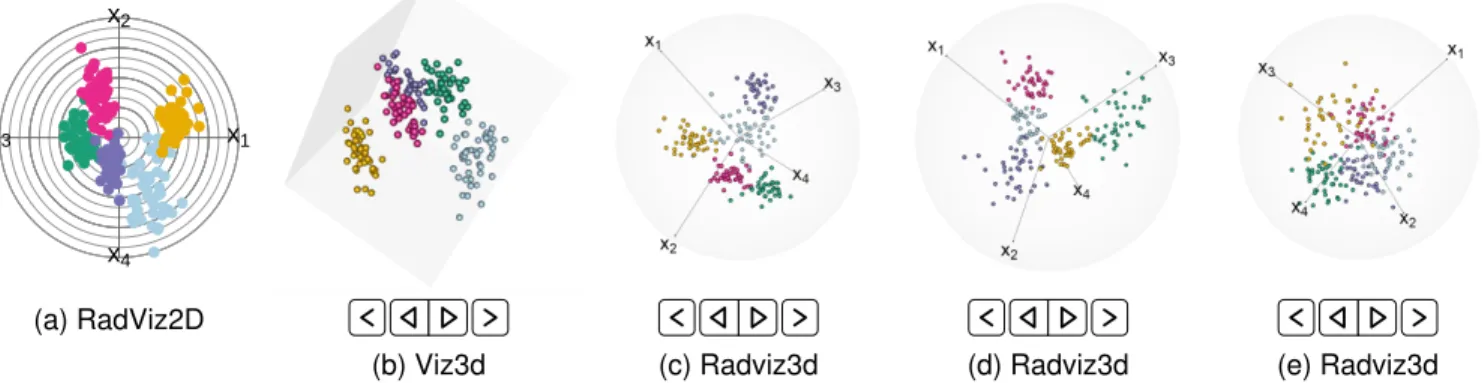
values indicating increased clustering complexity. Figure 1 illustrates visualizations obtained for 4D examples: note that
p= 4is a dimension that allows exact uniform separation of anchor points (Table 1). For these examples, the indi-vidual groups have homogeneous uncorrelated (spherical) dispersions. The first set of figures (Figs. 1a-1c) are for
¨
ω = 0.001 that indexes good separation between groups. However, RadViz2D (Fig. 1a) is not particularly adept at separating out all the classes while Viz3D (Fig. 1b) provides a better representation of the distinctiveness of the groups. However, a more meaningful display is provided by Rad-viz3D (Fig. 1c).We illustrate further the benefits of RadViz3D over Viz3D and RadViz2D by also evaluating their display of simulated datasets with increasing ω¨ (decreasing class separation). Figs. S1d, S1e and 1d display datasets using RadViz2D, Viz3D and RadViz3D for datasets simulated for
¨
ω = 0.01while Figs. S1g, S1h and 1e provide correspond-ing displays for datasets simulated uscorrespond-ing ω¨ = 0.05. The RadViz3D representations of Figs. 1c, 1d and 1e indicate greater difficulty of separation of the groups as we go from
¨
ω = 0.001to 0.01 on to 0.05. Such decreasing separation is more ambiguous with RadViz2D and even so with Viz3D – indeed, the display (Figure S1e) for the dataset simulated for ω¨ = 0.01 does not appear to be qualitatively more separated than that for the dataset withω¨ = 0.05(Fig. 1e). Fig. 1 thus illustrates the benefits of RadViz3D in more accurately displaying grouped multi-dimensional data. Our illustration here is forp = 4that affords the possibility of exactly equi-spaced anchor points, so in Fig. S2, we demon-strate performance by illustrating the three visualization methods on simulated grouped datasets with three different clustering complexities in 5D where Result 1 specifies only approximately equi-spaced anchor points.
2.3 Visualization of High-dimensional Data
With the machinery for 3D radial visualization in place, we turn our attention to summarizing high-dimensional data from multiple groups. It is important to note that for even moderately high dimensions, displaying many anchor points is not possible even after factoring in the benefits of going from 2D to 3D. Additionally our placement of equi-spaced anchor points is built on not inducing spurious positive correlations in the display, and therefore based on the display of coordinates that are far from inducing positive correlations in the display. So we project our high-dimensional datasets into a lower-high-dimensional space such that the projected coordinates are almost uncorrelated. At the same time our objective is to preserve the distinctiveness of groups while finding projections as well as preserving, in the display, the inherent variability in the dataset. A common approach to finding uncorrelated projections is Principal Components Analysis (PCA) that finds the mutu-ally orthogonal projections summarizing a proportion of the total variance in the data. PCA however does not account for class structure in the data and can provide unsatisfactory results for visualization of grouped data when such is ignored, so robust alternatives [46] have been proposed. Our suggestion is to develop the Max-Ratio Projections (MRPs) of the data in order to maximize the separation between groups (in projected space) relative to its total variability. We discuss obtaining these projections next.
x1 x2 x3 x4 ● ● ●●●● ● ● ● ● ● ● ● ● ● ●●●● ● ● ● ● ● ● ● ● ● ● ● ● ● ● ●●●● ● ● ● ● ● ●● ● ● ● ● ● ● ● ● ● ● ● ● ● ● ● ●● ● ● ● ● ● ● ●● ● ● ● ● ● ● ● ● ● ● ● ● ● ● ● ● ● ●● ● ● ● ●●●●● ● ● ● ● ● ●●●●●●●● ● ●●● ● ● ● ● ● ● ● ● ● ● ● ●●● ●●●● ● ● ● ●● ● ●● ● ● ● ● ●● ● ● ● ● ●● ● ● ● ● ● ● ● ● ●●●● ● ● ●● ● ●●● ● ●● ●● ●● ● ●●●●●●● ● ● ●● ● ● ● ● ● ● ● ● ● ● (a) RadViz2D
(b) Viz3d (c) Radviz3d (d) Radviz3d (e) Radviz3d
Fig. 1: Visualizations of 4D datasets using simulated with competing methods using (a-c)ω¨ = 0.001, (d)ω¨ = 0.01and (f)
¨
ω= 0.05. (See also Fig. S1 for a fuller representation that permits a more detailed evaluation.) All 3D displays in this paper are animated for added visualization benefit and viewable with the Adobe Acrobat ReaderTM.
2.3.1 Directions that Maximize Between-Group Variance
Given the group information in our dataset, our objective is to find a linear subspace such that the groups are well-separated when the data are projected along this subspace. Suppose thatv1,v2, . . . ,vkarekuncorrelated direction vec-tors spanning the linear subspace. In order to separate the groups, we want to project the data to eachvjsuch that the
ratio of the projected between-group sum of squares and the total corrected sum of squares is maximized (equivalently, the ratio of the projected within-group sums of squares and the total corrected sum of squares is minimized).
Let Ξ = {X1,X2, . . . ,Xn} be n p-dimensional obser-vation vectors. Then the corrected total sum of squares and cross-products (SSCP) matrix is given by T = (n−1) ˆΣ
where Σˆ is the sample dispersion matrix ofΞ. Now, if Σ
is the dispersion matrix of anyXi, then for any projection vector vj, we have Var(vj0Xi) = vj0Σvj. Further, for any
two vj and vl, Cor(vj0Xi,v0lXi) ∝ vj0Σvl = 0since the
direction vectors decorrelate the observed coordinates. (We may replaceΣwithΣˆ in the expressions above.) Therefore, we obtainv1,v2, . . . ,vk in sequence to satisfy
max v1 SSgroup(v1) SStotal(v1) max vj SSgroup(vj) SStotal(vj) 3 v 0 jT vi= 0, 1≤i < j≤k (5)
whereSStotal(vl)is the corrected total sum of squares of the data projected to the direction vl (so is a scalar quantity),
and SSgroup(vl) is the corrected between-group sum of squares of the data projected to the directionvl.
Result 3. Max-Ratio Projections. LetX1,X2, . . . ,Xn be p-dimensional observations from G groups. Let T be the total corrected SSCP and B be the corrected SSCP between groups. LetT andBboth be positive definite. Then
ˆ vj= T −1 2wˆj kT−12wjˆ k , j= 1,2, . . . , k (6)
satisfies(5)wherewjˆ , j = 1,2, . . . , kare, in decreasing order, theklargest eigenvalues ofT−1/2BT−1/2.
Proof. Let Γg, g = 1,2, . . . , G be the ng ×n matrix that
selects observations from the matrix X that has Xi as its
ith row. Herengis the number of observations from thegth
group, for g = 1,2, . . . , G. Then ΓgX is the matrix with observations from thegth group in its rows and
B=X0 G X g=1 1 ng Γ0g1ng1 0 ngΓg− 1 n1n1 0 n X (7)
andT =X0(In−1n10n/n)X. Also,Xprojected along any
direction v yields SSgroup(v) = v0Bv and SStotal(v) = v0T vso that finding (5) is equivalent to
max v1 v01Bv1 v0 1T v1 max vj v0jBvj v0jT vj v 0 jT vi= 0,1≤i < j≤k. (8)
Letwj=T1/2vj, j = 1,2, . . . , k. Then for eachj, SSgroup(vj) SStotal(vj) = vj0Bvj vj0T vj = w0jT−12BT− 1 2wj w0jwj
andvj0T vi =wj0wi. Then, instead of (8), we can solve the following sequential problems with respect tow1, . . . ,wk:
max w1 w01T− 1 2BT− 1 2w1 w10w1 max wj w0 jT− 1 2BT− 1 2wj w0 jwj 3 w0jwi= 0,1≤i < j≤k. (9)
T−1/2BT−1/2 is nonnegative definite, with at mostG−1
positive eigenvalues, sok≤G−1in (9). The eigenvectors
ˆ
w1,wˆ2, . . . ,wˆkcorresponding to itsklargest eigenvalues in
decreasing order solve (9). Letvjˆ be the normalized version ofT−1/2wˆ
j. Thenvˆjs satisfy (8) and the result follows.
Result 3 provides the projections that maximize the separation between the groups in a lower-dimensional space in a way that also decorrelates the coordinates. The number of projections is limited byG−1. So, forG≤3, 1 to 2 pro-jections and therefore 1D or 2D displays should be enough. (ForG= 3, a RadViz2D figure should normally suffice, but, as we show later in our examples, choosing 4 projections yields a better display even though the additional4−G+ 1
groups. We use springs to provide a physical interpretation for why these additional4−G+1coordinates are beneficial. The firstG−1MRP coordinates pull the data with different forces along the corresponding anchor points in a way that permits maximum separation of the classes. The remaining
4−G+ 1anchor points correspond to the zero eigenvalues and do not contribute to the separation between groups, and so each group is pulled with equal force in the direction of these anchor points. These additional pulls separate the groups better in RadViz3D than in RadViz2D. (We choose 4 MRPs whenG≤4for RadViz3D because a 3D sphere is best separated using 4 equi-spaced anchor points because every axis is then equidistant to the other. For similar reasons, we choose 3 MRPs for 3 anchor points in RadViz2D when
G≤3.) We illustrate this point further in Section 3.2.1. The eigenvalue decomposition of T−1/2BT−1/2
as-sumes a positive definiteT, for which a sufficient condition is thatng> pfor allg. For many high-dimensional datasets,
this assumption may not hold so we now propose to re-duce the dimensionality of the dataset for the cases where
p ≥ mingng while also preserving as far as possible its
group-specific features and variability.
2.3.2 Nearest Projection Matrix to Group-Specific PCs
Our approach builds on standard PCA whose goal, it may be recalled, is to project a dataset onto a lower-dimensional subspace in a way that captures most of its total variance. We use projections that summarize the variability within each group. So, we summarize each group by obtaining PCs separately for the observations in them and then find the closest projection matrix to all the group-specific PCs. Specifically, we have the following
Result 4. Suppose that V1,V2, . . . ,Vm are p× q matrices with Vj0Vj = Iq, where Iq is the q × q identity matrix. Let V = Pmj=1Vj with singular value decomposition (SVD) V =P•Λ•Q0whereP•is ap×qmatrix of orthogonal columns, Qis aq×qorthogonal matrix andΛ•is aq×qdiagonal matrix with v non-zero entries where v = rank(V). Then thep×q matrixW =P•Q0satisfies W = argmin{ m X j=1 kW −Vjk2F :W0W =Iq}. (10)
Proof. MinimizingPmj=1kW −Vjk2F is equivalent to
maxi-mizing Pmj=1trace (W0Vj) or, equivalently, trace (W0V).
Let the full SVD of V = [P•,P◦][Λ•,0]0Q0, where the ith diagonal element of Λ• is the nonnegative eigenvalue
λi. Thentrace (W0V) = trace (Q0W0[P•,P◦][Λ•,0]0). Let B = Q0W0[P•,P◦] have bij as its (i, j)th entry. Then BB0 = Iq and |bij| ≤ 1 for all i, j. So, trace (W0V) ≤
|trace (W0V)| = |Pvi=1λibii| ≤ Pλi|bii| ≤ Pλi = trace (Λ•), with equality holding whenW =P•Q0.
Result 4 reduces the dataset for cases where the number of features is larger than the minimum number of records in any group. We take m = min{p, n1, n2, . . . , ng}. The k
MRPs of our dataset are displayed using RadViz3D. The choice ofkmay be based on the clarity of the display, or by the cumulative proportion (we use 90% in this paper) of the eigenvalues ofT−1/2BT−1/2.
We summarize the steps for obtaining the MRPs of a datasetXas follows:
Algorithm 1Max-Ratio Projection (MRP) Method 1: Remove the group mean for each observation inX. 2: Obtain thep×qeigenvector matricesV1,V2, . . . ,VGfor
each of theGgroups whereq= min{p, n1, n2,· · ·, nG}.
3: Use Result 4 to obtain the nearest orthogonal matrixW
toV1,V2, . . . ,VG.
4: Project the dataset to the new space ofW.
5: Use Result 3 to find the projection matrixV maximizing the between-group variance of the projected data. 6: The matrixXV provides the MRPs of the dataset.
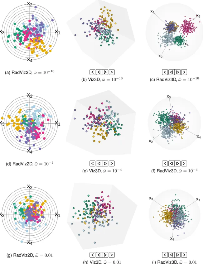
2.3.3 Illustration
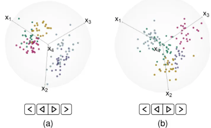
We illustrate performance of Radviz3D on the MRP of 3 MIXSIM-simulated (n = 1000) 500D observations each ob-tained withω¨ ∈ {10−10,10−4,0.01}. For brevity, Fig. 2 only
(a)ω¨ = 0.001 (b)ω¨ = 0.05
Fig. 2: RadViz3D displays of 500D datasets with clustering complexity indexed by (a)ω¨ = 10−10and (b)ω¨ = 0.01.
provides RadViz3D displays of datasets with the least and highest complexity – see Fig. S3 for RadViz2D, Viz3D and Radviz3D visualizations of all three datasets. We see Rad-Viz3D capturing the decreasing separation between groups of observations with increasing ω¨ and doing so better than RadViz2D and Viz3D. Therefore, MRP and RadViz3D together provide an effective display of high-dimensional datasets and convey more accurately relative differences in separation between groups than doing MRP of the dataset when displayed with RadViz2D or Viz3D (Fig. S3). These examples provide some indication of the good performance of RadViz3D in displaying high-dimensional classification datasets with different separation characteristics. We now develop methodology for discrete (and mixed) datasets.
2.4 Visualizing Discrete- and Mixed-Features Datasets
Discrete multivariate datasets are complicated to visualize, but invaluable in applications such as genomics, survey and voting preferences and so on. We visualize them here by transforming them using copulas, specifically constructed to describe the correlation structure among the discrete variables in the joint distribution while maintaining the em-pirical marginal distribution. After transforming discrete-featured datasets to the continuous space, we can apply Section 2.3 for their visualization. We transform the
discrete-features in a dataset via copulas, for which we now intro-duce the generalized distributional transformation.
Definition 5 (Generalized Distributional Transform, [47], Chapter 1). LetY be a real-valued random variable (RV) with cumulative distribution function (CDF)F(·)and letV be a RV independent ofY, such thatV ∼Uniform(0,1). The generalzed distributional transform ofY isU =F(Y, V)whereF(y, λ)=. P(Y < y) +λP(Y =y) =F(y−) +λ[F(y)−F(y−)]is the generalized CDF ofY.
Theorem 6 ([47], Chapter 1). Let U = F(Y, V) be the distributional transform ofY as per Definition 5. Then
U ∼Uniform(0,1) andY =F−1(U) a.s.
where F−1(t) = inf{y ∈ R : F(y) ≥ t} is the generalized inverse, or the quantile transform, ofF(·).
Suppose that Y1,Y2, . . . ,Yn is a sample of discrete-valued random vectors, each of which has the same distribu-tion asξ= (ξ1, ξ2, . . . , ξp), where each marginξihas a CDF Fi(and thus is a step function). LetUi=F(ξi, Vi). Then by
Theorem 6,Ui ∼Uniform(0,1), thus(U1, U2, . . . , Up)∼C
is a copula. Also, the joint distribution forξcan be decom-posed as the marginalsFi’s and the constructed copulaCby
the definition of quantile transform and Theorem 6 again:
F(y1, y2, . . . , yp) =P(ξ1≤y1, ξ2≤y2, . . . , ξp≤yp) =P[Fi−1(Ui)≤yi∀i= 1,2, . . . , p] =P[Ui≤Fi(yi)∀i= 1,2, . . . , p] =C[F1(y1), F2(y2), . . . , Fp(yp)].
Now we may pick p continuous marginal distri-butions, each with CDF F˜i, i = 1,2, . . . , p. Then ( ˜F1−1(U1),F˜2−1(U2), . . . ,F˜p−1(Up)) has a continuous joint
distribution with marginalsF˜i, i= 1,2, . . . , p.
We use the marginal empirical CDF (ECDF)Fˆi(·)of the
Yjs to estimateFi(·)fori = 1,2, . . . , p. We useN(0,1) as
the continuous marginals, i.e.F˜i(·) = Φ(·), theN(0,1)CDF.
We define the Gaussianized-distributional transform (GDT)
G(Yj,Vj) == [[Φ−1( ˆFi(Yji, Vji))]]i=1,2,...,p (11)
for j = 1,2, . . . , n. Here Vj = (Vj1, Vj2, . . . , Vjp), and Vjis are independent identically distributed standard
uni-form realizations. Then Xi = G(Yi,Vi), i = 1,2, . . . , n
are realizations from a multivariate distribution inRp: we
apply the methods of Section 2.3 onX1,X2, . . . ,Xn before visualizing the resulting MRPs using Radviz3D.
Remark 7. We make a few comments on our use of the GDT:
1) For a continuous random variable, Theorem 6 reduces to the usual CDF soG(·,·)can be applied also to datasets with mixed (continuous and discrete) features.
2) The GDT is a more stringent standardization than the usual affine transformation that only sets a dataset to have zero mean and unit variance, because it transforms the marginal ECDFs to Φ(·). So the GDT may, as in Section 3.1.1, also be applied to skewed datasets.
3) When datasets have features with little class-discriminating information, applying the GDT on a dis-crete coordinate will inflate the variance in the trans-formed space, resulting in a standard normal coordinate
that is independent of the other features. When the number of redundant coordinates is substantial relative to group-discriminating features, these independent N(0,1)-transformed coordinates will drive the MRP, resulting in poor separation. We use an analysis of variance (ANOVA) test on each copula-transformed coordinate to ascertain if it contains significant group-discriminating information. We address potential issues of multiple sig-nificance by correcting for false discoveries [48]. Features that fail to reject the null hypothesis are dropped from the MRP steps and the subsequent visualization.
We now summarize the algorithm that combines the GDT and MRP for datasets with discrete or mixed features: Algorithm 2RadViz3D for datasets with discrete, mixed or skewed features
1: Calculate the marginal ECDFFˆ1,Fˆ2, . . . ,Fˆp for each of
thepcoordinates of the dataset. 2: SimulateVi
iid
∼Uniform[0,1]p
.
3: Construct the transform G with marginal ECDFs and simulatedVi, i= 1,2, . . . , n, as in 11.
4: Transform Yi in the discrete dataset to X
¯i with Xi =
G(Yi,Vi), i= 1,2, . . . , n.
5: Apply MRP onXi, i= 1,2, . . . , nviaAlgorithm 1. 6: Display MRP results by RadViz3D.
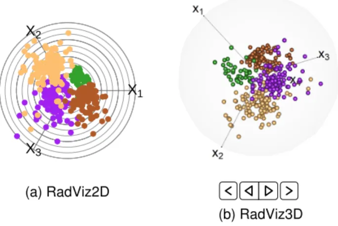
2.4.1 Illustration
We illustrate RadViz3D on the MRPs obtained after GDT on
(a) (b)
Fig. 3: RadViz3D displays of 500D discrete datasets simu-lated with (a) low and (b) high clustering complexity. three 500D datasets of n = 125 observations with binary attributes in each coordinate. We are unaware of a simulator for multivariate discrete datasets that can simulate datasets according to a specific clustering complexity so we use a model developed by K. Dorman where each observation vector is a realization from a first order Markov chain and complexity of the model is governed by the expected num-ber of coordinates that are distinct from each other. Figs. 3 and S4 illustrate performance and shows that RadViz3D displays best the decreasing separation with increasing clus-tering complexity, when compared to Viz3D and Radviz2D, in that order. Our illustrations show that even for discrete datasets, RadViz3D can, after application of the GDT and the MRP, provide a more accurate visualization.
3
R
EAL-D
ATAE
XAMPLESWe illustrate our methodology on datasets with continuous, discrete or mixed features. The focus of our work is on displaying high-dimensional datasets, so we provide only one moderate (9D) example. Our other examples have p
ranging from a few hundred to several thousands. For brevity, we mostly display datasets here with RadViz3D, and refer to the supplement for competing displays.
3.1 Datasets with Continuous Features 3.1.1 A moderate-dimensional dataset
Gamma Ray Bursts (GRBs) are the brighest electromagnetic events known to occur in space and are believed to contain clues to the origin of the cosmos. Although the astrophysics community has long been divided on whether there are two [49] or three [50, 51] kinds of GRBs, a careful recent revisit [52, 53, 54] of the clustering problem revealed that all nine available features are necessary for clustering and show overwhelming evidence of five classes of GRBs. These nine features are the two duration variables that represent the time by which 50% and 90% of the flux arrive, four time-integrated fluences in the 20-50, 50-100,100-300 and
>300 keV spectral channels and three peak fluxes in time bins of 64, 256 and 1024 milliseconds. There are very strong correlations between some of these features, leading to their summary and erroneous [53] deletion before clustering.
Groups 1 2 3 4 5 Fig. 4: RadViz3D display of GRB data
The BATSE 4Br cata-log has complete records on 1599 GRBs. With 9 features, it can concep-tually be displayed us-ing RadViz3D or Viz3D, however we use MRP to project the data onto a lower-dimensional space because of the very strong correlations between the features. The nine features are heavily skewed so we also employ the GDT as per .1) and .2) of Re-mark 7. Fig. 4 displays the dataset using the multi-variate t-mixtures
group-ing [53]. The five groups are not separated with Radviz2D (Fig. S5a) but (as per our 3D animated displays) more separated using Viz3D (Fig. S5b) and even better with RadViz3D. Our display confirms the finding of five distinct classes [53]. At the same time, it also explains the earlier controversy, because it shows two or three possible super-types potentially encompassing the five kinds [53] of GRBs.
3.1.2 High-dimensional Continuous Datasets
We also have illustrations on some very high-dimensional datasets, some of which also haven << pobservations.
3.1.2.1 Zipcode digits
This dataset [55] is of 200016×16images of hand-written Hindu-Arabic numerals (from 0 to 9) and has been used to evaluate classification and clustering algorithms. Fig. 5a displays a sample of 20% of these numerals. The marginal
(a) Random sample of
zip-code digits dataset (b) Radviz3d Digits 0 1 2 3 4 5 6 7 8 9
Fig. 5: (a) Sample and (b) RadViz3D display of zipcode data. distribution at each pixel is unclear, so we use the GDT before obtaining the MRPs. Figs. S6a, S6b and 5b provide RadViz2D, Viz3D and RadViz3D displays of the 4 MRPs of the zip code dataset. The largeG, widely varying frequency of occurrence of each digit, and more importantly, hand-writing variability makes separating all the digits difficult. Nevertheless, RadViz3D distinguishes 0s and 6s from the others very well. Also, 1s are separated from most other digits, while 3s are also well-separated but overlap the 5s and 8s. Therefore, while not all digits are easily separated in any of the three displays, RadViz3D is the best performer.
3.1.2.2 Faces
TheFacesdataset [56] has112×92images of 40 human faces taken at 10 different light angles and conditions. We choose the 10 faces of 6 people (Fig.6a) for our illustration. We apply the wavelet transform on the Radon projection of each image [57] to address variations in facial expression, and illumination and use these reduced 280 features for our displays. The Radon projections and wavelet transfors yield
(a)
(b) Person A B C D E F
Fig. 6: (a) The set of faces and (b) its RadViz3D display. unclear marginal distributions so we use the GDT before obtaining the MRPs. The RadViz2D (Fig. S7a) only identifies Persons A and B from the others while Viz3D (Fig. S7b)
also clarifies Persons C and F. Radviz3D (Fig. 6b) is the best performer in distinguishing the six subjects.
3.1.2.3 Suicide ideation
Predicting suicide is a challenging task for psychia-trists. A recent functional Magnetic Resonance Imaging study [58] identified 6 (out of 30) words that distinguished
Non-suicidal controls Suicidal attempters Suicidal non-attempters Fig. 7: Suicide ideation dataset. 9 suicide attempters and
8 non-attempter ideators based on changes in ac-tivation. The study also included scans on 17 healthy controls with no personal or family his-tory of psychiatric disor-ders or suicide attempts. Our dataset therefore has
G=3groups of responses (changes in activation, rel-ative to the baseline) to these six words (which we consider as replicates) at p = 70150 voxels. Fig. 7 shows that Rad-Viz3D considerably sep-arates the control group from the suicide ideators,
and even reasonably distinguishes the attempters from the attempters. The ambiguity between ideator non-attempters and non-attempters is an indicator of the challenges in predicting suicide, but the RadViz3D display is clearer than with RadViz2D (Fig. S8a) or Viz3D (Fig. S8b).
For this dataset G= 3 so only 2 MRPs are possible, allowing us to independently assess MRP and RadViz3D. Fig. S8d shows the 3 groups as fairly well-separated by lin-ear decision rules. RadViz3D needs 2 more projections with zero eigenvalues for optimal display while RadViz2D and Viz3D need only an additional such projection. However, Figs. S8a and S8b show less clarity than RadViz3D (Fig. 7).
3.2 Datasets with Discrete Features
Our next examples are on datasets with discrete features.
3.2.1 Voting Records of US Senators
Democratic Republican Fig. 8: RadViz3D display of senators’ voting records. The 108th US Congress
had 55 Republican and 45 Democratic (including 1 independent in the Democratic caucus) senators vote on 542 bills [59]. We display the senators according to whether they voted for each bill or not (i.e.
against/abstained). The RadViz3D (Fig. 8) display distinguishes the 2 groups of senators better than RadViz2D (Fig. S9a) or Viz3D (Fig. S9b). Here
G=2, so 3 zero-eigenvalue
projections beyond the MRP are used in the RadViz3D display. These additional projections (associated with the anchor points X2, X3, X4) do not contribute towards separating the 2 groups which are separated solely by the first MRP (associated withX1). A physical interpretation is that the spring on anchor pointX1 pulls one group harder than another group, separating it out, while the “null” springs onX2, X3, X4pull both groups with equal force. A
similar interpretation applies to the forces of the two null springs (X2, X3) of the RadViz2D and Viz3D displays but RadViz3D performs better, perhaps because each spring has a larger domain of influence in the 3D volume.
3.2.2 Autism Spectrum Disorder (ASD) Screening
Normal ASD subject Fig. 9: RadViz3D display of the ASD screening dataset. This dataset [60] from the
UCI’s Machine Learning Repository (MLR) [61] has 15 binary (and 5 addi-tional) features on 515 normal and 189 ASD-diagnosed adults. Fig. 9 is a RadViz3D display of the binary attributes. Corresponding RadViz2D and Viz3D displays are in Figs. S10a and S10b. Rad-Viz3D best distinguishes the 2 groups and points to the possibility of us-ing the screening fea-tures to assess difficult-to-diagnose [60] ASD.
3.2.3 SPECT Heart
Dataset
This dataset [62] from the UCIMLR [61] has 22 binary
Normal Abnormal Fig. 10: RadViz3D display of the SPECT Heart dataset. attributes that summarize
cardiac Single Proton Emission Computed Tomography (SPECT) images of 55 normal and 212 abnormal patients. Figs. 10, S11a and S11b provide RadViz3D, RadViz2D and Viz3D displays of the patients. The use of GDT and MRP have resulted in a dataset with easily-separated groups, but here also RadViz3D is the best performer, followed by Viz3D and RadViz2D.
Our illustrative exam-ples show that RadViz3D,
along with the GDT and the MRP can be used to effectively display grouped data with discrete numerical features.
3.3 Datasets with mixed features
The development of Section 2.4 is general enough to ex-tend to datasets with continuous and numerical
discrete-valued features. We now illustrate performance on two such datasets.
3.3.1 Indic scripts
This dataset [63] is on 116 different features from hand-written scripts of 11 Indic languages. We choose a subset of 5 languages from 4 regions, namely Bangla (from the east), Gurmukhi (north), Gujarati (west), and Kannada and Malayalam (languages from the neighboring southern states of Karnataka and Kerala) and a sixth language (Urdu, with a distinct Persian script). Figure. 11a displays a line from a sample document in each script and illustrates the chal-lenges in characterizing handwritten scripts because of the additional effect of individual handwriting styles. Figs. 11b
(a) Handwriting samples from (top to bottom) Bangla, Gujarati, Gurmukhi, Kannada, Malayalam and Urdu
(b) Viz3D (c) RadViz3D
Bangla Gujarati Gurmukhi Kannada Malayalam Urdu
Fig. 11: Viz3D and RadViz3D display of Indic scripts dataset. and 11c provide Viz3D and RadViz3D displays of the reduced dataset (see Fig. S12a for the RadViz2D display). Viz3D (and to a lesser extent RadViz2D) separates Urdu, Kannada and Gujarati very well but does not distinguish the other 3 languages. On the other hand, RadViz3D is the best performer in terms of clarifying the 6 scripts.
We also separately displayed documents in the 4 south Indian scripts of Kannada, Malayalam, Tamil and Telugu. With G = 4, only 3 MRPs are possible, so this example is a case where RadViz2D and Viz3D may perform bet-ter given that there is no need for any additional zero-eigenvalue projections, while RadViz3D needs one such
X1 X2 X3 ● ● ●● ● ●● ● ● ●●●●●●● ● ●● ● ●● ● ● ● ● ● ● ● ●●●● ● ● ●● ● ●●●● ●● ●● ● ● ● ●● ●● ●● ● ●● ● ● ● ●● ● ● ● ●● ● ● ●● ● ● ● ● ● ● ● ●●● ● ● ● ● ● ● ● ●●● ●●●●● ● ● ● ● ● ● ● ● ● ● ● ●● ●● ● ● ● ● ● ● ● ●●●● ● ● ● ● ● ● ● ● ● ●●●●●●●●●●●● ●● ● ● ●●●●● ● ● ● ● ● ● ● ● ●● ● ● ● ● ● ● ● ● ● ● ● ● ●● ● ● ● ● ● ● ● ● ● ● ● ● ● ● ● ● ● ● ● ● ● ● ● ● ● ● ● ● ● ● ● ● ● ● ●●● ●●● ● ● ● ● ●● ● ● ●●● ●●● ● ● ● ● ● ●● ● ●●●● ● ● ● ●● ● ● ●●● ● ● ● ● ● ● ●● ● ● ●● ●●●● ● ● ● ● ● ● ● ●● ● ● ● ● ● ● ●●●●●● ● ● ● ● ● ● ● ●● ● ●● ● ●●● ● ● ● ● ● ● ● ●● ●● ● ● ● ● ●●●● ● ● ● ● ● ● ● ● ● ●● ● ● ● ● ● ● ●●● ● ●● ● ● ●● ●● ● ●● ● (a) RadViz2D (b) RadViz3D Kannada Malayalam Tamil Telugu
Fig. 12: (a) RadViz2D and (b) RadViz3D displays of the 4 southern Indic-scripts dataset.
projection for display. However, Figs. 12 and S13 show that RadViz2D (Fig. S13a) and Viz3D (Fig. S13b) displays do a poorer job in separating out the 4 languages than RadViz3D (Fig. 12b). We surmise that this is because of the additional volume made available by the fully 3D rendering provided by RadViz3D relative to RadViz2D and Viz3D.
3.3.2 RNA sequences of human tissues
This dataset [64] consists of gene expression levels, in FPKM
Breast Colon Esophagus Liver Lung Prostate Stomach Thyrioid
Fig. 13: The RNA-seq dataset. (Fragments per Kilobase
of transcripts per Mil-lion), of RNA sequences from 13 human organs of which we choose the eight largest (in terms of available samples) for our illustration. These are the esophagus (659 sam-ples), colon (339), thyroid (318), lung (313), breast (212), stomach (159), liver (115) and prostate (106). For this dataset, there are
p=20242discrete features, however some of them have so many discrete val-ues so as to essentially be continuous, which means a dataset of mixed
at-tributes. Fig. 13 provides the RadViz3D display that in-dicates very clear separation between the organs, ex-cept for the prostate and the stomach which have some marginal overlap. In contrast, RadViz2D (Fig. S14a) and Viz3D (Fig. S14b) are far poorer at separating out tissue samples from the different organs.
Our detailed evaluations here show the ability of Rad-Viz3D to display high-dimensional grouped data, when used in conjunction with the GDT and the MRP.
4
C
ONCLUSIONS ANDF
UTURE APPLICATIONSWe develop a 3D radial visualization tool called RadViz3D that provides a more comprehensive display of grouped data than does classic 2D RadViz (called RadViz2D here) and its current 3D extension (Viz3D). Our particular interest in this paper is in the display of high-dimensional grouped datasets, for which we develop the MRP to summarize a dataset before display. Further, datasets with numeri-cal discrete-valued, mixed or heavily-skewed attributes are transformed to the continuous space using the GDT, follow-ing which they are displayed usfollow-ing the MRP and RadViz3D, after removing redundant features. Our methodology per-forms well in displaying distinct groups of observations. A R[43] package https://github.com/fanne-stat/radviz3d/ implementing our methodology is also provided.
A number of aspects of our development could benefit from further attention. For instance, the MRP is a linear projection method that is designed to maximize separation between grouped data. It would be interesting to see if non-linear projections can provide improved results. Also our displays have been developed in the context of maximizing distinctiveness of classes. Our methodology is also general to apply for the display of data where there is no class information. In that case, other summaries than the MRP can be used. Also, the GDT is inapplicable to datasets with fea-tures that have more than two nominal categories. It would be important to develop methodology for such datasets. Further, the GDT and the MRP are general transformation and data reduction methods that can be used with other vi-sualization techniques. It would also be worth investigating whether other visualization tools using these methods can better display datasets in some cases. Our development of RadViz3D uses (at least approximately) equi-spaced anchor points. It would be interesting to see if layouts and spacings such as done [32, 34, 35] for RadViz2D can be developed for improved displays and interpretations. Thus, we see that while we have made an important contribution towards the 3D radial visualization tool for high-dimensional datasets, many issues meriting additional investigation and develop-ment remain.
A
CKNOWLEDGMENTSThe authors thank Somak Dutta, Niraj Kunwar, Huong Nguyen, Pu Lu, Fernando Silva Aguilar, Gani Agadilov and Isaac Agbemafle for helpful discussions on earlier versions of this manuscript. R. Maitra’s research was supported in part by the National Institute of Biomedical Imaging and Bioengineering (NIBIB) of the National Institutes of Health (NIH) under its Award No. R21EB016212, and by the United States Department of Agriculture (USDA)/National Institute of Food and Agriculture (NIFA), Hatch project IOW03617. The content of this paper however is solely the responsibility of the authors and does not represent the official views of either the NIBIB, the NIH or the USDA.
R
EFERENCES[1] R. Mead, R. N. Curnow, and A. M. Hasted,Statistical Methods in Agriculture and Experimental Biology, 3rd ed. New York: Chapman and Hall/CRC, 2003.
[2] C. J. Kowalski, “A commentary on the use of multi-variate statistical methods in anthropometric research,”
American Journal of Physical Anthropology, vol. 36, pp. 119–132, 1972.
[3] A. A. Goodman, “Principles of high-dimensional data visualization in astronomy,” Astronomische Nachrichten, vol. 333, no. 5-6, pp. 505–514, 2012. [Online]. Available: https://onlinelibrary.wiley.com/ doi/abs/10.1002/asna.201211705
[4] P. G. N. Digby and R. A. Kempton,Population and Com-munity Biology Series: Multivariate Analysis of Ecological Communities. London: Chapman and Hall, 1987. [5] K. Yang and J. Trewn,Multivariate Statistical Methods in
Quality Management. New York: McGraw-Hill, 2004. [6] A. Malovini, R. Bellazzi, C. Napolitano, and G.
Guf-fanti, “Multivariate methods for genetic variants se-lection and risk prediction in cardiovascular diseases,”
Frontiers in Cardiovascular Medicine, vol. 3, no. 1, 2016. [7] J. C. Davis,Statistics and Data Analysis in Geology. New
York: Wiley, 1986.
[8] J. Clinton, S. Jackman, and D. Rivers, “The statistical analysis of roll call data,” American Political Science Review, p. 355–370, 2004.
[9] N. H. Timm, Multivariate Analysis with Applica-tions in Education and Psychology. Monterrey, CA: Brooks/Cole, 1975.
[10] P. R. Stopher and A. H. Meyburg,Survey Sampling and Multivariate Analysis for Social Scientists and Engineers. Lexington, MA: Lexington Books, 1979.
[11] R. Maitra, “Clustering massive datasets with applica-tions to software metrics and tomography,” Technomet-rics, vol. 43, no. 3, pp. 336–346, 2001.
[12] R. A. Fisher, “The use of multiple measurements in taxonomic poblems,”Annals of Eugenics, vol. 7, pp. 179– 188, 1936.
[13] F. C. James and C. E. McCulloch, “Multivariate analysis in ecology and systematics: Panacea or pandora’s box?”
Annual Reviews in Ecology and Systematics, vol. 21, pp. 129–166, 1990.
[14] S. K. Card, J. D. Mackinlay, and B. Schneiderman,
Readings in information visualization: using vision to think. Morgan Kaufmann, 1999.
[15] E. Bertini, A. Tatu, and D. Keim, “Quality metrics in high-dimensional data visualization: an overview and systematization,”IEEE Transactions on Visualization and Computer Graphics, vol. 17, no. 12, p. 2203–2212, 2011. [16] J. M. Chambers, W. S. Cleveland, B. Kleiner, and P. A.
Tukey,Graphical Methods for Data Analysis. Belmont, CA: Wadsworth, 1983.
[17] H. Chernoff, “The use of faces to represent points in k-dimensional space graphically,”Journal of the American Statistical Association, vol. 68, no. 342, pp. 361–368, 1973. [18] A. Inselberg, “The plane with parallel coordinates,”The
Visual Computer, vol. 1, pp. 69–91, 1985.
[19] E. Wegman, “Hyperdimensional data analysis using parallel coordinates,”Journal of the American Statistical Association, vol. 85, pp. 664–675, 1990.
[20] U. Fayyad, G. Grinstein, and A. Wierse, Information Visualization in Data Mining and Knowledge Discovery. Morgan Kaufmann, 2001.
[21] D. F. Andrews, “Plots of high-dimensional data,” Bio-metrics, vol. 28, no. 1, pp. 125–136, 1972.
multi-variate data: Some new suggestions and applications,”
Journal of Statistical Planning and Inference, vol. 100, no. 2, pp. 411–425, 2002.
[23] E. Kandogan, “Visualizing multi-dimensional clusters, trends, and outliers using star coordinates,” in
Proceedings of the Seventh ACM SIGKDD International Conference on Knowledge Discovery and Data Mining, ser. KDD ’01. New York, NY, USA: ACM, 2001, pp. 107–116. [Online]. Available: http://doi.acm.org/10. 1145/502512.502530
[24] T. van Long and L. Linsen, “Visualizing high den-sity clusters in multidimensional data using optimized star coordinates,” Computational Statistics, vol. 26, p. 655–678, 2011.
[25] S. C. Tan and J. Tan, “Lost in translation: The fundamental flaws in star coordinate visualizations,”
Procedia Computer Science, vol. 108, pp. 2308 – 2312, 2017, international Conference on Computational Sci-ence, ICCS 2017, 12-14 June 2017, Zurich, Switzerland. [Online]. Available: http://www.sciencedirect.com/ science/article/pii/S1877050917306270
[26] P. Hoffman, G. Grinstein, K. Marx, I. Grosse, and E. Stanley, “DNA visual and analytic data mining,” in Proceedings of the 8th conference on Visualization ’97, VIS’97. IEEE Computer Society Press, 1997, p. 437–441. [27] P. Hoffman, G. Grinstein, and D. Pinkney, “Dimen-sional anchors: a graphic primitive for multidimen-sional multivariate information visualizations,” in Pro-ceedings of the 1999 workshop on new paradigms in infor-mation visualization and manipulation in conjunction with the eighth ACM internation conference on Information and knowledge management. ACM, 1999, pp. 9–16.
[28] G. G. Grinstein, C. B. Jessee, P. E. Hoffman, P. J. O’Neil, and A. G. Gee, “High-dimensional visualization sup-port for data mining gene expression data,” in DNA Arrays: Technologies and Experimental Strategies, E. V. Grigorenko, Ed. Boca Raton, Florida: CRC Press LLC, 2001, ch. 6, pp. 86–131.
[29] G. M. Draper, Y. Livnat, and R. F. Riesenfeld, “A sur-vey of radial methods for information visualization,”
IEEE Transactions on Visualization and Computer Graphics, vol. 15, no. 5, pp. 759–776, Sep. 2009.
[30] M. Rubio-S´anchez, L. Raya, F. Diaz, and A. Sanchez, “A comparative study between radviz and star coor-dinates,”IEEE transactions on visualization and computer graphics, vol. 22, no. 1, pp. 619–628, 2016.
[31] L. Nov´akov´a and O. ˇStepankov´a, “Radviz and identifi-cation of clusters in multidimensional data,” in13th In-ternational Conference on Information Visualisation. IEEE, 2009, pp. 104–109.
[32] L. di Caro, V. Frias-Martinez, and E. Frias-Martinez, “Analyzing the role of dimension arrangement for data visualization in Radviz,” inAdvances in Knowledge Discovery and Data Mining. Springer, 2010, p. 125–132. [33] K. Daniels, G. Grinstein, A. Russell, and M. Glidden, “Properties of normalized radial visualizations,”
Information Visualization, vol. 11, no. 4, pp. 273–300, 2012. [Online]. Available: https://doi.org/10.1177/ 1473871612439357
[34] T. van Long and V. T. Ngan, “An optimal radial lay-out for high dimensional data class visualization,” in
2015 International Conference on Advanced Technologies for Communications (ATC), 2015, pp. 343–346.
[35] S. Cheng, W. Xu, and K. Mueller, “Radviz Deluxe: An attribute-aware display for multivariate data,” Pro-cesses, vol. 5, p. 75, 2017.
[36] A. O. Artero and M. C. F. de Oliveira, “Viz3d: effective exploratory visualization of large multidimensional data sets,” in Proceedings. 17th Brazilian Symposium on Computer Graphics and Image Processing, Oct 2004, pp. 340–347.
[37] M. Ankerst, D. Keim, and H. P. Kriegel, “Circle seg-ments: a technique for visually exploring large multi-dimensional data sets,”Human Factors, vol. 1501, pp. 5–8, 1996.
[38] J. Sharko, G. Grinstein, and K. A. Marx, “Vectorized Radviz and its application to multiple cluster datasets,”
IEEE Transactions on Visualization and Computer Graphics, vol. 14, no. 6, pp. 1444–1451, December 2008.
[39] A. Gonz´alez, “Measurement of areas on a sphere using fibonacci and latitude-longitude lattices,”Mathematical Geosciences, vol. 42, p. 49, january 2010.
[40] M. Atiyah and P. Sutcliffe, “Polyhedra in physics, chemistry and geometry,”Milan Journal of Mathematics, vol. 71, no. 1, pp. 33–58, Sep 2003. [Online]. Available: https://doi.org/10.1007/s00032-003-0014-1
[41] E. B. Saff and A. B. Kuijlaars, “Distributing many points on a sphere,”The mathematical intelligencer, vol. 19, dec 1997.
[42] V. Melnykov, W.-C. Chen, and R. Maitra, “MixSim: An R package for simulating data to study performance of clustering algorithms,”Journal of Statistical Software, vol. 51, no. 12, pp. 1–25, 2012. [Online]. Available: http://www.jstatsoft.org/v51/i12/
[43] R Development Core Team, “R: A language and environment for statistical computing,” R Foundation for Statistical Computing, Vienna, Austria, 2018, ISBN 3-900051-07-0. [Online]. Available: http://www. R-project.org
[44] R. Maitra and V. Melnykov, “Simulating data to study performance of finite mixture modeling and cluster-ing algorithms,”Journal of Computational and Graphical Statistics, vol. 19, no. 2, pp. 354–376, 2010.
[45] V. Melnykov and R. Maitra, “CARP: Software for fish-ing out good clusterfish-ing algorithms,”Journal of Machine Learning Research, vol. 12, pp. 69 – 73, 2011.
[46] Y. Koren and L. Carmel, “Robust linear dimensionality reduction,”IEEE Transactions on Visualization and Com-puter Graphics, vol. 10, no. 4, pp. 459–470, July 2004. [47] L. R ¨uschendorf, Mathematical Risk Analysis. Berlin
Heidelberg: Springer-Verlag, 2013.
[48] Y. Benjamini and Y. Hochberg, “Controlling the false discovery rate: a practical and powerful approach to multiple testing,”Journal of the Royal Statistical Society, vol. 57, pp. 289–300, 1995.
[49] C. Kouveliotou, C. A. Meegan, G. J. Fishman, N. P. Bhat, M. S. Briggs, T. M. Koshut, W. S. Paciesas, and G. N. Pendleton, “Identification of two classes of gamma-ray bursts,”Astrophysical Journal Letters, vol. 413, pp. L101– L104, Aug. 1993.
[50] S. Mukherjee, E. D. Feigelson, G. Jogesh Babu, F. Murtagh, C. Fraley, and A. Raftery, “Three Types of
Gamma-Ray Bursts,”Astrophysical Journal, vol. 508, pp. 314–327, Nov. 1998.
[51] I. Horv´ath, “A further study of the batse gamma-ray burst duration distribution,” Astronomy and Astrophysics, vol. 392, no. 3, pp. 791–793, 2002. [On-line]. Available: http://dx.doi.org/10.1051/0004-6361: 20020808
[52] S. Chattopadhyay and R. Maitra, “Gaussian-mixture-model-based cluster analysis finds five kinds of gamma-ray bursts in the batse catalogue,” Monthly Notices of the Royal Astronomical Society, vol. 469, no. 3, pp. 3374–3389, 2017. [Online]. Available: +http://dx.doi.org/10.1093/mnras/stx1024
[53] ——, “Multivariate t-Mixtures-Model-based Cluster Analysis of BATSE Catalog Establishes Importance of All Observed Parameters, Confirms Five Distinct Ellipsoidal Sub-populations of Gamma Ray Bursts,”
Monthly Notices of the Royal Astronomical Society, vol. 481, no. 3, pp. 3196–3209, Dec. 2018.
[54] I. Almod ´ovar-Rivera and R. Maitra, “Kernel Nonpara-metric Overlap-based syncytial clustering,” ArXiv e-prints, may 2018.
[55] W. Stuetzle and R. Nugent, “A generalized single link-age method for estimating the cluster tree of a density,”
Journal of Computational and Graphical Statistics, 2010. [56] F. S. Samaria and A. C. Harter, “Parameterisation of
a stochastic model for human face identification,” in
Proceedings of 1994 IEEE Workshop on Applications of Computer Vision, Dec 1994, pp. 138–142.
[57] D. V. Jadhav and R. S. Holambe, “Feature extraction using radon and wavelet transforms with application to face recognition,”Neurocomputing, vol. 72, no. 7, pp. 1951 – 1959, 2009, advances in Machine Learning and Computational Intelligence. [Online]. Available: http://www.sciencedirect.com/ science/article/pii/S0925231208003135
[58] M. Adam Just, L. Pan, V. L. Cherkassky, D. L. McMakin, C. Cha, M. Nock, and D. Brent, “Machine learning of neural representations of suicide and emotion concepts identifies suicidal youth,” Nature Human Behaviour, vol. 1, pp. 911–919, 12 2017.
[59] O. Banerjee, L. E. Ghaoui, and A. d’Aspremont, “Model selection through sparse maximum likelihood estima-tion for multivariate gaussian or binary data,”Journal of Machine Learning Research, vol. 9, pp. 485–516, 2008. [60] F. Thabtah, “Autism spectrum disorder screening:
ma-chine learning adaptation and DSM-5 fulfillment,” in
Proceedings of the 1st International Conference on Medical and Health Informatics 2017. ACM, 2017, pp. 1–6. [61] D. J. Newman, S. Hettich, C. L. Blake, and C. J.
Merz, “UCI repository of machine learning databases,” 1998. [Online]. Available: http://www.ics.uci.edu/$\ sim$mlearn/MLRepository.html
[62] L. A. Kurgan, K. J. Cios, R. Tadeusiewicz, M. R. Ogiela, and L. S. Goodenday, “Knowledge discovery approach to automated cardiac SPECT diagnosis,”Artificial Intel-ligence in Medicine, vol. 23, no. 2, pp. 149–169, 2001. [63] S. M. Obaidullah, C. Halder, K. C. Santosh, N. Das,
and K. Roy, “Phdindic 11: page-level handwritten document image dataset of 11 official indic scripts for script identification,”Multimedia Tools and Applications,
vol. 77, no. 2, pp. 1643–1678, Jan 2018. [Online]. Available: https://doi.org/10.1007/s11042-017-4373-y [64] Q. Wang, J. Armenia, C. Zhang, A. Penson, E. Reznik, L. Zhang, T. Minet, A. Ochoa, B. Gross, C. A. Iacobuzio-Donahue, D. Betel, B. S. Taylor, J. Gao, and N. Schultz, “Unifying cancer and normal RNA sequencing data from different sources,”Scientific Data, vol. 5, p. 180061, 04 2018.
x
1x
2x
3x
4 ● ● ●●●● ● ● ● ● ● ● ● ● ● ●●●● ● ● ● ● ● ● ● ● ● ● ● ● ● ● ●●●● ● ● ● ● ● ●● ● ● ● ● ● ● ● ● ● ● ● ● ● ● ● ● ● ● ● ● ● ● ● ●● ● ● ● ● ● ● ● ● ● ● ● ● ● ● ● ● ● ●● ● ● ● ●●● ● ● ● ● ●● ● ●●●●● ● ●● ● ●●● ● ● ● ● ● ● ● ● ● ● ● ●●● ●●●● ● ● ● ● ● ● ●● ● ● ● ● ●● ● ● ● ● ●● ● ● ● ● ● ● ● ● ●● ● ● ● ● ● ● ● ●●● ● ●● ●● ●● ● ●●●●●● ●● ● ●● ● ● ● ● ● ● ● ● ● ● (a) RadViz2D (b) Viz3D (c) RadViz3Dx
1x
2x
3x
4 ● ● ● ● ● ● ● ● ● ● ● ● ● ● ● ● ● ● ●● ● ● ● ● ● ● ●● ● ● ● ● ● ● ● ● ● ● ● ● ● ● ● ● ● ● ● ●●● ●●● ●●●●● ● ●● ●● ● ●● ● ●●● ● ● ● ● ● ● ● ● ● ● ● ● ● ● ● ● ● ●● ● ● ● ● ● ● ● ● ● ● ●● ● ● ● ● ● ●●● ● ● ● ● ● ● ● ● ● ● ● ● ● ● ● ● ● ● ● ● ● ● ●●●● ● ● ● ● ● ● ● ● ● ● ● ● ● ● ● ●●●●● ● ●● ● ● ● ● ● ● ● ● ● ● ● ● ● ● ● ● ● ● ● ● ● ● ● ● ●● ● ● ● ● ● ● ● ● ● ● ● ● ● ● ● ● (d) RadViz2D(e) Viz3D (f) RadViz3D
x
1x
2x
3x
4 ● ● ● ● ●● ● ● ● ●● ● ● ● ● ● ● ●● ● ● ● ● ●●●● ● ● ● ● ● ● ● ● ● ● ● ● ● ● ● ● ● ● ● ● ● ● ●●●● ● ●● ●● ● ● ● ● ● ●● ● ● ● ● ● ● ●● ● ● ● ● ● ● ● ● ● ● ● ● ● ● ●● ● ● ● ●● ● ● ●● ● ● ● ● ● ●●● ● ● ● ● ● ● ● ●● ● ● ● ● ● ● ● ● ● ● ● ● ● ● ● ● ● ● ● ● ● ●● ● ● ● ● ● ● ● ● ●● ● ● ● ● ● ● ● ● ● ● ● ● ● ● ● ● ● ● ● ●● ● ● ● ● ● ● ● ● ● ● ● ● ● ● ● ●● ● ● ● ● ● ● ● ● ● ● ● ● ● ● (g) RadViz2D(h) Viz3D (i) RadViz3D
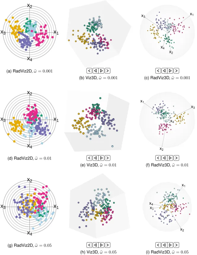
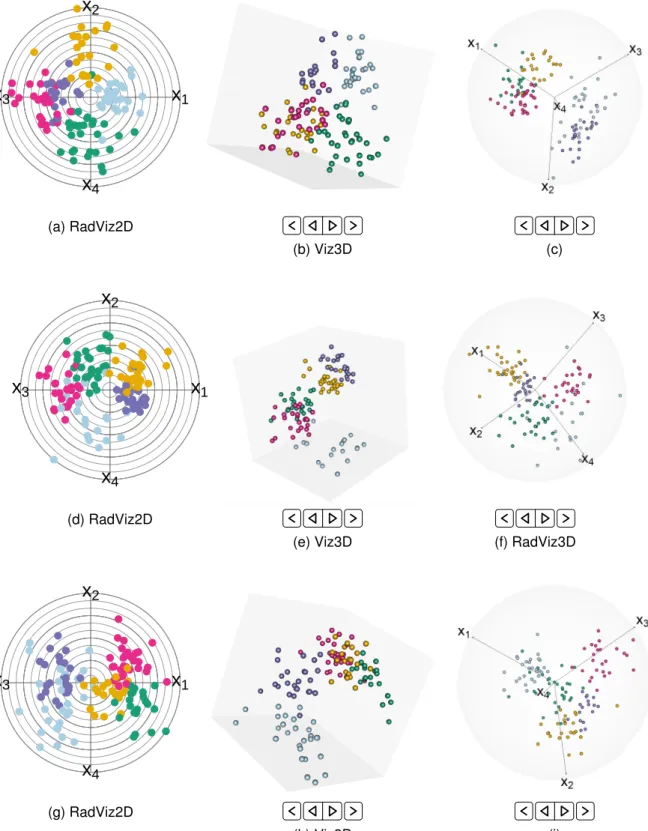
Fig. S1: RadViz2D, Viz3D and RadViz3D of 4D datasets simulated with (a-c)ω¨ = 0.001, (d-f)ω¨ = 0.01and (g-i)ω¨ = 0.05. We display all figures in the supplement to permit easier comparisons.
x
1x
2x
3x
4 ● ● ● ● ● ●● ● ●● ● ● ● ● ● ● ● ● ● ● ● ● ● ● ● ● ● ● ● ●● ● ● ● ●● ● ● ● ● ● ● ● ● ● ● ● ● ● ● ● ● ● ● ● ● ● ●● ● ● ● ● ● ● ● ● ● ● ● ●● ● ● ●● ● ● ● ● ● ● ● ● ● ●● ● ● ●● ● ● ● ● ●● ● ● ● ● ● ● ● ● ● ● ● ● ● ● ●●● ● ● ●● ● ● ● ●● ● ● ● ● ● ●● ● ● ● ● ● ● ● ● ● ● ● ● ● ● ● ● ● ● ● ● ● ● ● ● ●● ● ● ● ● ● ● ● ● ● ● ● ● ● ● ● ● ● ● ● ● ● ● ● ● ● ● ● ● ● ● ● ● ●● ● ● ● ● ● ● ● ● ● ● (a) RadViz2D,ω¨ = 0.001 (b) Viz3D,ω¨ = 0.001 (c) RadViz3D,ω¨ = 0.001x
1x
2x
3x
4 ● ● ● ● ● ● ● ● ● ● ● ● ● ● ● ● ● ●● ● ● ● ● ● ●● ● ● ●● ●● ● ● ● ● ● ● ● ● ● ● ● ● ● ● ● ● ● ● ● ● ● ● ● ● ● ● ● ● ● ● ● ● ● ● ● ● ● ● ● ● ● ● ● ● ● ● ● ● ● ● ● ●● ● ● ● ● ● ● ● ● ● ● ● ● ● ● ● ● ● ● ● ● ● ● ● ● ● ● ● ● ● ● ● ●● ● ● ● ● ● ● ● ● ● ●●●● ● ● ● ● ●● ● ● ● ● ● ● ● ● ● ● ● ● ●●● ●● ● ● ● ● ● ● ● ● ● ● ●● ● ● ● ● ● ● ● ● ● ● ● ● ● ● ● ● ●● ● ● ● ● ● ● ● ● ● ● ● ● ● ● ● ● (d) RadViz2D,ω¨ = 0.01(e) Viz3D,ω¨ = 0.01 (f) RadViz3D,ω¨ = 0.01
x
1x
2x
3x
4 ● ● ● ● ● ● ●● ● ● ● ● ● ● ● ● ● ● ● ● ● ● ● ● ● ● ● ● ● ● ● ● ● ● ● ● ● ● ● ● ● ● ● ● ● ● ● ● ● ●● ● ● ● ● ● ● ● ● ● ● ● ● ● ● ● ● ● ● ● ● ● ● ● ● ●● ● ● ● ● ● ● ● ● ● ● ● ● ● ● ● ● ● ● ● ● ● ● ● ● ● ● ● ● ● ● ● ● ● ● ● ● ● ● ● ● ● ● ● ● ● ● ● ● ● ●● ● ● ● ● ● ● ●● ●● ● ● ● ● ● ● ● ● ● ● ● ● ● ● ● ● ● ● ● ● ●● ● ● ● ● ● ● ● ● ● ● ● ● ● ● ● ● ● ● ● ● ● ● ● ● ● ●● ● ● ● ● ● ● ● ● ● ● ● ● ● (g) RadViz2D,ω¨ = 0.05(h) Viz3D,ω¨ = 0.05 (i) RadViz3D,ω¨ = 0.05
x
1x
2x
3x
4 ● ● ● ● ● ● ● ● ● ● ● ● ● ● ● ● ● ● ● ● ●● ● ● ● ●● ● ● ● ● ●● ● ● ● ● ● ● ● ● ● ● ● ● ● ● ● ● ● ● ● ● ●● ● ● ● ● ● ● ● ●● ● ● ● ● ●● ●● ● ● ● ●● ● ● ● ● ● ● ● ● ● ● ● ● ● ● ● ● ● ● ● ● ● ● ● ● ● ● ● ● ● ● ● ● ● ● ● ● ● ● ● ● ● ● ● ● ● ● ● ●● ● ● ● ● ● ● ● ● ● ● ●● ● ● ● ● ● ● ● ● ● ● ● ● ● ● ● ● ●● ● ● ● ● ● ● ● ● ● ● ● ● ● ● ● ● ● ● ● ● ● ● ● ● ● ● ● ● ● ● ● ● ● ● ● ● ● ● ● ● ● ● ● ● (a) RadViz2D,ω¨ = 10−10 (b) Viz3D,ω¨ = 10−10 (c) RadViz3D,ω¨ = 10−10x
1x
2x
3x
4 ● ● ● ●● ● ● ● ● ● ● ● ● ● ● ● ● ● ● ● ● ● ●● ● ● ● ● ●● ● ● ● ● ● ● ● ● ● ● ● ● ● ● ● ● ●● ● ● ● ● ● ● ● ● ● ● ● ● ● ● ● ● ● ● ● ● ● ● ● ● ● ● ● ● ● ● ● ● ● ● ● ● ● ● ● ● ● ● ● ● ● ● ● ● ● ● ● ● ● ● ● ● ● ● ● ● ● ● ● ● ● ● ● ● ● ● ● ● ● ● ● ● ● ● ● ● ● ● ● ● ● ● ● ● ● ● ● ● ● ● ● ● ● ● ● ● ● ●● ● ● ● ● ● ● ● ● ● ● ● ● ● ● ● ● ● ● ●● ● ● ● ● ● ● ● ● ●● ● ● ● ● ● ● ● ● ●● ● ● ● ● ● ● ● ● ● (d) RadViz2D,ω¨ = 10−4(e) Viz3D,ω¨ = 10−4 (f) RadViz3D,ω¨ = 10−4
x
1x
2x
3x
4 ● ● ● ● ● ● ● ● ● ● ● ● ● ● ● ●● ● ● ● ● ● ● ● ● ● ● ● ● ● ●● ● ● ● ● ● ● ● ● ● ● ● ● ● ● ● ● ● ● ● ● ● ● ● ● ● ● ● ●● ● ● ● ● ● ● ● ● ● ● ● ● ● ● ● ● ● ● ● ● ● ● ● ● ● ● ● ● ● ● ●● ● ● ● ● ● ● ● ● ● ●● ● ● ● ● ● ● ● ● ● ● ● ● ●● ●● ● ● ● ● ● ● ● ● ● ● ● ● ● ● ● ● ● ● ● ● ● ● ● ● ● ● ● ● ● ● ● ● ● ● ● ● ● ● ● ● ● ●● ● ● ● ● ● ● ● ● ● ● ● ● ● ● ● ● ● ●● ● ● ● ● ●● ● ● ●● ● ● ● ● ● ● ● ● (g) RadViz2D,ω¨ = 0.01(h) Viz3D,ω¨ = 0.01 (i) RadViz3D,ω¨ = 0.01
Fig. S3: RadViz2D, Viz3D and RadViz3D of 500D datasets simulated with (a-c)ω¨ = 10−10, (d-f)ω¨ = 10−4and (g-i)ω¨ = 0.01. The much smaller ω¨ values