by
Christopher C. Overall
A dissertation submitted to the faculty of The University of North Carolina at Charlotte
in partial fulllment of the requirements for the degree of Doctor of Philosophy in Bioinformatics and Computational Biology
Charlotte 2012 Approved by: Dr. Jennifer Weller Dr. Xiuxia Du Dr. Anthony Fodor Dr. ZhengChang Su Dr. Jing Xiao
© 2012
Christopher C. Overall ALL RIGHTS RESERVED
ABSTRACT
CHRISTOPHER C. OVERALL. Microarray tools and analysis methods to better characterize biological networks.
(Under the direction of DR. JENNIFER WELLER)
To accurately model a biological system (e.g. cell), we rst need to characterize each of its distinct networks. While omics data has given us unprecedented insight into the structure and dynamics of these networks, the associated analysis routines are more involved and the accuracy and precision of the experimental technologies not suciently examined. The main focus of our research has been to develop meth-ods and tools to better manage and interpret microarray data. How can we improve methods to store and retrieve microarray data from a relational database? What ex-perimental and biological factors most inuence our interpretation of a microarray's measurements? By accounting for these factors, can we improve the accuracy and precision of microarray measurements? It's essential to address these last two ques-tions before using 'omics data for downstream analyses, such as inferring transciption regulatory networks from microarray data. While answers to such questions are vital to microarray research in particular, they are equally relevant to systems biology in general.
We developed three studies to investigate aspects of these questions when using Aymetrix expression arrays. In the rst study, we develop the Data-FATE frame-work to improve the handling of large scientic data sets. In the next two studies, we developed methods and tools that allow us to examine the impact of physical and technical factors known or suspected to dramatically alter the interpretation of a microarray experiment. In the second study, we develop ArrayInitiative a tool that simplies the process of creating custom CDFs so that we can easily re-design the array specications for Aymetrix 3' IVT expression arrays. This tool is essential
for testing the impact of the various factors, and for making the framework easy to communicate and re-use. We then use ArrayInitiative in a case study to illustrate the impact of several factors known to distort microarray signals. In the third study, we systematically and exhaustively examine the eect of physical and technical factors both generally accepted and novel on our interpretation of dozens of experiments using hundreds of E. coli Aymetrix microarrays.
DEDICATION
ACKNOWLEDGMENTS
First, I'd like to thank my advisor Jennifer Weller for her guidance, support, encouragement and patience over the years. She is both a erce critic and tireless ally, and this dissertation would not have been possible without her. I would also like to thank Andrew Carr, who has been a great collaborator and friend, and who, along with my advisor, has inspired me to think big during many lively discussions over food and spirits. I'd like to thank my committee members Xiuxia Du, Anthony Fodor, ZhengChang Su and Jing Xiao for their advice and comments. And of course, I need to acknowledge the nancial support from the Department of Bioinformatics and Genomics and my GAANN fellowship.
Next, I'd like to thank my labmates and intellectual siblings - Cristina Baciu, Kevin Thompson, and most especially, Saeed Khoshnevis. Saeed has been a labmate, roommate and great friend since I've been at UNCC. While I'm excited to move on, I'll miss him dearly.
I have had an amazing group of friends, both outside and inside the graduate school, while attending GMU and UNCC. I won't list all of them, for fear of for-getting anyone, but they know who they are. All of them have been a source of fun, conversation, comfort and inspiration, and they deserve my deepest thanks. I especially want to thank my friend Dave, who's been a friend since we were children. Your friendship and continued excitement about my dissertation, even when I became weary, was instrumental to completing it.
Finally, I'd like to thank my parents, brother and sister for their love, support and encouragement - I love all of you. A special thanks to my parents, who have helped me in numerous, and often unacknowledged, ways.
TABLE OF CONTENTS
LIST OF TABLES xii
LIST OF FIGURES xiii
CHAPTER 1: INTRODUCTION 1
1.1 Systems biology, synthetic biology and networks 2
1.2 E. coli and its TRN 4
1.3 Characterizing TRNs with microarray data 5
1.4 Relevance of microarray data to E. coli TRN research 9 1.5 Microarray data: storage, quality assessment, and integration 10
1.6 Organizing 'omics data 11
1.6.1 Ontologies 11
1.6.2 Databases 15
1.6.3 Workows 20
1.6.4 Summary 21
1.7 Accuracy and reproducibility problems with microarray data 23 1.8 Factors aecting the response of microarray probes 24
1.8.1 Experimental and biological factors 24
1.8.2 Physical and technical factors 25
1.8.3 Summary 29
1.9 Correcting for physical and technical factors 29
1.9.1 Statistical methods 29
1.9.2 Factor-based methods 30
1.9.3 Single-factor studies 30
1.9.4 Multi-factor studies 32
1.9.5 Summary 33
1.10.1 Physical vs. logical design of Aymetrix arrays 35 1.10.2 Communicating and using a custom logical design 36 1.10.3 Current options for creating a custom CDF 37
1.10.4 Summary 37
1.11 Dissertation outline 38
CHAPTER 2: DATA-FATE 40
2.1 Introduction 40
2.2 Data-FATE framework 43
2.2.1 Ontological data model 43
2.2.1.1 Quantitation type 44
2.2.1.2 Quantitation type set 44
2.2.1.3 Relationships between quantitation type sets 44
2.2.1.4 Example and implications 44
2.2.2 Scientic information management system 45
2.2.3 Advantages and disadvantages 45
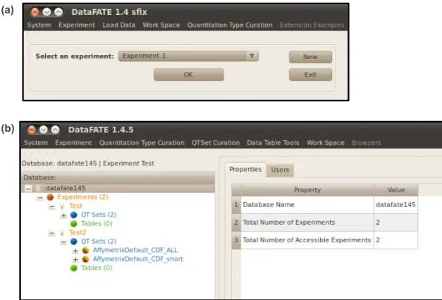
2.3 Previous version of the Data-FATE SIMS (1.4) 47
2.3.1 Implementation 47
2.3.2 Account administration 47
2.3.3 Experiments 47
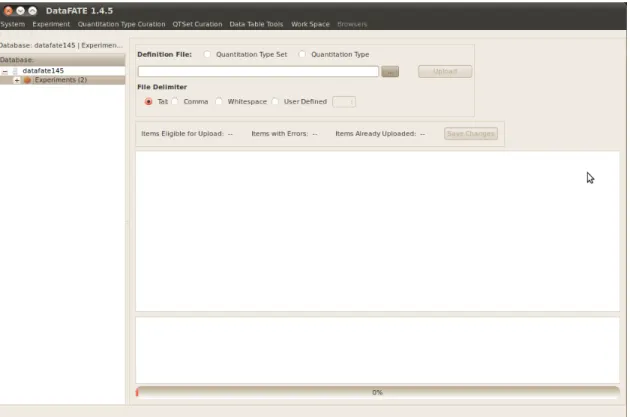
2.3.4 Curating ontological data types 48
2.3.5 Importing and exporting data 49
2.3.6 Querying data 50
2.3.7 Limitations 50
2.4 Current version of the Data-FATE SIMS (1.4.5) 51
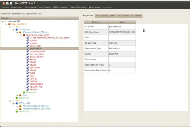
2.4.1 Databases 51
2.4.2 Three-tier architecture 51
2.4.4 Navigation 52
2.4.5 Curating ontological data types 53
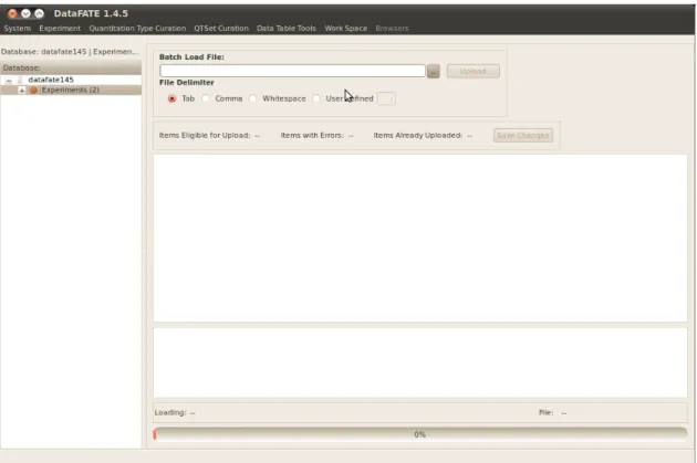
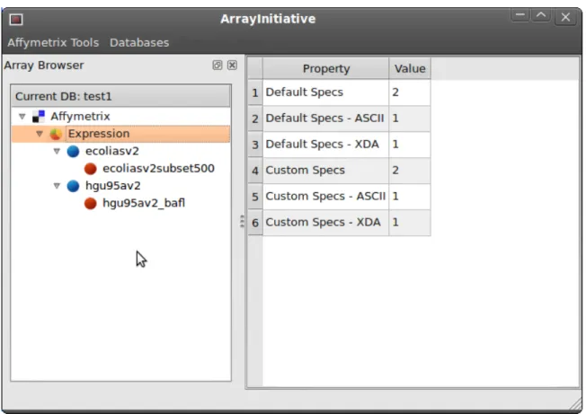
2.4.6 Loading data 56 2.4.7 Tracking workows 56 2.4.8 Testing 57 2.5 Future work 58 CHAPTER 3: ARRAYINITIATIVE 60 3.1 Introduction 60 3.2 Application overview 61 3.2.1 Implementation 63 3.2.2 Functionality 63
3.2.2.1 Context-sensitive (right-click) menus 63 3.2.2.2 Creating and managing multiple databases 63 3.2.2.3 Importing a default array specication 64
3.2.2.4 Importing probe sequences 64
3.2.2.5 Creating a custom array specication le 64 3.2.2.6 Importing a custom array specication 65
3.2.2.7 Exporting an array specication 65
3.2.2.8 Exporting probe sequences for an array specication 65
3.3 Case study 65
3.3.1 The HG-U95Av2 microarray and the Bhattacharjee data set 67
3.3.2 Probe-ltering techniques 67
3.3.2.1 BaFL 67
3.3.2.2 Upton 68
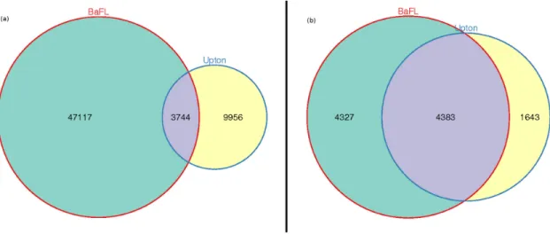
3.3.3 Are the probe-ltering techniques independent? 68
3.3.4 Creating the custom CDFs 70
3.3.6 Dierences in summarized probe set intensities 75
3.3.6.1 MAS 5.0 76
3.3.6.2 dChip 76
3.3.6.3 RMA 78
3.3.7 Case study discussion 78
3.4 Future work 79
CHAPTER 4: PROBESIEVE 81
4.1 Introduction 81
4.2 Methods 84
4.2.1 Hardware and software 84
4.2.2 The E. coli antisense genome array 84
4.2.3 Data sets and databases 84
4.2.4 Re-mapping probes and calculating binding anity 86
4.2.5 Individual factor lters 90
4.2.6 Combining individual lters into lter sets 92
4.2.7 Creating the custom specications 92
4.2.8 Extracting probe intensities and summarizing probe sets 93 4.2.9 Calculating aliated probe correlations 94
4.2.10 Identifying response groups 95
4.2.11 Evaluation and diagnostic methods 97
4.3 Results and discusssion 99
4.3.1 Changes to probe set denitions 99
4.3.2 Binding anity between probes and targets 101
4.3.3 Aliated probe correlations 102
4.3.4 Response groups 105
4.3.5 Response groups vs. aliated probe correlation 108 4.3.6 Dierences in summarized probe set intensities 109
4.3.7 Transcription unit correlation 110 4.3.8 Aliated probe correlation vs. transcription unit correlation 113
4.4 Discussion and future work 114
CHAPTER 5: CONCLUSIONS 117 5.1 Data-FATE 117 5.2 ArrayInitiative 118 5.3 ProbeSieve 119 5.4 Summary 120 REFERENCES 121
LIST OF TABLES
TABLE 3.1: Filter set modications to the HG-95Av2 specication. 73 TABLE 4.1: Hybridization conditions for the OMP simulations. 90
TABLE 4.2: Array specications 93
TABLE 4.3: Probes aected by specic factors. 100
LIST OF FIGURES
FIGURE 1.1: Example of aliated probes 6
FIGURE 1.2: The logical design of an Aymetrix GeneChip 8
FIGURE 1.3: Common mapping problems 27
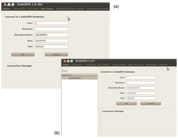
FIGURE 2.1: Comparison of Data-FATE logon screens. 53 FIGURE 2.2: Comparison of Data-FATE post-logon screens and navigation. 54
FIGURE 2.3: Changes to Data-FATE navigation. 55
FIGURE 2.4: Tool for bulk import of ontological data types. 56
FIGURE 2.5: Tool for bulk import of data. 57
FIGURE 3.1: ArrayInitiative main screen 62
FIGURE 3.2: Independent and joint eects of the BaFL and Upton lter sets 69
FIGURE 3.3: Workow for creating the custom CDFs 71
FIGURE 3.4: Number of probe pairs removed by individual lter sets 74 FIGURE 3.5: Dierence between summarized probe set intensities 77
FIGURE 4.1: Changes to probe set denitions 101
FIGURE 4.2: Comparison of aliated probe correlations 103 FIGURE 4.3: Comparison of aliated probe correlations 104 FIGURE 4.4: Prevalence of response groups in each specication 106 FIGURE 4.5: Distribution of correlation within and between response groups 107 FIGURE 4.6: Response groups vs. aliated probe correlation 108 FIGURE 4.7: Dierences in summarized probe set intensities 109 FIGURE 4.8: Correlation for all transcription units 111 FIGURE 4.9: Correlation for all changed transcription units 112 FIGURE 4.10: Aliated probe correlation vs. transcription unit correlation 113
Advances in experimental and computational technology ushered in the current 'omics era, which is characterized by large-scale, high-throughput experiments, and with this wealth of data, it is now possible to start modeling and even building complete biological systems, known respectively as systems biology and synthetic biology. While giving us unprecedented insight into the dynamics of a cell, using the results from omics experiments poses numerous challenges for modern researchers, from storage and organization to scaling modeling environments so they can handle the inputs; the data sets are complex and massive, the associated analysis routines are more involved and the accuracy and precision of the experimental technologies are not suciently examined.
The main focus of our research has been to develop methods and tools to better manage and interpret microarray data. While past research focused most on correctly predicting strong clinical markers of a number of diseases, the ability to understand regulatory networks and underlying mechanisms of the diseases has been a longer range goal. Problems of importance to this research include: How can we improve methods to store and retrieve very large sets of microarray data from a relational database? What physical and technical factors most confound our interpretation of a microarray's measurements? Does deprecating confounded probes allow us to improve the accuracy and precision of microarray measurements? It is essential to address these last two questions before using 'omics data for downstream analyses, such as inferring transciption regulatory networks from microarray data. While microarray data rst raised these questions, they are relevant to 'omics research in general.
1.1 Systems biology, synthetic biology and networks
Systems biology studies multi-component biological systems found in living cells, organisms and communities, seeking to understand how their complex interactions give rise to emergent functions and behaviors at multiple scales, the most fundamen-tal questions and mysteries in biology [1, 2]. Pragmatically, we'd like to use this understanding to identify more robust biomarkers and better predict drug targets, using a systems-level understanding to promote ecacy and limit side eects. More idealistically, our goal is to understand mechanisms that underlie function, including redundancies and fault tolerances. Synthetic biology is the test bed for biological sub-systems, using biotechnology to engineer biosimilar components, including systems not found in nature, creating novel functions and behaviors [3]. For example, the engineering of completely synthetic hydrohexitol nucleic acid polymers (HNAs) and highly modied polymerases carries the promise of creating non-toxic, non-degradable aptamers for binding proteins [4]. Synthetic biology oers the opportunity to build and test systems in isolation from the full complexity of their biological origin. Just as the ndings in systems biology inform the design of synthetic biological systems, the failures and successes in synthetic biology inform our understanding of interactions in natural biological systems [3].
Complex systems can be represented as networks that are modeled as graphs [5]. The rst step is to break down the system into autonomous, or nearly autonomous, subsystems, characterizing the participants, interactions, state parameters, and out-side inputs. Systems biology uses this paradigm of interacting networks to represent many types of cellular systems, including the protein-protein interaction network [6], transcription regulatory network (TRN) [7, 8], signaling network [9, 10] and metabolic network [11, 12]. The network elements are not disconnected, but the specic focus helps identify points where networks modulate one another [13].
char-acterizing its complete structure (static interactome) and modeling which parts are used under specic conditions (dynamic interactome)[14]. The static interactome in-cludes the molecular components (nodes) and all of their possible interactions (edges) - basically, this is an hierarchical parts list [15]. The dynamic interactome describes how the network responds to internal and external signals (e.g. which subnetworks are active, how information propagates through the network, timing etc.). Generally, many data sets are integrated to infer the global structure of the network , while experiments based on time series or individual factors are used to understand the dy-namics [14, 16]. It is also important to understand how the subnetworks interact with each other [17]. Since networks may interact at several points that shift depending on the state, massive amounts of experimental data must be generated across many environmental states and genetic conditions. This data must then be integrated ap-propriately in both spatial and temporal scales [18]. As a data-driven science, it is essential to capture the imperfections of measurement platforms so that integra-tion is performed correctly. The preceding decade of microarray-intensive research has illustrated these problems well, from how sensor design inuences outcomes to the integration challenges presented when read-out devices dier in sensitivity and specicity [19, 20, 21, 22]. The consequences of not removing suspect data are well-documented for clinical tests, but are less publicized with respect to networks [23, 24]. Most genomics experiments that aim to elucidate the dynamics of a system actu-ally capture a series of static snapshots, with the aim of nding the common signature for a particular class of molecule over many cells, although there are also eorts to observe single cells using methods tuned to the time step of the molecular species [25]. As rst expressed by the Functional Genomics Data (FGED) Society (formerly, the Microarray Gene Expression Databases [MGED] Society) in their MIAME standard [26], and later mimicked by many others [27, 28, 29] the data management system that can organize all of the information required to replicate the experiment is
di-cult to design, especially if a consistent model that yields analytical speed is the goal [30, 31]. A signicant result of these early eorts was recognition that controlled, structured vocabularies, or ontologies, must be developed in parallel with the data management hardware and software before eective data integration or data mining could be achieved [32]. Not only are these resources needed for each type of network, but as we move towards integrating networks, additional systems must be developed [33, 34].
For the remainder of this chapter, we'll focus on transcription regulatory networks and the relevant experimental technologies used to characterize them.
1.2 E. coli and its TRN
Transcription regulatory networks are the foundation for all other biological net-works, since proteins originate as transcripts and metabolites are created or moved around by proteins, while together proteins and metabolites modulate transcription; the modulation of transcript production is the initial regulatory network of cells. The most completely studied TRN is that of E. coli, and E. coli is the most completely understood biological system. This is true for many historical and practical reasons: studying prokaryotes is easier than studying eukaryotes since they lack alternative splicing, they have fewer genes and are amenable to genetic manipulation, and many are relatively easy to culture in the lab (especially E. coli). Since E. coli has been a model genetic and experimental organism for many years, and is used extensively in biotechnology, there is an enormous amount of 'omics data. In particular, many of the transcription factors and the units they regulate have been comprehensively characterized across many environmental states and genetic states. A large number of these datasets are in the public domain, and thus serve as a foundation for studies such as ours [35].
1.3 Characterizing TRNs with microarray data
To fully characterize the structure and dynamics of a TRN, you must monitor all of its nodes simultaneously, over many conditions and time points. The rst `omics platform to deliver this capability was the DNA microarray.
DNA microarrays
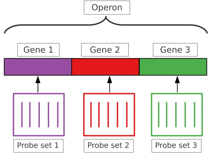
The DNA microarray simultaneously assays all of the complementary nucleic acids in a target solution. Thus it is a popular experimental tool for carrying out many types of genomic and transcriptomic experiments, including gene expression proling, detection of protein-DNA interactions, sequencing, comparative genomics, detection of single-nucleotide polymorphisms (SNPs) and copy number variation (CNV) and detection of alternative splicing. The arrays are constructed as two-dimensional grids of oligonucleotides ('probes'), each unique sequence is covalently axed to a solid support at a specic location ('feature') via spotting or direct synthesis to reactive groups. Genomic features that we wish to assay may vary from a single nucleotide polymorphism (SNP) to units that are tens of thousands of nucleotides in length. Except for SNPs, for most features the probes are shorter than the corresponding targets. This presents an opportunity to sample the target multiple times, and some platforms are designed to accomplish that goal [36]. It is also possible to construct a sampling hierarchy based on co-location of elements on a molecule. As an example, in prokaryotes the genes on an operon may be co-transcribed. So there may be two probes that sample one gene, three probes that sample another, and the 5 probes together sample the operon. To dene this sort of relationship, we use the term 'aliated probes' in this dissertation, meaning any set of probes that measures the same contiguous nucleic acid target. An example of this is shown in Fig. 1.1.
Important distinctions between microarray platforms include the probe length and probe density on the array. Length allows greater sensitivity, but at the expense of specicity unless hybridization conditions can be tuned. The length of probes on
Probe set 1
Probe set 2
Probe set 3
Gene 1
Gene 2
Gene 3
Operon
the most widely used platform is 25nt (Aymetrix, [37]) and on currently marketed commerical platforms the maximum length is 70nt (Agilent, [38]). The 'probe density' can mean either the number of spots per array, which corresponds to the level of genome feature coverage, or to the concentration of the probe within a spot, which correlates to the percent of target that can be bound [39].
Although microarry platform designs dier, the basic procedure for running a microarray experiment is the same for all of them. When a solution of some labeled, puried cellular fraction is assayed against a microarray, a target will hybridize to any suciently complementary probes (intended or not); those not bound after the required reaction time are washed away. Target is labeled if this was not already done, and then the array is scanned, inducing the target-bound uorophore to emit photons (signal), which are then captured and saved as an image le. For the computational scientist, the intensity of the pixels in this le is the starting point for estimating the concentration of each target molecule [39].
Aymetrix DNA microarrays
Aymetrix [37] produces the most widely used of the high-density DNA microar-rays (called the GeneChip®platform). Their complexity results from the promiscu-ous placement of probes with respect to target elements and the multiplicity of probes per biological target. In this case, high probe density means both that there are hun-dreds of thousands to millions of simultaneous measurements to be considered and that the local concentration of probe is very high. The probes are synthesized in-situ, with relatively short lengths (25-33nt). Although the physical design of the arrays a two-dimensional grid of probes is identical to other types of DNA microarrays, the logical design diers signicantly since multiple distinct probes (from 4 to 16 or more, depending on the specic array type) must be merged to report on any given feature. The advantage to such a design is the redundancy of the measurements: probe or tar-get characteristics that fail to report accurately can be removed or reassigned while
leaving sucient probes to faithfully report on the intended target.
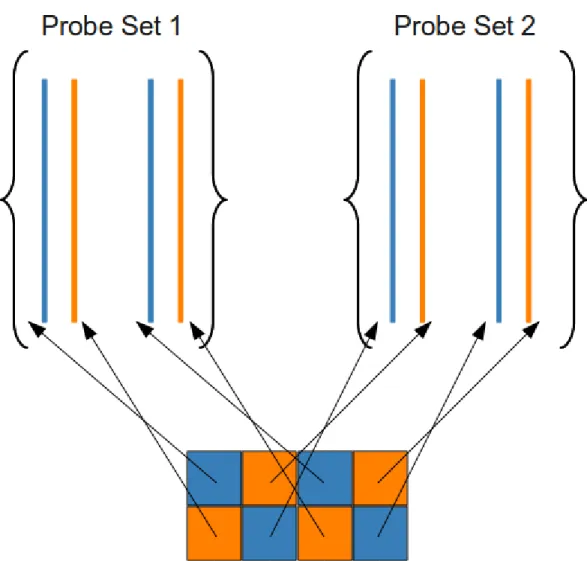
These probes are grouped into sets, as shown in Fig. 1.2, which shows the logical design for 3' IVT expression arrays.
Figure 1.2: The logical design of an Aymetrix GeneChip®.
An Aymetrix-dened probe set is one level in the aliated probe hierarchy which might discriminate variants of a transcript, exon, or SNP. The class of expression arrays is most relevant to our interest in studying TRNs. For several generations of the 3' IVT expression arrays, the basic measurement 'unit' was a probe pair, which included one perfect match (PM) probe and one mismatch (MM) probe, having a
single homomeric transversion at the central position relative to the PM [37]. For example, the E. coli antisense genome array, which will be the focus of Chapter 4 (ProbeSieve), consists of 141,629 probe pairs organized into 7,312 probe sets - 4,426 of them are designed for open reading frames (ORFs), while the remaining 2,886 target intergenic regions of the E. coli K12 genome. Most the of the probe sets have either 15 or 16 probe pairs.
Goals of a microarray experiment
Gene expression microarray experiments are performed to compare the transcrip-tomes produced by dierent biological conditions (e.g. healthy vs. diseased state) and to characterize the structure and dynamics of TRNs across time intervals, conditions and genetic backgrounds. A transcriptome is generally considered to be a description of the genes transcribed above a background level, but in the case of a prokaryote like E. coli, the transcriptome could be considered a description of the transcription units (TUs) produced above a background level, a distinction with a dierence for multi-gene operons. Since regulation aects operons, an accurate inference of the TU level is our goal when describing TRNs.
To infer co-regulation of operons requires that the results of many experiments be compared, since two TUs may well both change without a common regulatory cause .Only if TUs consistently change levels, in the same direction and over many conditions, is it likely that co-regulation is occurring. Microarrays are valuable tools for characterizing the structure and dynamics of TRNs, as researchers can collect a large amount of experimental data across many environmental states and genetic conditions[40, 41].
1.4 Relevance of microarray data to E. coli TRN research
Although high-throughput sequencing (HTS) technologies [42] are starting to sup-plant microarrays as the predominant data-gathering platform for transcript levels, data from DNA microarrays will continue to be produced and used for the
foresee-able future [43]. In part this is because, as an established platform there are core labs producing high quality data and experimentalists well trained in producing the sam-ples. With respect to analysis, the pipelines for data cleansing and data mining are far more mature for microarray data than for RNA-Seq data, and more experts have been trained to use them. Many E coli expression microarray data set are available in public repositories, which is not yet true for HTS data. In fact, NCBI, the manager of the Gene Expression Omnibus microarray data repository [44], has announced that it won't store HTS data because it's too resource-intensive. Because of its size and current lack of model standards, data sharing is more dicult with HTS data than for microarray data. Thus, expression microarray data remain a valuable resource for the discovery of TRNs.
1.5 Microarray data: storage, quality assessment, and integration
Despite 15 years of concentrated eort by a large group of experts, there re-main many challenges associated with storing, managing and using large amounts of microarray data, particularly with respect to determining data quality. This is highlighted by a recent report in which data mining results based on microarray data were shown to be independent of the experimental variables [45].
In section 1.6, we discuss the essential components for storing, managing and using any type of experimental data, which includes building ontologies, developing databases and creating analytical workows. This is the background for research described in Chapter 2 (Data-FATE). Once raw data has been properly organized it can be ltered to identify responses that arise due to the experimental variables and nothing else. There are well-known reproducibility problems associated with microarray data (section 1.7) and known contributing factors (section 1.8). Most analytical workows require an array specication in order to process the ltered (cleansed) data. The review of current methods (sections 1.9 and 1.10) provides the context for Chapters 3 (ArrayInitiative) and 4 (ProbeSieve), which describe a tool for
re-dening probe sets and methods for determining groups of probes with correlated responses to be assigned to such groups.
1.6 Organizing 'omics data
The principle challenges when sharing any type of experimental data include nd-ing mechanisms to communicate the meannd-ing of the data and tools for disseminatnd-ing the data so that it can be retrieved in useful parts as well as entire sets. Data models, database management systems, common vocabularies and shared workows are all essential before a community can make use of a common resource. Although many innovative models and management software environments continue to be developed [46], the maturity of the relational data model and associated management software has led to their preeminence across the spectrum of biological databases [47]. Mean-ingful descriptions require a shared vocabulary. Logically structuring those vocabu-laries allows one to reason about relationships, as biologists demonstrated with the taxonomic tree of life. Thus ontologies have become an important organizing method for biological data. The development and testing of such ontologies has become a re-search focus in its own right, and includes the denition of entities, relationships, data models (e.g. database, exchange formats, etc) and data formats. Finally, to analyze your data consistently (read: arrive at reproducible results), you need to develop and use analytical workows, with varying degrees of rigor.
With the dramatic increase in the volume and complexity of 'omics data (microar-ray, proteomics, next-gen sequencing), the scope of these challenges has increased abruptly. Here we'll discuss each of these challenges ontologies, databases and ana-lytical workows in general, and as they pertain to Aymetrix microarrays speci-cally. This section contains the relevant background for Chapter 2 - Data-FATE. 1.6.1 Ontologies
Humans constantly construct models of the universe around them, whether it be a process model or a data model. Process models describe a set of linked
transforma-tions that allow us to understand how something works and predict the outcome of new inputs or parameters e.g. creating a dynamical model of a transcription regula-tory network [48, 49]. Data models (including ontologies) dene the elements under scrutiny and all of the possible relationships that a process might use to link them. Not only is the data structured, but if the structure is a logical one then consistent representation of the data is assured. This is essential for the discovery of new rela-tionships, which have often emerged when microarray data are used to characterize networks like TRNs [48]. Ontologies are also essential for data integration, which is one of the major challenges in Bioinformatics and systems biology [50, 18].
Denition of an ontology
An ontology as dened in the information sciences is a formal denition of concepts from a particular domain, and the relationship between those concepts. It is essentially a structure, or model, imposed on data in order to make sense of it, and to reason about it. Like the natural scientists' mathematical models, the ontology describes the participants in a physical process, and how those participants interact with each other.
More rigorously, a formal ontology consists of concepts, attributes and relations [51]. A concept is an object, such as a gene, that has at least one attribute (feature), such as genomic location. Concepts and their attributes are analagous to objects and their properties as dened in object-oriented programming. Concepts can range from general to specic and one concept can be a sub-concept of another (with the requirement that they share at least one attribute). Most biological ontologies have used the container (`is-a' and `part-of') relationships only, although more active verbs are slowly being adopted by the Gene Ontology and the Systems Biology Ontolo-gies [52]. For example, you could have a gene concept, with two subconcepts being prokyarotic gene and eukaryotic gene. Finally, an ontology denes relations between concepts; these are like the verbs and connectives in a sentence. For example, a gene
is `expressed' as a gene product, either RNA or protein. In this case this relation is uni-directional, from gene to gene product, indicating a logical limit on the process that transforms one to the other. The easiest way to visualize an ontology is as a graph, where the nodes are concepts and the edges represents a relation between two concepts.
There are two types of ontologies: prescriptive and descriptive. While they both dene concepts, attributes and relations, they dier in how they are constructed and used.
Prescriptive and descriptive ontologies
A prescriptive ontology (shared ontology, top-down ontology, inductive ontology) is one developed, and agreed upon, by the community of use (e.g. microarray re-searchers). This is a top-down approach where the concepts, attributes and rela-tionships are prescribed by a group of experts - it's expected that all new data will conform to the structure of the ontology and that all researchers will use it without modication. While strict and rigid, they're essential for clear communication in the sciences. Having a specialized language for communicating in a particular domain ensures that domain experts are talking about the same things in the same way, with concepts and relationships that are precise and unambiguous . For example, most biologists will agree on the general denition of a gene, even if some attributes vary by sub-specialty. Placed within a formalized, logical structure, prescriptive ontolo-gies also allow reasoning. If you're working within a well-established physical system or experimental procedure where there's deep understanding about the processes and data then a prescriptive ontology likely already exists or is straightforward to develop. Examples of prescriptive ontologies in Bioinformatics include the MGED ontology [26], Gene Ontology (GO) [53], the Systems Biology Ontology (SBO) [54], with its related Kinetic Simulation Algorithm Ontology (KiSAO), and Terminology for the Description of Dynamics (TEDDY)) [54].
Although prescriptive ontologies provide signicant benets, they also have sig-nicant overhead: since they are driven by community consensus, they are slow to update to new concepts and relationships, and as they become both large and complex it can be more dicult to test additions thoroughly. Especially in areas undergoing rapid expansion it is unlikely that everyone agrees on the meaning of the new data. As the ontology grows (or becomes bloated, depending on your perspective), researchers are often forced to use irrelevant terms, and overhead many refuse to accept. Some ontologies have been built with this in mind, with structure that allows pruning, so one retains only the most useful set of terms [55].
A descriptive ontology (bottom-up, inductive) is one built directly from what is known about the data: it describes the experimental factors that aect the data. If you're working in a frontier science, where the understanding of system components and relationships is dynamic, a prescriptive ontology is at best going to be under development. Descriptive ontologies are more limited in scope, being tuned to the task at hand, but allow rapid prototyping of ontologies to support novel applications. Researchers will initially produce multiple competing ontologies but in doing so will test their eectiveness.
Implementing an ontology
Scientists constantly create ontologies, but in the past they have rarely formalized them. It is really the advent of information sharing, and need for data integration from locations across the world, that has driven the growth in scientic ontologies. Data structures required by analytical tools are ontologies, including entity relationship diagrams or an object model used for databases. A structure may be implemented in many ways, depending on the applications that need to access it, such as a relational database schema or XML denition le (DTD, XSD etc.). Data exchanged formats are increasingly using XML. Each implementation will have its own instances e.g. an XML document using a particular schema. Even if you forego the explicit creation
of an ontology, often it's implicit in the implementations or instance data. Some implementations of Bioinformatics ontologies include MAGE-ML [26], GelML [27] and the XML represetation of the Systems Biology Ontology[54].
1.6.2 Databases
While omics experiments generate the high volume of data needed to characterize the structure and dynamics of biological networks, at the end of the experiment you are confronted with a large amount of raw data and a large amount of meta-data to manage. A single microarray (sample) will produce an intensity le with a size ranging from tens to hundreds of megabytes and thousands to millions of measurements; this problem is exacerbated with the newer technologies, where a single HTS run (lane) may produce les in the gigabyte range. This must be multiplied by the number of replicates, samples and conditions, resulting in total data size that is 10 - 100 times larger. The corresponding metadata (experimental and biological information describing the data), and the relationships can be extremely complex. The object model for the Minimal Information about A Microarray Experiment (MIAME, the MAGE-OM) contains 169 objects with very complicated relationships [56].
Relational databases have been the de facto standard for storing large amounts of data for two decades, and in the following sections, we'll discuss them and their limitations. Next, we'll briey discuss NoSql (not-only SQL, non-relational and dis-tributed databases), which have been gaining more prominence as the limits of rela-tional databases have been pushed (and often exceeded) by the recent data explosion in both the sciences and the commercial sector. While NoSql databases are not the focus of this dissertation, the limitations they're meant to work around, and their general approach, apply to the Data-FATE system that we've developed, which is the subject of the research described in Chapter 2.
Relational databases
Relational databases have mature data management software support, and are used by nearly anyone needing to store and retrieve large amounts of data (e.g. cor-porations, researchers etc.). All relational databases adhere to the relational model (to varying degrees), which was developed by E.F. Codd (IBM) in 1970 [57]. The relational model itself is relatively simple to understand, but this simplicity comes with a cost: the software implementation that enforces the relational model is ex-tremely complex and resource intensive. The data structures are manipulated and queried using the Structured Query Language (SQL), a standard honored at some level by all relational database management systems (RDBMSs). Although the lan-guage is relatively simple to learn and use, the actual algorithms for manipulating the relational data structures and retrieving the data sets are quite complex, and performance tuning is an art, not a science.
The relational data model
The relational data model imposes a particular type of logical view on the data structures, carrying with it an ontology. A particular instance of a relational model such as one to model the operon structure of prokaryotic genes is an implementation (realization) of an ontology, whose structure conforms to the rules of the relational model.
The relational model supports three types of general relationships between tables (objects): one-to-one, one-to-many and many-to-many. With enough creativity, one can use a combination of these relationships and metadata tables to create a wide variety of ontological relationships hierarchical, part-of, is-a etc. but the implementation can be tricky since context, semantics and meaning of the non-set relationaships are not inherent to the relational model. In fact, the available op-erators are quite limited and business rules must be used to enforce other types of relationships.
Relational databases for 'omics data
In addition to ontology development, bioinformaticians have spent the past decade developing core data models that provide a common structure to biological informa-tion, the Generic Model Organism Database (GMOD) being one such example [58]. The GMOD is based on the relational model, is extensible in dened ways that allow customization for unique aspects of an organisms biology, and has associated with it tools for populating , querying, visualizing and publishing the database instance [59, 60, 61].
Limitations of relational databases
Relational models do not encompass semantics, terms that shade interpretation by context and process. In addition they do not scale well in their standard conguration, a limitation that genomics labs are now hitting. There are parallel congurations [62, 63] used in the business world, but no freely available systems.
Semantics
The relational model cannot represent parallel valid relations between entities that are distinguished by a temporal function. They also handle many-to-many relation-ships by attening them, using additional entities to bridge these relations. This means there can be many valid ways to faithfully represent ontological objects, at-tributes and relationships, leading to more proliferation of methods, and barriers to integration. There are also limits to computational clarity: columns have only a spe-cic data type, but lack the ability to carry a semantic tag such as units, a feature of any quantitative measurement from a device.
Processing
Relational databases are limited by the hardware on which they reside. By design, these databases are meant to run on a single computer (server) and will have problems when one or all of the machine's resource thresholds are reached: disk space, disk I/O
speed, memory and processing power (CPUs). Even with a multi-terabyte RAID, a machine's disk space is quickly exeeded when storing large numbers of microarrays. Since relational databases retrieve information that is stored on disk, the disk I/O speed is also a major factor for improving the performance of queries. When running many types of queries, relational databases perform their operations in memory, which can quickly be exceeded by large 'omics data sets. Also, most servers have a hard limit on the number of processors that they can have, so even if you can convert your analysis routines to use many processors in parallel, you have a nite amount at your disposal. Finally, the standard way to store data of the same type is to load it all in a single table. This becomes problematic for large 'omics data sets, whether it be microarray data or HTS data, because of the indexing performed by the system to produce data addresses. To run SQL queries eciently, you must therefore dene secondary indices to speed them up. Creating indices takes a signicant amount of time for large tables and the indices themselves require a signicant amount of disk space. If creating an index were a one-time operation, this might be acceptable. However, when you generate more data and want to add it to your database, you will need to drop all of the indices, load the data and then re-create the indices. You can address some of these problems by scaling the server vertically improving the hardware for the machine but there is always a threshold for any single machine. You can also replicate your database in a so-called master/slave setup, but this only helps with handling large access loads, not the size of the database itself.
Given these limitations, developers have come up with some ingenious solutions. In some of them, developers still use relational databases, while in others, they move away from the relational model. In all of them, however, they use the same general guiding principle: partitioning the data (divide-and-conquer).
Sharding and NoSQL strategies
Sharding is the logical partitioning of rows of data, based on some shared char-acteristic (e.g. probe intensities from the same array), and storing them in separate tables, either on the same server or on dierent servers.
If you are constrained to one database server, you face hard limitations on disk space, memory and processing power. If you have multiple machines, you can al-leviate many of these constraints because each server has its own database schema and operates independently from the others (a shared-nothing architecture). Most relational databases don't have any native support for automatic data partitioning or load balancing, so you need to write your own custom solutions.
Although custom software has been developed and marketed to ease the sharding problem, the products tend to be expensive and require signicant maintenance. The diculties and cost inherent in sharding have led many software rms to abandon relational databases and either develop, or use, non-relational solutions.
Non-relational databases don't adhere to the relational model and are usually called NoSQL (not only SQL) databases. We will use the more inclusive term non-relational database management systems (NRDBMS) to refer to them. . Distributed non-relational databases were specically designed to solve the big-data problem: partitioning data across multiple machines and eciently retrieving it. Data is re-trieved through an application-specic API (using parallel processing), rather than a single, standard language such as SQL. Most of these systems do not index data as with relational databases, although some support it. Regardless, these systems store and retrieve data extremely fast. One major drawback of these systems is that they have varying degrees of consistency, as described by the CAP theorem [64]. Notable examples of non-relational databases are Bigtable [65], HBase [66, 67] and Cassandra [68, 69].
1.6.3 Workows
Dening good data models (ontologies) and eectively storing, managing and re-trieving omics data are critical concerns in data-heavy sciences, but these are only preliminary steps to the end goal of research: processing, integrating and analyz-ing the experimental data to characterize the system under study. Bioinformatics is overrun with analysis scripts, pipelines and data formats. Most computational ex-periments consist of many sequential analysis steps, each expecting dierent types of input data and producing dierent types of output data. To join each step, a glue (transformation) module (script) is required to transform the output format of one step into the format expected as input by the next step. This series of steps, tied together, is an analytical workow; analagous to an experimental protocol in the wet lab. In Bioinformatics, these workows quickly become large and complex, and, unlike their lab counterparts, are often poorly documented [70]. Managing these workows becomes cumbersome quickly, reqiring the development of workow man-agement tools.
There are two major aims when developing tools to manage analytical workows: tracking data provenance/data lineage and task automation. Data provenance refers to the documentation of your analysis - what exactly was done at each step. This is critical for science because all experiments including computational experiments must be reproducible. We also want to automate and abstract the workow as much as possible. Analysis and data transformation steps can be viewed as independent modules that we can put together in multiple ways, depending on the experimental goals. We want to dene each step in the workow, connect them and hit run, without the need to oversee and initiate each step.
Workow management systems aim to minimize human interaction during analysis and to make that analysis reproducible, which requires standardized analysis modules, data transformation modules and interfaces between them. These systems represent
a workow as a graph, where a node is a specic analytical task and a directed edge between two nodes typically represents the ow of data from one node to another (i.e. the output of one node is the input of the other, via a specied communication channel and envelope). The systems then manage information about the server where a tool is located, and access and retrieval protocols. The most well-known and widely used Bioinformatics workow management systems are Galaxy [71] and Taverna [72]. These systems suer from one major limitation: the data interfaces input and output for an analytical task are not explicitly dened as an ontological type. Al-though many of the analysis modules support certain data exchange formats as input and output, they don't explicitly state what ontological type is expected or produced. Put another way, they're not semantically `aware' of the data. Their purpose is really to automate processes over distributed services. Since an ontological type can be implemented in many equivalent ways, such as a database table, a delimited text le or a XML le, it would be easier to glue together modules if you knew the data types expected for input and produced as output. For example, a module might expect a 'gene expression' data type as input, which can be instantiated in various ways, and produces a list of dierentially expression as output, which also can be instantiated in many ways.
1.6.4 Summary
The principle challenges when sharing any type of experimental data include nd-ing mechanisms to communicate the meannd-ing of the data and tools for disseminatnd-ing the data so that it can be retrieved in useful parts as well as entire sets. Data models, database management systems, common vocabularies and shared workows are all essential before a community can make use of a common resource.
An ontology allows us to more easily understand and organize data, allows for a consistent representation of data and gives domain experts a controlled vocabulary with which to communicate and standardize analyses. Ontologies are also essential for
communication, automated reasoning, and for integration of disparate data sources. Although having a prescriptive ontology is ideal, it needs wide community buy-in, a deeper understanding of a wide range of relations and stability. In an emerging domain, the interaction problems exists: representing knowledge for the purpose of solving some problem is strongly aected by the nature of the problem and the infer-ence strategy to be applied to the problem [73]. In many cases, a descriptive ontology simply happens, with or without the understanding that the relations are as impor-tant as the vocabulary denitions, because they still have many of the same benets of a prescriptive ontology, excepting community buy-in and completeness. Although there will be multiple competing descriptive ontologies initially, the domain still ben-ets from having them, and they'll most likely be merged into a prescriptive ontology as the domain matures. Besides Data-FATE, which we've developed and will discuss later, we haven't identied any tools for building descriptive ontologies.
Databases allow you to more easily store, manage and retrieve data, as compared to simple le manipulation. Relational databases have been the de facto standard for years for any data intensive eld, including Bioinformatics. However, the dramatic increase in 'omics data (and data in other domains) is straining single-server relational databases, causing many people to develop alternative approaches that use some type of data partitioning (sharding). Some have moved away from the relational model (so-called NoSQL databases), while others integrate partitioning methods on top of existing relational databases. In either case, none of the existing databases integrate ontologies into their systems.
To reproduce the results of a computational experiment, you need to document each process (data transformation, analysis script etc.) in the workow - much like developing a protocol and keeping a lab notebook in the lab. Because there are numerous step to a computational experiments, and even more implementations of a particular type of analysis, workow management systems have been developed to
keep track of and automate analysis pipelines. Several workow management systems have been developed for Bioinformatics, and are a step in the right direction. However, none of them explicitly incorporate ontologies into the input and output interfaces between modules Doing so would make it easier to link separate modules into a single workow.
In Chapter 2 (Data-FATE) we'll discuss how we've integrated ontologies, data partitioning and workows into a single system.
1.7 Accuracy and reproducibility problems with microarray data
*** UNDER CONSTRUCTION ***
The expectations for microrrays were extremely high when the technology rst appeared, especially for applying them to nd multi-genic signatures for diseases (biomarkers). The hope was that physicians could use these signatures to screen for or diagnose a disease in very early stages, since it's always better to identify a disease before its symptoms appear. Requirements for screening are less stringent than for diagnosis, because any ndings will be veried by an independent diagnostic tool, such as qPCR. However, researchers and doctors ultimately hoped to use microarrays for diagnosis, especially for complex diseases with many genes involved. If the molecular signature includes hundreds of genes, PCR validation is not feasible. To be used as a diagnostic tool, the FDA requires that a platform's coverage, accuracy, sensitivity, specicity, reproducibility be rigorously assessed and meet very high standards [74]. Although not an explicit requirement, this is imperative for systems biology research too. To understand complete regulatory networks we need to use a high-throughput, multi-locus experimental technology for studying systems (single-locus technologies are not feasible), but and missing and misleading data has a signicant impact on characterizations of these networks [75] .
The requirements for interpreting microarray data essentially condense to four questions: How much of the target space does the experimental platform actually
measure? Does each probe measure the correct target? Does each probe measure a single target? How well correlated is the probe response with the target amount (i.e. how good is the binding anity between the probe and target)? As discussed in an excellent review by Draghici [74], microarrays had problems with sensitivity, specicity, accuracy, and cross-platform reproducibility, and thus, did not live up to their early promise. This is largely because the technology was very complicated and changed so rapidly that researchers did not suciently examine these questions. Given these known reproducibility problems, what are the factors that cause them? 1.8 Factors aecting the response of microarray probes
Several factors inuence the response of microarray probes, with some of them corresponding to meaningful biological variation while others are sources of unwanted variation. Although there is some overlap, the can break down these factors into four categories: experimental, biological, physical and technical. Of the four, only experimental factors are interesting parts of the experiment (signal) - the rest is noise. 1.8.1 Experimental and biological factors
Experimental factors are the variables that you control during a microarray exper-iment, that, when varied, produce the meaningful phenotypic changes in the biological system under study i.e. experimental factors are the sources of meaningful (desired) measurement variation. For example, the experimental factors could be disease state and the goal of the study might be to determine the dierence in the transcriptomes of healthy and diseased tissues. Biological factors correspond to natural variation be-tween individuals, such as dierences in a genotypic population or dierences bebe-tween the same cells caused by stochastic processes. These factors are usually sources of unwanted variation, but can sometimes be controlled e.g. by using inbred lines in your experiment.
1.8.2 Physical and technical factors
Physical and technical factors (and composites of them) introduce unwanted vari-ation into microarray measurements that have nothing to do with the experiment or biology of the system, but that still aect a probe's sensitivity, specicity, accuracy and precision. Physical factors directly aect the binding anity between the probe and target, causing a bias in the amount of probe-target duplexes that can form, and in turn, biasing the scanned probe intensities; these factors correspond to the ther-modynamic and biochemical characteristics of a probe and target. Technical factors correspond to variation introduced by microarray design, manufacturing, platform dierences and experimental handling of sample material. Composite factors are a combination of one or more physical or technical factors. Here we'll discuss the fac-tors relevant to this study: probe and target secondary structure, probe-to-target mapping, probe sequence motifs and sensitivity range of the scanner.
Probe and target secondary structure
Secondary structure - present in the probe, target or both - is a physical factor, directly aecting the binding anity between the probe and its target. Although probe and target monomer structures sometimes increase the binding anity (duplex stabilization), most often they have no eect or diminish the duplex stability. If the binding anity between a probe and target is zero, the probe will indicate that the target is not present (false positive); if the binding anity is non-zero but not perfect, the probe will underreport the amount of target present (negative bias).
This becomes complicated because a probe's sequence need not exactly match (be perfectly complementary to) the target's sequence to bind strongly [76, 77]. For example, the Kane criteria only requires a minimum nucleation of 15 nucleotides and 75% sequence identity between probe and target for hybridization [78]. Conversely, even if a probe sequence is an exact match to a target sequence, it's possible, due to thermodynamic and kinetic eects, that the binding anity between them is zero.
For example, a probe or target might have internal secondary structure (monomer) that is more favorable than the duplex, a target homodimer and heterodimer might be more favorable than the duplex or the duplex might be kinetically unfavorable (although thermodynamically favorable).
If the concentration of probe and target were nearly equal, this would be a moot issue because a probe-target pair with an exact alignment will nearly always outcom-pete an inexact alignment. However, the probe concentration on all array types is signicantly higher than the target's, in order to drive the monomer reactants to the duplex product. This allows less optimal, inexact alignments to bind to the same probe as well, without much competition.
Probe-to-target mapping
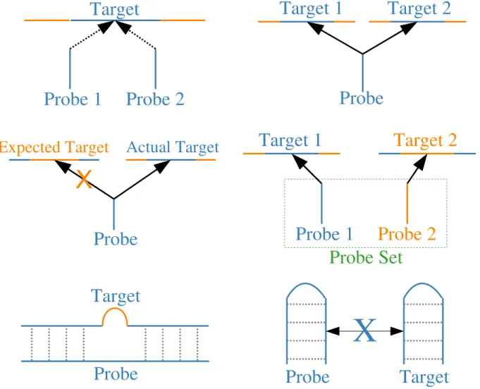
Probe-to-target mapping problems are composite factors that confound our inter-pretation of a probe measurement by making us think that a measurement reects one target (the intended target), when it actually measures a dierent target or the intended target and a dierent target - this causes false positives and negatives. The most common mapping problems are cross-hybridization (to additional and un-intended targets) and missing targets, as shown in Fig. 1.3. If a probe measures multiple targets, it's said to cross-hybridize, which typically causes false positives, false negatives and inated estimates of target concentration; if a probe measures a single target for which it was not designed, it's said to have an unintended target, which results in both false positives and negatives; if a probe can't measure the tar-get for which it was designed, it's said to have a missing tartar-get, which causes false negatives.
Probe-to-target mapping problems can happen for several reasons. Updates to the genome annotation are the most common, and widely understood, technical fac-tor that can cause problems. Since probes especially those on an expression or SNP/CNV array are typically designed against exact alignments to a certain
ver-Probe 1
Probe 2
Target
Actual Target
Expected Target
Probe
X
Probe
Target
Target 1
Target 2
Probe
Target 1
Target 2
Probe 1
Probe 2
Probe Set
X
Probe
Target
sion of a genome annotation, any updates to the annotation will likely change the expected targets for a probe. Probes thought to have a single target with the previous genome annotation might now, with the updated genome annotation, be known to cross-hybridize, have a dierent target than intended or have no target.
High binding anity between probes and targets with inexact alignments is a common, but not widely understood, physical factor that can cause probe-to-target mapping problems. Since none of the major microarray platforms designed their probes using inexact alignments to the genome, they most likely missed a signicant number of potential targets for a probe. This means that a even if a probe has a single, correct target, based upon an exact alignment, it might still cross-hybridize to several other unintended targets to which it is not perfectly complementary. However, inexact alignments can also be an advantage. If we discover that a probe without an exact alignment has an inexact alignment to another target, we can re-purpose it to measure the other target, assuming the binding anity between them is suciently high.
Probe sequence motifs
Probe sequence motifs, like secondary structure, are most likely a physical factor that aects the binding anity between a probe and its target, although the mech-anism is not always known. The two most common types are G-runs and primer spacers [79, 80]. Probes with a G-run motif have at least one instance of ≥4 Gs in a
row, while probes with a primer spacer motif have at least one instance of CCTCC. The latter is incorporation of a T7-binding site when a cDNA is amplied to cRNA during target preparation and is only a problem when the target is prepared in this manner; the problem arises because the probes were not designed against this fea-ture and it causes cross-hybridization in some cases. Both sequence motifs result in probes that report a signicantly greater intensity than the target amount should cause, and their expression proles are more highly correlated with each other across
conditions, than they are with other probes designed to measure the same target (e.g. other members of an Aymetrix probe set). Whatever the mechanism, these probes usually overreport the amount of target present (positive bias).
Sensitivity range of the scanner (linear range)
For Aymetrix scanners, only reported intensities between 200 and 20,000 uo-rescence units are consistent - this is the sensitvity range of the scanner [81, 82]. For genes that aren't expressed, the reported intensity is often below the sensitivity range (< 200), and behaves inconsistently. You can only say that the intensity, at most, was 200. For probes with a reported intensity above the sensitivity range (> 20,000), you can only say that the intensity is at least 20,000. Whether above or below, you must set and enforce limits on your interpretation of your measurement.
1.8.3 Summary
Several physical and technical factors introduce unwanted variation into a probe's measurements, confounding our ability to accurately interpret a microarray exper-iment. As with any measurement platform, the best policy is to identify aected sensors (probes, in this case) and then either x or remove them.
1.9 Correcting for physical and technical factors
Both statistical and factor-based approaches have been developed to identify and adjust for probes whose intensities don't accurately reect relative amount of the intended targets. Statistical approaches were developed rst, followed by factor-based methods. Here we'll the merits and limitations of each approach.
1.9.1 Statistical methods
Statistical approaches, such as RMA, GC-RMA , dChip and MAS5.0 [83, 84, 85, 86], follow a common workow: background correction, standardization, normaliza-tion, identication and removal of outlier probe measurements and, where necessary, summarization (particularly for Aymetrix arrays). There are many benets to the statistical approaches: they're easy to use, good at removing generalized
measure-ment variation following an expected distribution and are already implemeasure-mented and tested in major analysis packages, such as those found in BioConductor [87]. However, they handle the many factors causing variation by merging them into a single `noise' factor. By not treating the factors separately (that is, knowing what is being and removed and why) meaningful experimental and biological measurements are likely to be removed along with the undesired technical and physical factors.
1.9.2 Factor-based methods
In contrast, factor-based approaches identify probes inuenced by specic physical and technical factors and adjust the interpretation of the measurements accordingly. When a probe is aected by a factor, it's typically handled in three ways: it's depre-cated, its relationship to a target is updated, or its reported intensity is adjusted (the second and third can both happen for the same probe). Several benets recommend the factor-based approaches: you're less likely to remove the meaningful biological and experimental variation and the treatment of probes is consistent across all conditions. However, factor-based approaches require a signicant amount of data management and can be computationally challenging, especially when creating usable les to reect changes to the array specication. Despite these challenges, many studies show that, for any experiment, removing known factors that confound measurements improves the reliability and reproducibility of the data analysis.
1.9.3 Single-factor studies
Here we discuss several single-factor studies (relevant to our research) that have been performed on Aymetrix microarrays. We discuss the general approach and how, by accounting for these factors, the interpration of the experiment improved. Probe-to-target mapping
Shortly after Aymetrix released the sequence information for their arrays into the public domain, several researchers analyzed the probe set denitions [88, 89, 90, 91, 92, 93, 80], identifying a number of potential problems with the original denitions that
could produce measurement error within a probe set. They then proposed several bioinformatics methods for re-dening the probe sets to solve these problems (e.g. creating a custom array specication), intending to reduce the measurement error and to make the aggregated measurements more biologically relevant. In many cases, these groups validated their re-denition strategies by showing that their custom probe set denitions, when compared to the Aymetrix default, signicantly changed the dierential expression results. In some cases, subsequent studies showed that the re-denition strategy signicantly improved the correlation between microarray measurements and experimental results. The custom probe set denitions of Dai et al. [89], and two later studies using them [94, 95], illustrate how custom array specications can signicantly improve microarray measurements and the conclusions drawn from them.
For several Aymetrix expression arrays, Dai et al. [89] re-dened the original probe sets into gene-, transcript- and exon-specic probe sets. They used the most up-to-date versions of several public genome databases, such as UniGene [96] and Refseq [96], in this process, and then created custom CDFs for each source. In one case, they used an updated version of UniGene to dene a gene-specic CDF for the Aymetrix HG-U133A chip and then reanalyzed data from a cardiac tissue study (GSE974) [97]; comparing the updated CDF and the original CDF, they found between 30-40% dierences in those genes predicted to be signicantly dierentially expressed between the two. When performing a similar analysis with other custom CDFs, they found between 30-50% dierences in predicted dierential expression. Subsequently, Sandberg et al. [95] showed that Dai's custom probe set denitions, when compared to the original denitions, improved the accuracy and precision of transcript estimates for a set of cross-lab replicate arrays [98]. In particular, their accuracy metrics showed that the microarray measurements became more similar to those measured by RT-PCR. Later, Mieczkowski et al. [94] showed that Dai's
custom CDFs signicantly improved the correlation between microarray expression proles and RT-PCR expression proles. Thus, re-dening array specications can potentially improve the down-stream analysis of Aymetrix microarrays.
Sequence motifs
Upton et al. [79, 80] reported that probes with certain sequence motifs have intensities that are uncorrelated with the other probes in the same probe set; however, they tend to correlate well with any probes having the same sequence motif, regardless of probe set membership. In this case study, we will focus on the two major types of problematic sequence motifs identied by Upton et al. [80]: G-runs and primer spacers. Probes with the G-run motif, ≥4Gs in a row, tend to produce consistently
high intensities, with some position dependence. The primer spacer motif, CCTCC, is related to the incorporation of a T7-binding site when a mRNA is amplied during target preparation. When the target is amplied in this manner, the probe intensities tend to be higher than most, introducing a spurious correlation similar to that seen with G-runs. Since both of these sequence motifs introduce a systematic bias when summarizing probe set intensities, any probes including them should be removed from a CDF prior to calculating expression values. This is always true for the G-run motif and is true for the primer spacer motif when the target is amplied by incorporating a T7-binding site.
1.9.4 Multi-factor studies
While several studies have investigated and corrected for individual physical and technical factors, few studies have integrated them into a consolidated pipeline. Here we discuss two such studies, BaFL and Lo-BaFL. The BaFL pipeline is the basis for the research in Chapter 4.
Biologically-applied lter levels (BaFL)
Thompson et al. [99] developed a white box pipeline Biologically-applied Filter Levels (BaFL) to identify and lter microarray probes that are likely to report
in-correct or misleading intensities based upon certain biological properties, such as the presence of SNPs in the probe sequence (e.g. as identied by AyMapsDetector [100]), probe cross-hybridization, internal structure in either the probe or target sequence that reduces binding anity, and probe intensities that fall outside the sensitivity range of the scanning device [81, 82]. They tested their lter set on two indepen-dent microarray studies of human lung adenocarcinoma and showed that it improved concordance between lists of signicantly dierentially expressed genes and sample classication.
Lo-BaFL
Baciu et al. [ms in review] developed the Lo-BaFL pipeline, which adapts the orignal BaFL pipeline to the Agilent platform and also extends it by accounting for the Upton sequence motifs.
1.9.5 Summary
Factor-based methods identify and correct for probes inuenced by known phys-ical and technphys-ical factors. Although purely statistphys-ical methods are easier and less computationally intensive, factor-based methods are preferred because they're less likely to remove meaningful sources of measurement variation. Many single-factor methods have been developed for dealing with probes aected by incorrect probe-to-target mapping, interfering secondary structure, problematic sequence motifs and scanner limitations. However, by only accounting for a single factor, your interpreta-tion of the experiment, while better, are still suspect. To comprehensively improve an array, you need to account for all factors known to aect probe measurements. Two such multi-factor pipelines have been developed, BaFL and Lo-BaFL (an exten-sion of BaFL to the Agilent platform), and have been shown to dramatically improve experimental interpretations. To date, a version of the BaFL pipeline doesn't exist for the Aymetrix E. coli arrays.